© The Author(s), under exclusive license to APress Media, LLC, part of Springer Nature 2022
D. Kuhn, T. KyteExpert Oracle Database Architecturehttps://doi.org/10.1007/978-1-4842-7499-6_14

14. Parallel Execution

Darl Kuhn1   and Thomas Kyte2
(1)
Morrison, CO, USA
(2)
Denver, CO, USA
 

Parallel execution, a feature of Oracle Enterprise Edition (it is not available in the Standard Edition), is the ability to physically break a large serial task (any DML, or DDL in general) into many smaller bits that may all be processed simultaneously. Parallel executions in Oracle mimic the real-life processes we see all of the time. For example, you would not expect to see a single individual build a house; rather, many people team up to work concurrently to rapidly assemble the house. In that way, certain operations can be divided into smaller tasks and performed concurrently; for instance, the plumbing and electrical wiring can take place concurrently to reduce the total amount of time required for the job as a whole.

Parallel execution in Oracle follows much the same logic. It is often possible for Oracle to divide a certain large job into smaller parts and to perform each part concurrently. In other words, if a full table scan of a large table is required, there is no reason why Oracle cannot have four parallel sessions, P001P004, perform the full scan together, with each session reading a different portion of the table. If the data scanned by P001P004 needs to be sorted, this could be carried out by four more parallel sessions, P005P008, which could ultimately send the results to an overall coordinating session for the query.

Parallel execution is a tool that, when wielded properly, may result in increased orders of magnitude with regard to response time for some operations. When it’s wielded as a “fast = true” switch, the results are typically quite the opposite. In this chapter, the goal is not to explain precisely how parallel query is implemented in Oracle, the myriad combinations of plans that can result from parallel operations, and the like; this material is covered quite well in Oracle Database Administrator’s Guide, Oracle Database Concepts manual, Oracle VLDB and Partitioning Guide, and, in particular, Oracle Database Data Warehousing Guide. This chapter’s goal is to give you an understanding of what class of problems parallel execution is and isn’t appropriate for. Specifically, after looking at when to use parallel execution, we will cover
  • Parallel query: This is the capability of Oracle to perform a single query using many operating system processes or threads. Oracle will find operations it can perform in parallel, such as full table scans or large sorts, and create a query plan that does them in parallel.

  • Parallel DML (PDML): This is very similar in nature to parallel query, but it is used in reference to performing modifications (INSERT, UPDATE, DELETE, and MERGE) using parallel processing. In this chapter, we’ll look at PDML and discuss some of the inherent limitations associated with it.

  • Parallel DDL: Parallel DDL is the ability of Oracle to perform large DDL operations in parallel. For example, an index rebuild, creation of a new index, loading of data via a CREATE TABLE AS SELECT, and reorganization of large tables may all use parallel processing. This, I believe, is the sweet spot for parallelism in the database, so we will focus most of the discussion on this topic.

  • Parallel load: External tables and SQL*Loader have the ability to load data in parallel. This topic is touched on briefly in this chapter and in Chapter 15.

  • Procedural parallelism: This is the ability to run our developed code in parallel. In this chapter, I’ll discuss two approaches to this. The first approach involves Oracle running our developed PL/SQL code in parallel in a fashion transparent to developers (developers are not developing parallel code; rather, Oracle is parallelizing their code for them transparently). The other is something I term “do-it-yourself parallelism,” whereby the developed code is designed to be executed in parallel.

  • Parallel recovery: Another form of parallel execution in Oracle is the ability to perform parallel recovery. Parallel recovery may be performed at the instance level, perhaps by increasing the speed of a recovery that needs to be performed after a software, operating system, or general system failure (e.g., an unexpected power outage). Parallel recovery may also be applied during media recovery (e.g., restoration from backups). It is not my goal to cover recovery-related topics in this book, so I’ll just mention the existence of parallel recovery in passing. For further reading on the topic, see the Oracle Database Backup and Recovery User’s Guide.

Now that you have a brief introduction to parallel execution, let’s get started with when it would be appropriate to use this feature.

When to Use Parallel Execution

Parallel execution can be fantastic. It can allow you to take a process that executes over many hours or days and complete it in minutes. Breaking down a huge problem into small components may, in some cases, dramatically reduce the processing time. However, one underlying concept that is useful to keep in mind while considering parallel execution is summarized by this very short quote from Oracle expert Jonathan Lewis:

PARALLEL QUERY option is essentially nonscalable.

Although this quote is many years old as of this writing, it is as valid today, if not more so, as it was back then. Parallel execution is essentially a nonscalable solution. It was designed to allow an individual user or a particular SQL statement to consume all resources of a database. If you have a feature that allows an individual to make use of everything that is available, and then allow two individuals to use that feature, you’ll have obvious contention issues. As the number of concurrent users on your system begins to overwhelm the number of resources you have (memory, CPU, and I/O), the ability to deploy parallel operations becomes questionable. If you have a four-CPU machine, for example, and you have 32 users on average executing queries simultaneously, the odds are that you do not want to parallelize their operations. If you allowed each user to perform just a “parallel 2” query, you would now have 64 concurrent operations taking place on a machine with just four CPUs. If the machine was not overwhelmed before parallel execution, it almost certainly would be now.

In short, parallel execution can also be a terrible idea. In many cases, the application of parallel processing will only lead to increased resource consumption, as parallel execution attempts to use all available resources. In a system where resources must be shared by many concurrent transactions, such as in an OLTP system, you would likely observe increased response times due to this. It avoids certain execution techniques that it can use efficiently in a serial execution plan and adopts execution paths such as full scans in the hope that by performing many pieces of the larger, bulk operation in parallel, it would be better than the serial plan. Parallel execution, when applied inappropriately, may be the cause of your performance problem, not the solution for it.

So, before applying parallel execution, you need the following two things to be true:
  • You must have a very large task, such as the full scan of 500GB of data.

  • You must have sufficient available resources. Before parallel full scanning 500GB of data, you want to make sure that there is sufficient free CPU to accommodate the parallel processes as well as sufficient I/O. The 500GB should be spread over more than one physical disk to allow for many concurrent read requests to happen simultaneously, there should be sufficient I/O channels from the disk to the computer to retrieve the data from disk in parallel, and so on.

If you have a small task, as generally typified by the queries carried out in an OLTP system, or you have insufficient available resources, again as is typical in an OLTP system where CPU and I/O resources are often already used to their maximum, then parallel execution is not something you’ll want to consider. So you can better understand this concept, I present the following analogy.

A Parallel Processing Analogy

I often use an analogy to describe parallel processing and why you need both a large task and sufficient free resources in the database. It goes like this: suppose you have two tasks to complete. The first is to write a one-page summary of a new product. The other is to write a ten-chapter comprehensive report, with each chapter being very much independent of the others. For example, consider this book: this chapter, “Parallel Execution,” is very much separate and distinct from the chapter titled “Redo and Undo”—they did not have to be written sequentially.

How do you approach each task? Which one do you think would benefit from parallel processing?

One-Page Summary

In this analogy, the one-page summary you have been assigned is not a large task. You would either do it yourself or assign it to a single individual. Why? Because the amount of work required to parallelize this process would exceed the work needed just to write the paper yourself. You would have to sit down, figure out that there should be 12 paragraphs, determine that each paragraph is not dependent on the other paragraphs, hold a team meeting, pick 12 individuals, explain to them the problem and assign them each a paragraph, act as the coordinator and collect all of their paragraphs, sequence them into the right order, verify they are correct, and then print the report. This is all likely to take longer than it would to just write the paper yourself, serially. The overhead of managing a large group of people on a project of this scale will far outweigh any gains to be had from having the 12 paragraphs written in parallel.

The exact same principle applies to parallel execution in the database. If you have a job that takes seconds or less to complete serially, then the introduction of parallel execution and its associated managerial overhead will likely make the entire thing take longer.

Ten-Chapter Report

But consider the second task. If you want that ten-chapter report fast—as fast as possible—the slowest way to accomplish it would be to assign all of the work to a single individual (trust me, I know—look at this book! Some days I wished there were 15 of me working on it). So you would hold the meeting, review the process, assign the work, act as the coordinator, collect the results, bind up the finished report, and deliver it. It would not have been done in one-tenth the time, but perhaps one-eighth or so. Again, I say this with the proviso that you have sufficient free resources. If you have a large staff that is currently not doing anything, then splitting the work up makes complete sense.

However, consider that as the manager, your staff is multitasking and they have a lot on their plates. In that case, you have to be careful with that big project. You need to be sure not to overwhelm them; you don’t want to work them beyond the point of exhaustion. You can’t delegate out more work than your resources (your people) can cope with; otherwise, they’ll quit. If your staff is already fully utilized, adding more work will cause all schedules to slip and all projects to be delayed.

Parallel execution in Oracle is very much the same. If you have a task that takes many minutes, hours, or days, then the introduction of parallel execution may be the thing that makes it run eight times faster. But if you are already seriously low on resources (the overworked team of people), then the introduction of parallel execution would be something to avoid, as the system will become even more bogged down. While the Oracle server processes won’t quit in protest, they could start running out of RAM and failing or just suffer from such long waits for I/O or CPU as to make it appear as if they were doing no work whatsoever.

If you keep this in mind, remembering never to take an analogy to illogical extremes, you’ll have the commonsense guiding rule to see if parallelism can be of some use. If you have a job that takes seconds, it is doubtful that parallel execution can be used to make it go faster—the converse would be more likely. If you are low on resources already (i.e., your resources are fully utilized), adding parallel execution would likely make things worse, not better. Parallel execution is excellent for when you have a really big job and plenty of excess capacity. In this chapter, we’ll take a look at some of the ways we can exploit those resources.

Parallel Query

Parallel query allows a single SQL SELECT statement to be divided into many smaller queries, with each component query being run concurrently, and then the results from each combined to provide the final answer. For example, consider the following query after connecting to my pluggable database:
$ sqlplus eoda/foo@PDB1
SQL> select count(status) from big_table;
Using parallel query, this query could use some number of parallel sessions, break the BIG_TABLE into small, nonoverlapping slices, and then ask each parallel session to read the table and count its section of rows. The parallel query coordinator for this session would then receive each of the aggregated counts from the individual parallel sessions and further aggregate them, returning the final answer to the client application. Graphically, it might look like Figure 14-1.
../images/319655_4_En_14_Chapter/319655_4_En_14_Fig1_HTML.jpg
Figure 14-1

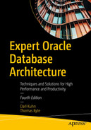
Parallel select count (status) depiction

Note

There is not a one-to-one mapping between processes and files as Figure 14-1 depicts. In fact, all of the data for BIG_TABLE could have been in a single file, processed by four parallel processes. Or, there could have been two files processed by the four, or any number of files in general.

The p000, p001, p002, and p003 processes are known as parallel execution servers, sometimes also referred to as parallel query (PQ ) slaves . Each of these parallel execution servers is a separate session connected as if it were a dedicated server process. Each one is responsible for scanning a nonoverlapping region of BIG_TABLE, aggregating their result subsets, and sending back their output to the coordinating server—the original session’s server process—which will aggregate the subresults into the final answer.

We can see this in an explain plan. Using a BIG_TABLE with ten million rows in it (see the “Setting Up Your Environment” section at the beginning of the book for details on creating a BIG_TABLE), we’ll walk through enabling a parallel query for that table and discover how we can see parallel query in action. This example was performed on a four-CPU machine with default values for all parallel parameters; that is, this is an out-of-the-box installation where only necessary parameters were set, including SGA_TARGET (set to 1GB), DB_BLOCK_SIZE (set to 8KB), and PGA_AGGREGATE_TARGET (set to 512MB). Initially, we would expect to see the following plan:
SQL> explain plan for select count(status) from big_table;
Explained.
SQL> select * from table(dbms_xplan.display(null, null, 'TYPICAL -ROWS -BYTES -COST'));
---------------------------------------------------
|  Id | Operation          | Name      | Time     |
---------------------------------------------------
|   0 | SELECT STATEMENT   |           | 00:00:03 |
|   1 |  SORT AGGREGATE    |           |          |
|   2 |   TABLE ACCESS FULL| BIG_TABLE | 00:00:03 |
---------------------------------------------------
Note

Different releases of Oracle have different default settings for various parallel features—sometimes radically different settings. Do not be surprised if you test some of these examples on older releases and see different output as a result of that.

That is a typical serial plan. No parallelism is involved because we did not request parallel query to be enabled, and by default it will not be. We may enable parallel query in a variety of ways, including the use of a hint directly in the query or by altering the table to enable the consideration of parallel execution paths (which is the option we use here). We can specifically dictate the degree of parallelism to be considered in execution paths against this table. For example, we can tell Oracle, “We would like you to use parallel degree 4 when creating execution plans against this table.” This translates into the following code:
SQL> alter table big_table parallel 4;
Table altered.

I prefer to just tell Oracle, “Please consider parallel execution, but you figure out the appropriate degree of parallelism based on the current system workload and the query itself.” That is, let the degree of parallelism vary over time as the workload on the system increases and decreases. If we have plenty of free resources, the degree of parallelism will go up; in times of limited available resources, the degree of parallelism will go down. Rather than overload the machine with a fixed degree of parallelism, this approach allows Oracle to dynamically increase or decrease the amount of concurrent resources required by the query.

We simply enable parallel query against this table via the ALTER TABLE command :
SQL> alter table big_table parallel;
Table altered.
That is all there is to it—parallel query will now be considered for operations against this table. When we rerun the explain plan, this time we see the following:
SQL> explain plan for select count(status) from big_table;
Explained.
SQL> select * from table(dbms_xplan.display(null, null, 'TYPICAL -ROWS -BYTES -COST'));
---------------------------------------------------------------------------
|  Id | Operation              | Name      | Time     |    TQ  |IN-OUT| PQ Distrib |
---------------------------------------------------------------------------
|   0 | SELECT STATEMENT       |           | 00:00:01 |        |      |            |
|   1 |  SORT AGGREGATE        |           |          |        |      |            |
|   2 |   PX COORDINATOR       |           |          |        |      |            |
|   3 |    PX SEND QC (RANDOM) | :TQ10000  |          |  Q1,00 | P->S | QC (RAND)  |
|   4 |     SORT AGGREGATE     |           |          |  Q1,00 |PCWP |            |
|   5 |      PX BLOCK ITERATOR |           | 00:00:01 |  Q1,00 | PCWC |            |
|   6 |       TABLE ACCESS FULL| BIG_TABLE | 00:00:01 |  Q1,00 | PCWP |            |
---------------------------------------------------------------------------

Notice the aggregate time for the query running in parallel was 00:00:01 as opposed to the previous estimate of 00:00:03 for the serial plan. Remember, these are estimates, not promises!

If you read this plan from the bottom up, starting at ID=6, it shows the steps described in Figure 14-1. The full table scan would be split up into many smaller scans (step 5). Each of those would aggregate their COUNT(STATUS) values (step 4). These subresults would be transmitted to the parallel query coordinator (steps 2 and 3), which would aggregate these results further (step 1) and output the answer.

DEFAULT PARALLEL EXECUTION SERVERS
When an instance starts, Oracle uses the value of the PARALLEL_MIN_SERVERS initialization parameter to determine how many parallel execution servers to automatically start. These processes are used to service parallel execution statements. The minimum value of PARALLEL_MIN_SERVERS is calculated from CPU_COUNT * PARALLEL_THREADS_PER_CPU * 2. In a Linux/UNIX environment, you can view these processes using the ps command:
$ ps -aef | grep '^oracle.*ora_p00._'
oracle    1198     1  0 17:20 ?        00:00:02 ora_p000_CDB
oracle    1200     1  0 17:20 ?        00:00:02 ora_p001_CDB
oracle    1215     1  0 17:20 ?        00:00:00 ora_p002_CDB
oracle    1217     1  0 17:20 ?        00:00:00 ora_p003_CDB
oracle    1569     1  0 17:21 ?        00:00:00 ora_p004_CDB
oracle    1571     1  0 17:21 ?        00:00:00 ora_p005_CDB
If we are curious enough to want to watch parallel query, we can easily do so using two sessions. In the session that we will run the parallel query in, we’ll start by determining our SID:
SQL> select sid from v$mystat where rownum = 1;
       SID
----------
       258
In another session, we get this query ready to run (but don’t run it yet, just type it in!):
SQL> select sid, qcsid, server#, degree from v$px_session where qcsid = 258
Now, going back to the original session that we queried the SID from, we’ll start the parallel query. In the session with the query setup, we can run it now and see output similar to this:
  /
       SID      QCSID    SERVER#     DEGREE
---------- ---------- ---------- ----------
        26        258          1          8
       102        258          2          8
       177        258          3          8
       267        258          4          8
        23        258          5          8
        94        258          6          8
       169        258          7          8
        12        258          8          8
       258        258
9 rows selected.
We see here that our parallel query session (SID=258) is the query coordinator SID (QCSID) for nine rows in this dynamic performance view. Our session is coordinating or controlling these parallel query resources now. We can see each has its own SID; in fact, each is a separate Oracle session and shows up as such in V$SESSION during the execution of our parallel query:
SQL> select sid, username, program from v$session
    where sid in ( select sid
                     from v$px_session
                    where qcsid = 258 );
       SID USERNAME   PROGRAM
---------- --------   ---------------------------
        12 EODA       oracle@orclvm (P007)
        23 EODA       oracle@orclvm (P004)
        26 EODA       oracle@orclvm (P000)
        94 EODA       oracle@orclvm (P001)
       102 EODA       oracle@orclvm (P005)
       169 EODA       oracle@orclvm (P006)
       177 EODA       oracle@orclvm (P002)
       258 EODA       sqlplus@orclvm (TNS V1-V3)
       267 EODA       oracle@orclvm (P003)
9 rows selected.
Note

If a parallel execution is not occurring in your system, do not expect to see the parallel execution servers in V$SESSION. They will be in V$PROCESS, but will not have a session established unless they are being used. The parallel execution servers will be connected to the database, but will not have a session established. See Chapter 5 for details on the difference between a session and a connection.

In a nutshell, that is how parallel query—and, in fact, parallel execution in general—works. It entails a series of parallel execution servers working in tandem to produce subresults that are fed either to other parallel execution servers for further processing or to the coordinator for the parallel query.

In this particular example, as depicted, we had BIG_TABLE spread across four separate devices in a single tablespace (a tablespace with four datafiles). When implementing parallel execution, it is generally optimal to have your data spread over as many physical devices as possible. You can achieve this in a number of ways:
  • Using RAID striping across disks

  • Using ASM, with its built-in striping

  • Using partitioning to physically segregate BIG_TABLE over many disks

  • Using multiple datafiles in a single tablespace, thus allowing Oracle to allocate extents for the BIG_TABLE segment in many files

In general, parallel execution works best when given access to as many resources (CPU, memory, and I/O) as possible. However, that is not to say that nothing can be gained from parallel query if the entire set of data were on a single disk, but you would perhaps not gain as much as would be gained using multiple disks. The reason you would likely gain some speed in response time, even when using a single disk, is that when a given parallel execution server is counting rows, it is not reading them, and vice versa. So, two parallel execution servers may well be able to complete the counting of all rows in less time than a serial plan would.

Likewise, you can benefit from parallel query even on a single CPU machine. It is doubtful that a serial SELECT COUNT(*) would use 100 percent of the CPU on a single CPU machine—it would be spending part of its time performing (and waiting for) physical I/O to disk. Parallel query would allow you to fully utilize the resources (the CPU and I/O, in this case) on the machine, whatever those resources may be.

That final point brings us back to the earlier statement that parallel query is essentially nonscalable. If you allowed four sessions to simultaneously perform queries with two parallel execution servers on that single CPU machine, you would probably find their response times to be longer than if they just processed serially. The more processes clamoring for a scarce resource, the longer it will take to satisfy all requests.

And remember, parallel query requires two things to be true. First, you need to have a large task to perform—for example, a long-running query, the runtime of which is measured in minutes, hours, or days, not in seconds or subseconds. This implies that parallel query is not a solution to be applied in a typical OLTP system, where you are not performing long-running tasks. Enabling parallel execution on these systems is often disastrous.

Second, you need ample free resources such as CPU, I/O, and memory. If you are lacking in any of these, then parallel query may well push your utilization of that resource over the edge, negatively impacting overall performance and runtime.

Oracle introduced some functionality to try and limit this overcommitment of resources: Parallel Statement Queuing (PSQ). When using PSQ, the database will limit the number of concurrently executing parallel queries—and place any further parallel requests in an execution queue. When the CPU resources are exhausted (as measured by the number of parallel execution servers in concurrent use), the database will prevent new requests from becoming active. These requests will not fail—rather, they will have their start delayed; they will be queued. As resources become available (as parallel execution servers that were in use finish their tasks and become idle), the database will begin to execute the queries in the queue. In this fashion, as many parallel queries as make sense can run concurrently, without overwhelming the system, while subsequent requests politely wait their turn. In all, everyone gets their answer faster, but a waiting line is involved.

Nowadays, data warehouses are literally everywhere and support user communities that are as large as those found for many transactional systems. This means that you might not have sufficient free resources at any given point in time to enable parallel query on these systems. This doesn’t mean parallel execute is not useful in this case—it just might be more of a DBA tool, as we’ll see in the section “Parallel DDL,” rather than a parallel query tool.

Parallel DML

The Oracle documentation limits the scope of parallel DML (PDML) to include only INSERT, UPDATE, DELETE, and MERGE (it does not include SELECT as normal DML does). During PDML, Oracle may use many parallel execution servers to perform your INSERT, UPDATE, DELETE, or MERGE instead of a single serial process. On a multi-CPU machine with plenty of I/O bandwidth, the potential increase in speed may be large for mass DML operations.

However, you should not look to PDML as a feature to speed up your OLTP-based applications. As stated previously, parallel operations are designed to fully and totally maximize the utilization of a machine. They are designed so that a single user can completely use all of the disks, CPU, and memory on the machine. In a certain data warehouse (with lots of data and few users), this is something you may want to achieve. In an OLTP system (with a lot of users all doing short, fast transactions), you do not want to give a user the ability to fully take over the machine resources.

This sounds contradictory: we use parallel query to scale up, so how could it not be scalable? When applied to an OLTP system, the statement is quite accurate. Parallel query is not something that scales up as the number of concurrent users increases. Parallel query was designed to allow a single session to generate as much work as 100 concurrent sessions would. In our OLTP system, we really do not want a single user to generate the work of 100 users.

PDML is useful in a large data warehousing environment to facilitate bulk updates to massive amounts of data. The PDML operation is executed in much the same way as a distributed query would be executed by Oracle, with each parallel execution server acting like a process in a separate database instance. Each slice of the table is modified by a separate thread with its own independent transaction (and hence its own undo segment, hopefully). After they are all done, the equivalent of a fast two-phase commit is performed to commit the separate, independent transactions. Figure 14-2 depicts a parallel update using four parallel execution servers. Each of the parallel execution servers has its own independent transaction, in which either all are committed with the PDML coordinating session or none commits.
../images/319655_4_En_14_Chapter/319655_4_En_14_Fig2_HTML.jpg
Figure 14-2

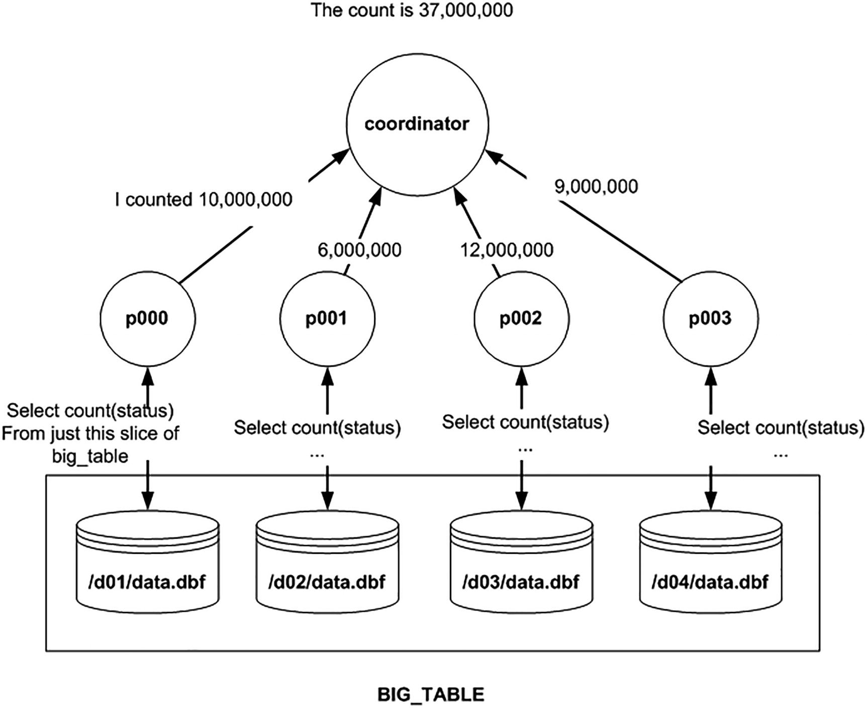
Parallel update (PDML) depiction

We can actually observe the fact that there are separate independent transactions created for the parallel execution servers. We’ll use two sessions again. In the session with SID=258, we explicitly enable parallel DML. PDML differs from parallel query in that regard; unless you explicitly ask for it, you will not get it:
$ sqlplus eoda/foo@PDB1
SQL> alter session enable parallel dml;
You can verify that parallel DML has been enabled for your session via
SQL> select pdml_enabled from v$session where sid = sys_context('userenv','sid');
PDM
---
YES

The fact that the table is “parallel” is not sufficient, as it was for parallel query. The reasoning behind the need to explicitly enable PDML in your session is the fact that PDML has certain limitations associated with it, which I list after this example.

In the same session, we do a bulk UPDATE that, because the table is “parallel enabled,” will in fact be done in parallel:
SQL> update big_table set status = 'done';
In the other session, we’ll join V$SESSION to V$TRANSACTION to show the active sessions for our PDML operation, as well as their independent transaction information:
SQL> select a.sid, a.program, b.start_time, b.used_ublk,
           b.xidusn ||'.'|| b.xidslot || '.' || b.xidsqn trans_id
      from v$session a, v$transaction b
     where a.taddr = b.addr
       and a.sid in ( select sid
                        from v$px_session
                       where qcsid = 258)
     order by sid;
  SID PROGRAM                      START_TIME           USED_UBLK TRANS_ID
----- ---------------------------- -------------------- --------- ---------
   17 sqlplus@orclvm (TNS V1-V3)   02/28/21 17:25:45            1 9.5.715
   19 oracle@orclvm (P000)         02/28/21 17:25:45            1 4.30.689
   20 oracle@orclvm (P006)         02/28/21 17:25:45        30903 6.4.720
  138 oracle@orclvm (P003)         02/28/21 17:25:45            1 2.9.718
  140 oracle@orclvm (P007)         02/28/21 17:25:45        29086 5.11.711
  253 oracle@orclvm (P001)         02/28/21 17:25:45            1 3.24.805
  260 oracle@orclvm (P004)         02/28/21 17:25:45        31386 7.4.693
  366 oracle@orclvm (P002)         02/28/21 17:25:45            1 1.31.707
  370 oracle@or (P005)             02/28/21 17:25:45        29114 8.4.766
9 rows selected
As you can see, there is a lot happening here. This is because the plan that was developed includes a step to update the table and independent steps to update the index entries. Look at a BASIC plus PARALLEL-enabled explain plan output from DBMS_XPLAN :
SQL> explain plan for update big_table set status = 'done';
Explained.
SQL> select * from table(dbms_xplan.display(null,null,'BASIC +PARALLEL'));
We see the following:
---------------------------------------------------------------------------
|  Id | Operation                | Name      |    TQ  |IN-OUT| PQ Distrib |
---------------------------------------------------------------------------
|   0 | UPDATE STATEMENT         |           |        |      |            |
|   1 |  PX COORDINATOR          |           |        |      |            |
|   2 |   PX SEND QC (RANDOM)    | :TQ10001  |  Q1,01 | P->S | QC (RAND)  |
|   3 |    INDEX MAINTENANCE     | BIG_TABLE |  Q1,01 | PCWP |            |
|   4 |     PX RECEIVE           |           |  Q1,01 | PCWP |            |
|   5 |      PX SEND RANGE       | :TQ10000  |  Q1,00 | P->P | RANGE      |
|   6 |       UPDATE             | BIG_TABLE |  Q1,00 | PCWP |            |
|   7 |        PX BLOCK ITERATOR |           |  Q1,00 | PCWC |            |
|   8 |         TABLE ACCESS FULL| BIG_TABLE |  Q1,00 | PCWP |            |
---------------------------------------------------------------------------
As a result of the pseudo-distributed implementation of PDML, certain limitations are associated with it:
  • Triggers are not supported during a PDML operation. This is a reasonable limitation in my opinion, since triggers tend to add a large amount of overhead to the update, and you are using PDML to go fast—the two features don’t go together.

  • There are certain declarative RI constraints that are not supported during the PDML, since each slice of the table is modified as a separate transaction in the separate session. Self-referential integrity is not supported, for example. Consider the deadlocks and other locking issues that would occur if it were supported.

  • You cannot access the table you’ve modified with PDML until you commit or roll back.

  • Advanced replication is not supported with PDML (because the implementation of advanced replication is trigger based).

  • Deferred constraints (i.e., constraints that are in the deferred mode) are not supported.

  • PDML may only be performed on tables that have bitmap indexes or LOB columns if the table is partitioned, and then the degree of parallelism would be capped at the number of partitions. You cannot parallelize an operation within partitions in this case, as each partition would get a single parallel execution server to operate on it. We should note that starting with Oracle 12c, you can run PDML on SecureFiles LOBs without partitioning.

  • Distributed transactions are not supported when performing PDML.

  • Clustered tables are not supported with PDML.

If you violate any of those restrictions, one of two things will happen: either the statement will be performed serially (no parallelism will be involved) or an error will be raised. For example, if you already performed the PDML against table T and then attempted to query table T before ending your transaction, then you will receive the error ORA-12838: cannot read/modify an object after modifying it in parallel.

It’s also worth noting in the prior example in this section that had you not enabled parallel DML for the UPDATE statement , then the explain plan output would look quite different, for example:
------------------------------------------------------------------------
| Id  | Operation             | Name      |    TQ  |IN-OUT| PQ Distrib |
------------------------------------------------------------------------
|   0 | UPDATE STATEMENT      |           |        |      |            |
|   1 |  UPDATE               | BIG_TABLE |        |      |            |
|   2 |   PX COORDINATOR      |           |        |      |            |
|   3 |    PX SEND QC (RANDOM)| :TQ10000  |  Q1,00 | P->S | QC (RAND)  |
|   4 |     PX BLOCK ITERATOR |           |  Q1,00 | PCWC |            |
|   5 |      TABLE ACCESS FULL| BIG_TABLE |  Q1,00 | PCWP |            |
------------------------------------------------------------------------

To the untrained eye, it may look like the UPDATE happened in parallel, but in fact it did not. What the prior output shows is that the UPDATE is serial and that the full scan (read) of the table was parallel. So there was parallel query involved, but no t PDML.

VERIFYING PARALLEL OPERATIONS
You can quickly verify the parallel operations that have occurred in a session by querying the data dictionary. For example, here’s a parallel DML operation:
SQL> alter session enable parallel dml;
SQL> update big_table set status='AGAIN';
Next, verify the type and number of parallel activities via
SQL> select name, value from v$statname a, v$mystat b
          where a.statistic# = b.statistic# and name like '%parallel%';
Here is some sample output for this session:
NAME                                                 VALUE
----------------------------------------------- ----------
DBWR parallel query checkpoint buffers written           0
queries parallelized                                     0
DML statements parallelized                              1
DDL statements parallelized                              0
DFO trees parallelized                                   1

The prior output verifies that one parallel DML statement has executed in this session.

Parallel DDL

I believe that parallel DDL is the real sweet spot of Oracle’s parallel technology. As we’ve discussed, parallel execution is generally not appropriate for OLTP systems. In fact, for many data warehouses, parallel query is becoming less and less of an option. It used to be that a data warehouse was built for a very small, focused user community—sometimes comprised of just one or two analysts. However, over the last decade or so, I’ve watched them grow from small user communities to user communities of hundreds or thousands. Consider a data warehouse front-ended by a web-based application: it could be accessible to literally thousands or more users simultaneously.

But a DBA performing the large batch operations, perhaps during a maintenance window, is a different story. The DBA is still a single individual, and they might have a huge machine with tons of computing resources available. The DBA has only one thing to do, such as load this data, or reorganize that table, or rebuild that index. Without parallel execution, the DBA would be hard-pressed to really use the full capabilities of the hardware. With parallel execution, they can. The following SQL DDL commands permit parallelization:
  • CREATE INDEX: Multiple parallel execution servers can scan the table, sort the data, and write the sorted segments out to the index structure.

  • CREATE TABLE AS SELECT: The query that executes the SELECT may be executed using parallel query, and the table load itself may be done in parallel.

  • ALTER INDEX REBUILD: The index structure may be rebuilt in parallel.

  • ALTER TABLE MOVE: A table may be moved in parallel.

  • ALTER TABLE SPLIT|COALESCE PARTITION: The individual table partitions may be split or coalesced in parallel.

  • ALTER INDEX SPLIT PARTITION: An index partition may be split in parallel.

  • CREATE/ALTER MATERIALIZED VIEW: Create a materialized view with parallel processes or change the default degree of parallelism.

Note

See the Oracle Database SQL Language Reference manual for a complete list of statements that support parallel operations.

The first four of these commands work for individual table/index partitions as well—that is, you may MOVE an individual partition of a table in parallel.

To me, parallel DDL is where the parallel execution in Oracle is of greatest measurable benefit. Sure, it can be used with parallel query to speed up certain long-running operations, but from a maintenance standpoint, and from an administration standpoint, parallel DDL is where the parallel operations affect us, DBAs and developers, the most. If you think of parallel query as being designed for the end user for the most part, then parallel DDL is designed for the DBA/developer.

Parallel DDL

Oracle provides the ability to perform parallel direct path loads, whereby multiple sessions can write directly to the Oracle datafiles, bypassing the buffer cache entirely, bypassing undo for the table data, and perhaps even bypassing redo generation. With parallel DDL or parallel DML plus external tables, we have a parallel direct path load that is implemented via a simple CREATE TABLE AS SELECT or INSERT /*+ APPEND */.

Let’s look at this in action. We’ll use the same BIG_TABLE from earlier, which is parallel enabled and contains ten million records. We’re going to join this to a second table, USER_INFO, which contains OWNER-related information from the ALL_USERS dictionary view. To start, we’ll create the USER_INFO table , enable it for parallel operations, and then gather statistics on it:
$ sqlplus eoda/foo@PDB1
SQL> create table user_info as select * from all_users;
Table created.
SQL> alter table user_info parallel;
Table altered.
SQL> exec dbms_stats.gather_table_stats( user, 'USER_INFO' );
PL/SQL procedure successfully completed.
Now, we would like to parallel direct path load a new table with this information. The query we’ll use is simply
SQL> create table new_table parallel as
          select a.*, b.user_id, b.created user_created
          from big_table a, user_info b
          where a.owner = b.username;
The plan for that particular CREATE TABLE AS SELECT statement looks like this:
---------------------------------------------------------------------------
| Id  | Operation                          | Name      |    TQ  |IN-OUT| PQ Distrib |
---------------------------------------------------------------------------
|   0 | CREATE TABLE STATEMENT             |           |        |      |            |
|   1 |  PX COORDINATOR                    |           |        |      |            |
|   2 |   PX SEND QC (RANDOM)              | :TQ10000  |  Q1,00 | P->S | QC (RAND)  |
|   3 |    LOAD AS SELECT (HYBRID TSM/HWMB)| NEW_TABLE |  Q1,00 | PCWP |            |
|   4 |     OPTIMIZER STATISTICS GATHERING |           |  Q1,00 | PCWP |            |
|   5 |      HASH JOIN                     |           |  Q1,00 | PCWP |            |
|   6 |       TABLE ACCESS FULL            | USER_INFO |  Q1,00 | PCWP |            |
|   7 |       PX BLOCK ITERATOR            |           |  Q1,00 | PCWC |            |
|   8 |        TABLE ACCESS FULL           | BIG_TABLE |  Q1,00 | PCWP |            |
---------------------------------------------------------------------------

If you look at the steps from 5 on down, this is the query (SELECT) component. The scan of BIG_TABLE and hash join to USER_INFO was performed in parallel, and each of the subresults was loaded into a portion of the table (step 3, the LOAD AS SELECT). After each of the parallel execution servers finished its part of the join and load, it sent its results up to the query coordinator. In this case, the results simply indicated “success” or “failure,” as the work had already been performed.

And that is all there is to it—parallel direct path loads made easy. The most important thing to consider with these operations is how space is used (or not used). Of particular importance is a side effect called extent trimming. Let’s spend some time investigating that now.

Parallel DDL and Extent Trimming

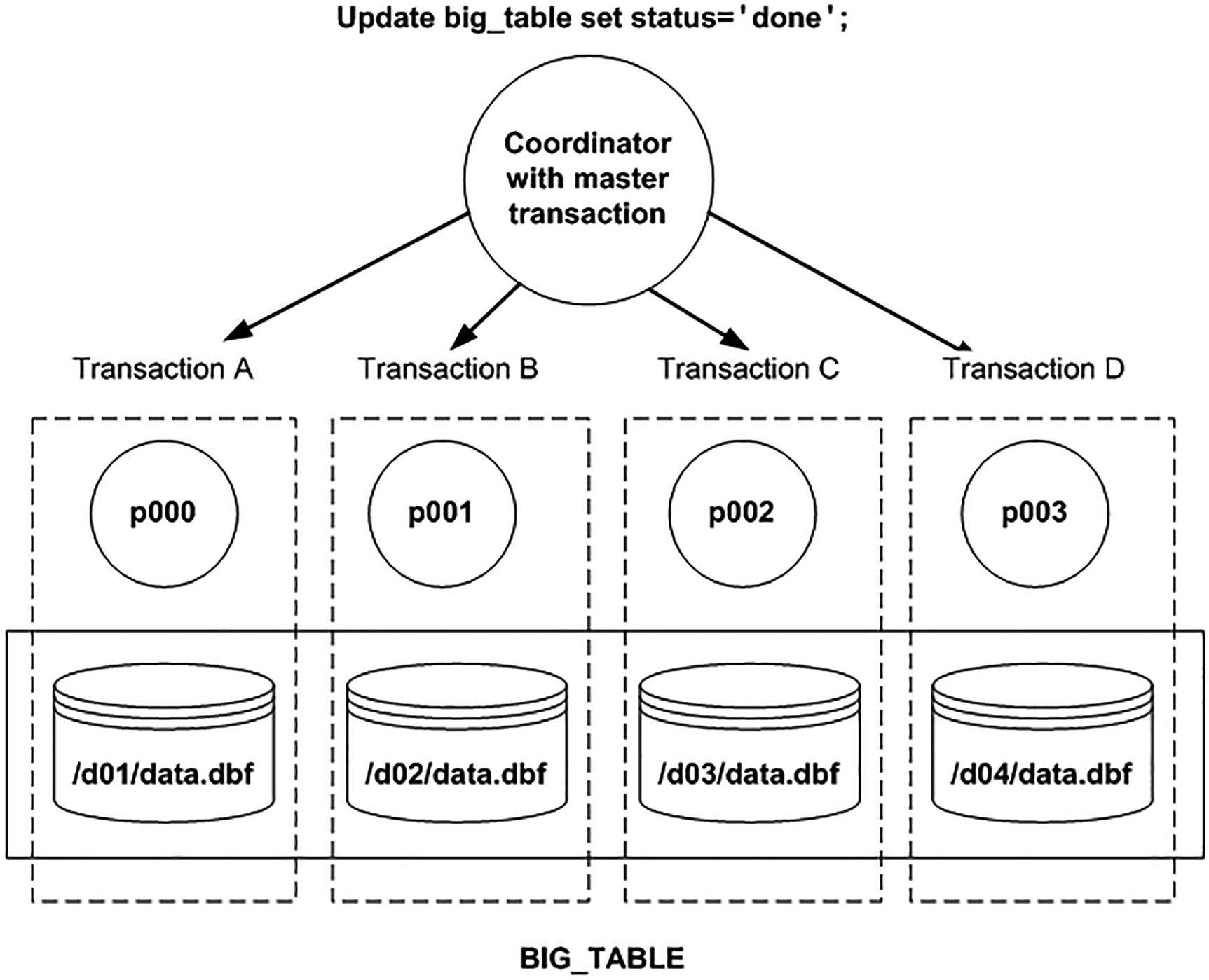
Parallel DDL relies on direct path operations. That is, the data is not passed to the buffer cache to be written later; rather, an operation such as a CREATE TABLE AS SELECT will create new extents and write directly to them, and the data goes straight from the query to disk in those newly allocated extents. Each parallel execution server performing its part of the CREATE TABLE AS SELECT will write to its own extent. The INSERT /*+ APPEND */ (a direct path insert) writes “above” a segment’s high-water mark (HWM), and each parallel execution server will again write to its own set of extents, never sharing them with other parallel execution servers. Therefore, if you do a parallel CREATE TABLE AS SELECT and use four parallel execution servers to create the table, then you will have at least four extents—maybe more. But each of the parallel execution servers will allocate its own extent, write to it, and, when it fills up, allocate another new extent. The parallel execution servers will never use an extent allocated by some other parallel execution server.

Figure 14-3 depicts this process. We have a CREATE TABLE NEW_TABLE AS SELECT being executed by four parallel execution servers. In the figure, each parallel execution server is represented by a different color. The boxes in the disk drum represent the extents that were created in some datafile by this CREATE TABLE statement. Each extent is presented in a different color, for the simple reason that all of the data in any given extent was loaded by only one of the four parallel execution servers—for example, p003 is depicted as having created and then loaded four of these extents, and so on.
../images/319655_4_En_14_Chapter/319655_4_En_14_Fig3_HTML.jpg
Figure 14-3

Parallel DDL extent allocation depiction

This sounds all right at first, but in a data warehouse environment, this can lead to wastage after a large load. Let’s say you want to load 1010MB of data (about 1GB), and you are using a tablespace with 100MB extents. You decide to use ten parallel execution servers to load this data. Each would start by allocating its own 100MB extent (there will be ten of them in all) and filling it up. Since each has 101MB of data to load, they would fill up their first extent and then proceed to allocate another 100MB extent, of which they would use 1MB. You now have 20 extents (10 of which are full, and 10 of which have 1MB each), and the remaining 990MB is “allocated but not used.” This space could be used the next time you load more data, but right now you have 990MB of dead space. This is where extent trimming comes in. Oracle will attempt to take the last extent of each parallel execution server and trim it back to the smallest size possible.

Extent Trimming and Locally Managed Tablespaces

Enter locally managed tablespaces. There are two types: UNIFORM SIZE, whereby every extent in the tablespace is always precisely the same size, and AUTOALLOCATE, whereby Oracle decides how big each extent should be using an internal algorithm. Both of these approaches nicely solve the 99MB of free space/followed by 1MB of used space/followed by 99MB of free space problem. However, they each solve it very differently. The UNIFORM SIZE approach obviates extent trimming from consideration all together. When you use UNIFORM SIZEs, Oracle cannot perform extent trimming. All extents are of that single size—none can be smaller (or larger) than that single size. AUTOALLOCATE extents, on the other hand, do support extent trimming, but in an intelligent fashion. They use a few specific sizes of extents and have the ability to use space of different sizes—that is, the algorithm permits the use of all free space over time in the tablespace. Unlike the dictionary-managed tablespace, where if you request a 100MB extent, Oracle will fail the request if it can find only 99MB free extents (so close, yet so far), a locally managed tablespace with AUTOALLOCATE extents can be more flexible. It may reduce the size of the request it was making in order to attempt to use all of the free space.

Let’s now look at the differences between the two locally managed tablespace approaches. To do that, we need a real-life example to work with. We’ll set up an external table capable of being used in a parallel direct path load situation, which is something that we do frequently. Even if you are still using SQL*Loader to parallel direct path load data, this section applies entirely—you just have manual scripting to do to actually load the data. So, in order to investigate extent trimming, we need to set up our example load and then perform the loads under varying conditions and examine the results.

Setting Up for Locally Managed Tablespaces

To get started, we need an external table. I’ve found time and time again that I have a legacy control file from SQL*Loader that I used to use to load data, one that looks like this, for example:
LOAD DATA
INFILE '/tmp/big_table.dat'
INTO TABLE big_table
REPLACE
FIELDS TERMINATED BY '|'
( id ,owner ,object_name ,subobject_name ,object_id
,data_object_id ,object_type ,created ,last_ddl_time
,timestamp ,status ,temporary ,generated ,secondary
,namespace ,edition_name
)
We can convert this easily into an external table definition using SQL*Loader itself:
$ sqlldr eoda/foo@PDB1 big_table.ctl external_table=generate_only
...
Path used:      External Table
Note

If you are curious about the SQLLDR command and the options used with it, we’ll be covering that in detail in the next chapter.

You should have a big_table.log file in your current working directory. Open it up. Notice the parameter EXTERNAL_TABLE passed to SQL*Loader. It causes SQL*Loader, in this case, to not load data, but rather to generate a CREATE TABLE statement for us in the log file. This CREATE TABLE statement looked as follows (this is an abridged form; I’ve edited out repetitive elements to make the example smaller):
CREATE TABLE "SYS_SQLLDR_X_EXT_BIG_TABLE"
(
  "ID" NUMBER,
  "OWNER" VARCHAR2(128),
  "OBJECT_NAME" VARCHAR2(128),
  "SUBOBJECT_NAME" VARCHAR2(128),
  "OBJECT_ID" NUMBER,
  "DATA_OBJECT_ID" NUMBER,
  "OBJECT_TYPE" VARCHAR2(23),
  "CREATED" DATE,
  "LAST_DDL_TIME" DATE,
  "TIMESTAMP" VARCHAR2(19),
  "STATUS" VARCHAR2(7),
  "TEMPORARY" VARCHAR2(1),
  "GENERATED" VARCHAR2(1),
  "SECONDARY" VARCHAR2(1),
  "NAMESPACE" NUMBER,
  "EDITION_NAME" VARCHAR2(128)
)
ORGANIZATION external
(
  TYPE oracle_loader
  DEFAULT DIRECTORY SYS_SQLLDR_XT_TMPDIR_00000
  ACCESS PARAMETERS
  (
    RECORDS DELIMITED BY NEWLINE CHARACTERSET US7ASCII
    BADFILE 'SYS_SQLLDR_XT_TMPDIR_00001':'big_table.bad'
    LOGFILE 'SYS_SQLLDR_XT_TMPDIR_00001':'big_table.log_xt'
    READSIZE 1048576
    FIELDS TERMINATED BY "|" LDRTRIM
...
      "EDITION_NAME" CHAR(255)
        TERMINATED BY "|"
    )
  )
  location
  (
    'big_table.dat'
  )
)REJECT LIMIT UNLIMITED
All we need to do is edit it to name the external table the way we want, perhaps change the directories, and so on:
$ sqlplus eoda/foo@PDB1
SQL> create or replace directory my_dir as '/tmp/';
And after that, all we need to do is actually create the external table:
CREATE TABLE BIG_TABLE_ET
(
  "ID" NUMBER,
  "OWNER" VARCHAR2(128),
  "OBJECT_NAME" VARCHAR2(128),
  "SUBOBJECT_NAME" VARCHAR2(128),
  "OBJECT_ID" NUMBER,
  "DATA_OBJECT_ID" NUMBER,
  "OBJECT_TYPE" VARCHAR2(23)
)
ORGANIZATION external
(
  TYPE oracle_loader
  DEFAULT DIRECTORY my_dir
  ACCESS PARAMETERS
  (
    RECORDS DELIMITED BY NEWLINE CHARACTERSET US7ASCII
    READSIZE 1048576
    FIELDS TERMINATED BY "|" LDRTRIM
    REJECT ROWS WITH ALL NULL FIELDS
    (
      "ID" CHAR(255)
        TERMINATED BY "|",
      "OWNER" CHAR(255)
        TERMINATED BY "|",
      "OBJECT_NAME" CHAR(255)
        TERMINATED BY "|",
      "SUBOBJECT_NAME" CHAR(255)
        TERMINATED BY "|",
      "OBJECT_ID" CHAR(255)
        TERMINATED BY "|",
      "DATA_OBJECT_ID" CHAR(255)
        TERMINATED BY "|",
      "OBJECT_TYPE" CHAR(255)
        TERMINATED BY "|"
    )
  )
  location
  (
    'big_table.dat'
  )
)REJECT LIMIT UNLIMITED parallel;
Table created.
Then we make this table parallel enabled. This is the magic step—this is what will facilitate an easy parallel direct path load:
SQL> alter table big_table_et PARALLEL;
Table altered.
Note

The PARALLEL clause is also used on the CREATE TABLE statement itself. Right after the REJECT LIMIT UNLIMITED, the keyword PARALLEL is added. I used the ALTER statement just to draw attention to the fact that the external table is, in fact, parallel enabled.

Extent Trimming with UNIFORM vs. AUTOALLOCATE Locally Managed Tablespaces

That’s all we need to do with regard to setting up the load component. Now, we would like to investigate how space is managed in a locally managed tablespace (LMT) that uses UNIFORM extent sizes, compared to how space is managed in an LMT that AUTOALLOCATEs extents. In this case, we’ll use 100MB extents. First, we create a tablespace called LMT_UNIFORM, which uses uniform extent sizes:
$ sqlplus eoda/foo@PDB1
SQL> create tablespace lmt_uniform
datafile '/opt/oracle/oradata/CDB/PDB1/uniform.dbf'
size 1048640K reuse
autoextend on next 100m
extent management local
UNIFORM SIZE 100m;
Next, we create a tablespace named LMT_AUTO, which uses AUTOALLOCATE to determine extent sizes:
SQL> create tablespace lmt_auto
datafile '/opt/oracle/oradata/CDB/PDB1/auto.dbf'
size 1048640K reuse
autoextend on next 100m
extent management local
AUTOALLOCATE;

Each tablespace started with a 1GB datafile (plus 64KB used by locally managed tablespaces to manage the storage; it would be 128KB extra instead of 64KB if we were to use a 32KB block size). We permit these datafiles to autoextend 100MB at a time.

For the setup for this exercise, the BIG_TABLE table was created with 10,000,000 rows using the big_table.sql script found in the “Setting Up Your Environment” section at the beginning of this book. And then the table was easily unloaded into a CSV file as follows:
SQL> set verify off feedback off termout off echo off trimspool on pagesize 0 head off
SQL> set markup csv on quote off delimiter |
SQL> spo /tmp/big_table.dat
SQL> select * from big_table;
SQL> spo off;
We are going to load the file we just created, which is a 10,000,000-record file:
$  ls -lag /tmp/big_table.dat
- -rw-r--r--. 1 oinstall 1407984520 May 22 19:03 /tmp/big_table.dat
Next, we do a parallel direct path load of this file into each tablespace:
SQL> create table uniform_test  parallel
    tablespace lmt_uniform
    as select * from big_table_et;
Table created.
SQL> create table autoallocate_test parallel
    tablespace lmt_auto  as
    select * from big_table_et;
Table created.
On my four-CPU system, these CREATE TABLE statements executed with several parallel execution servers and one coordinator. I verified this by querying one of the dynamic performance views related to parallel execution, V$PX_SESSION, while these statements were running:
SQL> select sid, serial#, qcsid, qcserial#, degree from v$px_session;
SID      SERIAL#      QCSID  QCSERIAL#     DEGREE
----- ---------- ---------- ---------- ----------
   19      57630         21      25039          4
  253      14721         21      25039          4
  370      58100         21      25039          4
  140      64104         21      25039          4
   21      25039         21
Note

In creating the UNIFORM_TEST and AUTOALLOCATE_TEST tables, we simply specified “parallel” on each table, with Oracle choosing the degree of parallelism. In this case, I was the sole user of the machine (all resources available), and Oracle defaulted it to four based on the number of CPUs (four) and the PARALLEL_THREADS_PER_CPU parameter setting, which is one. For your system, you may have different settings and therefore execute with a different degree of parallelism.

The SID,SERIAL# are the identifiers of the parallel execution sessions, and the QCSID,QCSERIAL# is the identifier of the query coordinator of the parallel execution. So, with parallel execution sessions running, we would like to see how the space was used. A quick query against USER_SEGMENTS gives us a good idea:
SQL> select segment_name, blocks, extents  from user_segments
    where segment_name in ( 'UNIFORM_TEST', 'AUTOALLOCATE_TEST' );
SEGMENT_NAME                  BLOCKS    EXTENTS
------------------------- ---------- ----------
AUTOALLOCATE_TEST             102936        101
UNIFORM_TEST                  115200          9
Since we were using an 8KB block size, this shows a difference of about 100MB; looking at it from a ratio perspective, AUTOALLOCATE_TEST is about 90 percent the size of UNIFORM_TEST as far as allocated space goes. The actual used space results are as follows:
SQL> set serverout on;
SQL> exec show_space('UNIFORM_TEST' );
Unformatted Blocks .....................               0
FS1 Blocks (0-25)  .....................               0
FS2 Blocks (25-50) .....................               0
FS3 Blocks (50-75) .....................               0
FS4 Blocks (75-100).....................               0
Full Blocks        .....................         102,442
Total Blocks............................         115,200
Total Bytes.............................     943,718,400
Total MBytes............................             900
Unused Blocks...........................          12,305
Unused Bytes............................     100,802,560
Last Used Ext FileId....................              13
Last Used Ext BlockId...................         102,528
Last Used Block.........................             495
SQL> exec show_space('AUTOALLOCATE_TEST' );
Unformatted Blocks .....................               0
FS1 Blocks (0-25)  .....................               0
FS2 Blocks (25-50) .....................               0
FS3 Blocks (50-75) .....................               0
FS4 Blocks (75-100).....................               3
Full Blocks        .....................         102,442
Total Blocks............................         102,936
Total Bytes.............................     843,251,712
Total MBytes............................             804
Unused Blocks...........................               0
Unused Bytes............................               0
Last Used Ext FileId....................              14
Last Used Ext BlockId...................         102,528
Last Used Block.........................             536
Note

The SHOW_SPACE procedure is described in the “Setting Up Your Environment” section at the beginning of this book.

Notice that the autoallocated table shows 843MB used space vs. 943MB used for the uniform extent table. This is all due to the extent trimming that did not take place. If we look at UNIFORM_TEST , we see this clearly:
SQL> select segment_name, extent_id, blocks from user_extents where segment_name = 'UNIFORM_TEST';
SEGMENT_NAME               EXTENT_ID     BLOCKS
------------------------- ---------- ----------
UNIFORM_TEST                       0      12800
UNIFORM_TEST                       1      12800
UNIFORM_TEST                       2      12800
UNIFORM_TEST                       3      12800
UNIFORM_TEST                       4      12800
UNIFORM_TEST                       5      12800
UNIFORM_TEST                       6      12800
UNIFORM_TEST                       7      12800
UNIFORM_TEST                       8      12800
9 rows selected.
Each extent is 100MB in size. Now, it would be a waste of paper to list all 100 plus extents allocated to the AUTOALLOCATE_TEST tablespace , so let’s look at them in aggregate:
SQL> select segment_name, blocks, count(*)
    from user_extents
    where segment_name = 'AUTOALLOCATE_TEST'
    group by segment_name, blocks
    order by blocks;
SEGMENT_NAME                  BLOCKS   COUNT(*)
------------------------- ---------- ----------
AUTOALLOCATE_TEST                536          1
AUTOALLOCATE_TEST               1024        100

This generally fits in with how locally managed tablespaces with AUTOALLOCATE are observed to allocate space (the results of the prior query will vary depending on the amount of data and the version of Oracle). Values such as the 1024 and 8192 block extents are normal; we will observe them all of the time with AUTOALLOCATE. Other values are not normal; we do not usually observe them. They are due to the extent trimming that takes place. Some of the parallel execution servers finished their part of the load—they took their last 64MB (1024 blocks) extent and trimmed it, resulting in a spare bit left over. One of the other parallel execution sessions, as it needed space, could use this spare bit. In turn, as these other parallel execution sessions finished processing their own loads, they would trim their last extent and leave spare bits of space.

So, which approach should you use? If your goal is to direct path load in parallel as often as possible, I suggest AUTOALLOCATE as your extent management policy. Parallel direct path operations like this will not use space under the object’s HWM—the space on the freelist. So, unless you do some conventional path inserts into these tables also, UNIFORM allocation will permanently have additional free space in it that it will never use. Unless you can size the extents for the UNIFORM locally managed tablespace to be much smaller, you will see what I would term excessive wastage over time, and remember that this space is associated with the segment and will be included in a full scan of the table.

To demonstrate this, let’s do another parallel direct path load into these existing tables, using the same inputs:
SQL> alter session enable parallel dml;
Session altered.
SQL> insert /*+ append */ into UNIFORM_TEST select * from big_table_et;
10000000 rows created.
SQL> insert /*+ append */ into AUTOALLOCATE_TEST select * from big_table_et;
10000000 rows created.
SQL> commit;
Commit complete.
If we compare the space utilization of the two tables after that operation, as follows, we can see that as we load more and more data into the table UNIFORM_TEST using parallel direct path operations, the space utilization gets worse over time:
SQL> exec show_space( 'UNIFORM_TEST' );
Unformatted Blocks .....................               0
FS1 Blocks (0-25)  .....................               0
FS2 Blocks (25-50) .....................               0
FS3 Blocks (50-75) .....................               0
FS4 Blocks (75-100).....................          24,610
Full Blocks        .....................         204,884
Total Blocks............................         230,400
Total Bytes.............................   1,887,436,800
Total MBytes............................           1,800
Unused Blocks...........................               0
Unused Bytes............................               0
Last Used Ext FileId....................              13
Last Used Ext BlockId...................         217,728
Last Used Block.........................          12,800
SQL> exec show_space( 'AUTOALLOCATE_TEST' );
Unformatted Blocks .....................               0
FS1 Blocks (0-25)  .....................               0
FS2 Blocks (25-50) .....................               0
FS3 Blocks (50-75) .....................               0
FS4 Blocks (75-100).....................               4
Full Blocks        .....................         204,886
Total Blocks............................         205,872
Total Bytes.............................   1,686,503,424
Total MBytes............................           1,608
Unused Blocks...........................               0
Unused Bytes............................               0
Last Used Ext FileId....................              14
Last Used Ext BlockId...................         205,568
Last Used Block.........................             536

We would want to use a significantly smaller uniform extent size or use the AUTOALLOCATE clause. The AUTOALLOCATE clause may well generate more extents over time, but the space utilization is superior due to the extent trimming that takes place.

Note

I noted earlier in this chapter that your mileage may vary when executing the prior parallelism examples. It’s worth highlighting this point again; your results will vary depending on the version of Oracle, the degree of parallelism used, and the amount of data loaded. The prior output in this section was generated using the latest release of Oracle 21c with the default degree of parallelism on a four-CPU box.

Procedural Parallelism

I would like to discuss two types of procedural parallelism:
  • Parallel pipelined functions, which is a feature of Oracle

  • Do-it-yourself (DIY) parallelism, which is the application to your own applications of the same techniques that Oracle applies to parallel full table scans

Often, you’ll find that applications—typically batch processes—designed to execute serially will look something like the following procedure:
Create procedure process_data
As
Begin
For x in ( select * from some_table )
   Perform complex process on X
   Update some other table, or insert the record somewhere else
End loop
end

In this case, Oracle’s parallel query or PDML won’t help a bit (in fact, parallel execution of the SQL by Oracle here would likely only cause the database to consume more resources and take longer). If Oracle were to execute the simple SELECT * FROM SOME_TABLE in parallel, it would provide this algorithm no apparent increase in speed whatsoever. If Oracle were to perform in parallel the UPDATE or INSERT after the complex process, it would have no positive effect (it is a single-row UPDATE/INSERT, after all).

There is one obvious thing you could do here: use array processing for the UPDATE/INSERT after the complex process. However, that isn’t going to give you a 50 percent reduction or more in runtime, which is often what you’re looking for. Don’t get me wrong, you definitely want to implement array processing for the modifications here, but it won’t make this process run two, three, four, or more times faster.

Now, suppose this process runs at night on a machine with four CPUs, and it is the only activity taking place. You have observed that only one CPU is partially used on this system, and the disk system is not being used very much at all. Further, this process is taking hours, and every day it takes a little longer as more data is added. You need to reduce the runtime dramatically—it needs to run four or eight times faster—so incremental percentage increases will not be sufficient. What can you do?

There are two approaches you can take. One approach is to implement a parallel pipelined function, whereby Oracle will decide on appropriate degrees of parallelism (assuming you have opted for that, which would be recommended). Oracle will create the sessions, coordinate them, and run them, very much like the previous example with parallel DDL or parallel DML where, by using CREATE TABLE AS SELECT or INSERT /*+ APPEND */, Oracle fully automated parallel direct path loads for us. The other approach is DIY parallelism. We’ll take a look at both approaches in the sections that follow.

Parallel Pipelined Functions

We’d like to take that very serial process PROCESS_DATA from earlier and have Oracle execute it in parallel for us. To accomplish this, we need to turn the routine inside out. Instead of selecting rows from some table, processing them, and inserting them into another table, we will insert into another table the results of fetching some rows and processing them. We will remove the INSERT at the bottom of that loop and replace it in the code with a PIPE ROW clause. The PIPE ROW clause allows our PL/SQL routine to generate table data as its output, so we’ll be able to SELECT from our PL/SQL process. The PL/SQL routine that used to procedurally process the data becomes a table, in effect, and the rows we fetch and process are the outputs. We’ve seen this many times throughout this book every time we’ve issued the following:
Select * from table(dbms_xplan.display);

That is a PL/SQL routine that reads the PLAN_TABLE; restructures the output, even to the extent of adding rows; and then outputs this data using PIPE ROW to send it back to the client. We’re going to do the same thing here, in effect, but we’ll allow for it to be processed in parallel.

We’re going to use two tables in this example: T1 and T2. T1 is the table we were reading previously in the select * from some_table line of the PROCESS_DATA procedure ; T2 is the table we need to move this information into. Assume this is some sort of ETL process we run to take the transactional data from the day and convert it into reporting information for tomorrow. The two tables we’ll use are as follows:
SQL> create table t1 as select object_id id, object_name text from all_objects;
Table created.
SQL> exec dbms_stats.set_table_stats( user, 'T1', numrows=>10000000,numblks=>100000 );
PL/SQL procedure successfully completed.
SQL> create table t2 as select t1.*, 0 session_id from t1 where 1=0;
Table created.

We used DBMS_STATS to trick the optimizer into thinking that there are 10,000,000 rows in that input table and that it consumes 100,000 database blocks. We want to simulate a big table here. The second table, T2, is a copy of the first table’s structure with the addition of a SESSION_ID column. That column will be useful to actually see the parallelism that takes place.

Next, we need to set up object types for our pipelined function to return. The object type is a structural definition of the output of the procedure we are converting. In this case, it looks just like T2:
SQL> CREATE OR REPLACE TYPE t2_type
    AS OBJECT (
     id         number,
     text       varchar2(4000),
     session_id number
    )
  /
Type created.
SQL> create or replace type t2_tab_type
    as table of t2_type
    /
Type created.

And now for the pipelined function, which is simply the original PROCESS_DATA procedure rewritten. The procedure is now a function that produces rows. It accepts as an input the data to process in a ref cursor. The function returns a T2_TAB_TYPE, the type we just created. It is a pipelined function that is PARALLEL_ENABLED. The partition clause we are using says to Oracle, “Partition, or slice up, the data by any means that works best. We don’t need to make any assumptions about the order of the data.”

You may also use hash or range partitioning on a specific column in the ref cursor. This would involve using a strongly typed ref cursor, so the compiler knows what columns are available. Hash partitioning would just send equal rows to each parallel execution server to process based on a hash of the column supplied. Range partitioning would send nonoverlapping ranges of data to each parallel execution server, based on the partitioning key. For example, if you range partitioned on ID, each parallel execution server might get ranges 1–1000, 1001–20000, 20001–30000, and so on (ID values in that range).

Here, we just want the data split up. How the data is split up is not relevant to our processing, so our definition looks like this:

Note

Ensure the user you’re using has been granted select on sys.v_$mystat in the pluggable database that you’re connected to before attempting to create this next procedure.

SQL> create or replace
    function parallel_pipelined( l_cursor in sys_refcursor )
    return t2_tab_type
    pipelined
    parallel_enable ( partition l_cursor by any )
We’d like to be able to see what rows were processed by which parallel execution servers, so we’ll declare a local variable L_SESSION_ID and initialize it from V$MYSTAT :
    is
        l_session_id number;
        l_rec        t1%rowtype;
  begin
      select sid into l_session_id
        from v$mystat
       where rownum =1;
Now we are ready to process the data. We simply fetch out a row (or rows, as we could certainly use BULK COLLECT here to array process the ref cursor), perform our complex process on it, and pipe it out. When the ref cursor is exhausted of data, we close the cursor and return:
      loop
          fetch l_cursor into l_rec;
          exit when l_cursor%notfound;
          -- complex process here
          pipe row(t2_type(l_rec.id,l_rec.text,l_session_id));
      end loop;
      close l_cursor;
      return;
  end;
  /
Function created.
And that’s it. We’re ready to process the data in parallel, letting Oracle figure out based on the resources available what the most appropriate degree of parallelism is:
SQL> alter session enable parallel dml;
Session altered.
SQL> insert /*+ append */ into t2(id,text,session_id)
    select * from table(parallel_pipelined
              (CURSOR(select /*+ parallel(t1) */ *
                        from t1 )
               ));
17914 rows created.
SQL> commit;
Commit complete.
Just to see what happened here, we can query the newly inserted data out and group by SESSION_ID to see how many parallel execution servers were used and how many rows each one processed:
SQL> select session_id, count(*)  from t2 group by session_id;
SESSION_ID   COUNT(*)
---------- ----------
       366      14253
       140      16188
       251      15693
        19      20983

Apparently, we used four parallel execution servers for the SELECT component of this parallel operation, and each one processed about 16,000 records each. Your results may vary depending on the number of CPUs on your system and version of Oracle.

As you can see, Oracle parallelized our process, but we underwent a fairly radical rewrite of our process. This is a long way from the original implementation. So, while Oracle can process our routine in parallel, we may well not have any routines that are coded to be parallelized. If a rather large rewrite of your procedure is not feasible, you may well be interested in the next implementation: DIY parallelism.

Do-It-Yourself Parallelism

Say we have that same process as in the preceding section: the serial, simple procedure. We cannot afford a rather extensive rewrite of the implementation, but we would like to execute it in parallel. What can we do?

Oracle has a mechanism to implement parallelism via the DBMS_PARALLEL_EXECUTE built-in package. Using it, you can execute a SQL or PL/SQL statement in parallel by taking the data to be processed and breaking it up into multiple, smaller streams. The beauty of this package is that it eliminates much of the tedious work that you otherwise need to perform.

Let’s start with the premise that we have a SERIAL routine that we’d like to execute in parallel against some large table. We’d like to do it with as little work as possible; in other words, modify as little code as possible and be responsible for generating very little new code. Enter DBMS_PARALLEL_EXECUTE . We will not cover every possible use of this package (it is fully documented in the Oracle Database PL/SQL Packages and Types Reference manual) but we will use just enough of it to implement the process I’ve just described.

Assuming we start with the empty table T2, we’ll modify our serial process now to look like this:
$ sqlplus eoda/foo@PDB1
SQL> create or replace
    procedure serial( p_lo_rid in rowid, p_hi_rid in rowid )
    is
    begin
        for x in ( select object_id id, object_name text
                     from big_table
                    where rowid between p_lo_rid
                                    and p_hi_rid )
        loop
          -- complex process here
          insert into t2 (id, text, session_id )
          values ( x.id, x.text, sys_context( 'userenv', 'sessionid' ) );
      end loop;
  end;
 /
Procedure created.

That’s it: just add the ROWID inputs and the predicate. The modified code has not changed much at all. I am using SYS_CONTEXT to get the SESSIONID so we can monitor how much work was done by each thread, each parallel session.

Now, to start the process, we first need to break up the table into small pieces. We can do this by some numeric range—useful for tables that use a SEQUENCE to populate their primary key, by any arbitrary SQL you want to code or by ROWID ranges . We’ll use the ROWID range. I find it to be the most efficient because it creates nonoverlapping ranges of the table (contention free) and doesn’t require querying the table to decide the ranges; it just uses the data dictionary. So, we’ll make the following API calls:
SQL> begin
        dbms_parallel_execute.create_task('PROCESS BIG TABLE');
        dbms_parallel_execute.create_chunks_by_rowid
        ( task_name   => 'PROCESS BIG TABLE',
          table_owner => user,
          table_name  => 'BIG_TABLE',
          by_row      => false,
          chunk_size  => 10000 );
    end;
 /
PL/SQL procedure successfully completed.

We started by creating a named task: 'PROCESS BIG TABLE' in this case. This is just a unique name we’ll use to refer to our big process. Second, we invoked the CREATE_CHUNKS_BY_ROWID procedure. This procedure does exactly what its name implies: it “chunks up” a table by ROWID ranges in a manner similar to what we just did. We told the procedure to read the information about the currently logged in user’s table named BIG_TABLE and to break it up into chunks of no more than about 10,000 blocks (CHUNK_SIZE). The parameter BY_ROW was set to false which implies, in this case, that the CHUNK_SIZE is not a count of rows to create ROWID ranges by but rather a count of blocks to create them.

We can see the number of chunks and information about each chunk immediately after this block of code executes by querying DBA_PARALLEL_EXECUTE_CHUNKS :
SQL> select *  from (
    select chunk_id, status, start_rowid, end_rowid
      from dba_parallel_execute_chunks
     where task_name = 'PROCESS BIG TABLE'
     order by chunk_id
           )
     where rownum <= 5;
  CHUNK_ID STATUS               START_ROWID        END_ROWID
---------- -------------------- ------------------ ------------------
         1 UNASSIGNED           AAAR1MAAMAAAACAAAA AAAR1MAAMAAACePH//
         2 UNASSIGNED           AAAR1MAAMAAACeQAAA AAAR1MAAMAAAE6fH//
         3 UNASSIGNED           AAAR1MAAMAAAE6gAAA AAAR1MAAMAAAHWvH//
         4 UNASSIGNED           AAAR1MAAMAAAHWwAAA AAAR1MAAMAAAJy/H//
         5 UNASSIGNED           AAAR1MAAMAAAJzAAAA AAAR1MAAMAAAMPPH//
The query in this example shows the first five rows in the view; in my case, there were 18 total rows in there for the table in question, each representing a nonoverlapping chunk of the table to process. This does not mean we’ll be processing the table in “parallel 18,” just that we have 118 chunks in total to process. We are now ready to run our task via this API call:
SQL> begin
        dbms_parallel_execute.run_task
        ( task_name      => 'PROCESS BIG TABLE',
          sql_stmt       => 'begin serial( :start_id, :end_id ); end;',
          language_flag  => DBMS_SQL.NATIVE,
          parallel_level => 4 );
    end;
  /
PL/SQL procedure successfully completed.

Here, we asked to run our task 'PROCESS BIG TABLE'—which points to our chunks. The SQL statement we want to execute is 'begin serial( :start_id, :end_id ); end;'—a simple call to our stored procedure with the ROWID range to process. The PARALLEL_LEVEL I decided to use was four, meaning we’ll have four parallel threads/processes executing this. Even though there were 218 chunks, we’ll only do four at a time. Internally, this package uses the DBMS_SCHEDULER package to run these threads in parallel.

Once our task starts running, it will create four jobs; each job is told to process the chunks identified by the key value 'PROCESS BIG TABLE' and run the stored procedure SERIAL against each chunk. So, these four sessions start, and each reads a chunk from the DBA_PARALLEL_EXECUTE_CHUNKS view, processes it, and updates the STATUS column. If the chunk is successful, the row will be marked as PROCESSED; if it fails for any reason or if a given chunk cannot be processed, it will be marked as PROCESSED_WITH_ERROR, and other columns will contain the detailed error message indicating the cause of the error. In either case, the session will then retrieve another chunk and process it and so on. So, eventually these four jobs will have processed all of the chunks, and the task will complete.

If any of the chunks failed, you can correct the underlying cause of the error and resume the task. This will cause it to reprocess the failed chunks. When all complete successfully, you are done.
SQL> select *  from (
    select chunk_id, status, start_rowid, end_rowid
      from dba_parallel_execute_chunks
      where task_name = 'PROCESS BIG TABLE'
     order by chunk_id
           )
     where rownum <= 5;
  CHUNK_ID STATUS               START_ROWID        END_ROWID
---------- -------------------- ------------------ ------------------
         1 PROCESSED            AAAR1MAAMAAAACAAAA AAAR1MAAMAAACePH//
         2 PROCESSED            AAAR1MAAMAAACeQAAA AAAR1MAAMAAAE6fH//
         3 PROCESSED            AAAR1MAAMAAAE6gAAA AAAR1MAAMAAAHWvH//
         4 PROCESSED            AAAR1MAAMAAAHWwAAA AAAR1MAAMAAAJy/H//
         5 PROCESSED            AAAR1MAAMAAAJzAAAA AAAR1MAAMAAAMPPH//
You can either retain the task for history or remove it. The following example shows how to remove the task:
SQL> begin
          dbms_parallel_execute.drop_task('PROCESS BIG TABLE' );
    end;
  /
PL/SQL procedure successfully completed.
If we review our own application table, we can see that the job was done using parallel 4, and each of the four processed about the same number of rows:
SQL> select session_id, count(*) from t2  group by session_id order by session_id;
SESSION_ID   COUNT(*)
---------- ----------
     22603    2521812
     22604    2485273
     22605    2529386
     22606    2463529
4 rows selected.

The DBMS_PARALLEL_EXECUTE package provides a rich API (which we’ve just touched on here). If you need to process in parallel, then you should familiarize yourself with this package.

Old-School Do-It-Yourself Parallelism

You can also manually implement parallelism. My approach many times has been to use rowid ranges to break the table up into some number of ranges that don’t overlap (yet completely cover the table).

Note

See the previous section for an example using the DBMS_PARALLEL_EXECUTE package. If it’s available to you, you really should be using that package rather than the manual approach described here.

This manually intensive approach is very similar to how Oracle performs a parallel query conceptually. If you think of a full table scan, Oracle processes it by coming up with some method to break the table into many small tables, each of which is processed by a parallel execution server. We are going to do the same thing using rowid ranges.

Again, we’ll use a BIG_TABLE of 1,000,000 rows, as the technique I’m describing works best on big tables with lots of extents, and the method I use for creating rowid ranges depends on extent boundaries. The more extents used, the better the data distribution. So, after creating the BIG_TABLE with 1,000,000 rows, we’ll create T2 like this:
$ sqlplus eoda/foo@PDB1
SQL> drop table t2;
Table dropped.
SQL> create table t2 as
    select object_id id, object_name text, 0 session_id
    from big_table
    where 1=0;
Table created.
We are going to use the job queues built into the database to parallel process our procedure. We will schedule some number of jobs. Each job is our procedure slightly modified to just process the rows in a given rowid range. To efficiently support the job queues, we’ll use a parameter table to pass inputs to our jobs:
SQL> create table job_parms
    ( job        number primary key,
      lo_rid  rowid,
      hi_rid  rowid
    );
Table created.
This will allow us to just pass the job ID into our SERIAL procedure , so it can query this table to get the rowid range it is to process. Now, here’s our procedure with the new code added:
SQL> create or replace
    procedure serial( p_job in number )
    is
        l_rec        job_parms%rowtype;
    begin
        select * into l_rec
          from job_parms
         where job = p_job;
      for x in ( select object_id id, object_name text
                   from big_table
                  where rowid between l_rec.lo_rid
                                  and l_rec.hi_rid )
      loop
          -- complex process here
          insert into t2 (id, text, session_id )
          values ( x.id, x.text, p_job );
      end loop;
      delete from job_parms where job = p_job;
      commit;
  end;
 /
Procedure created.

As you can see, it is not a significant change. Most of the added code was simply to get our inputs and the rowid range to process. The only change to our logic was the change in the predicate on lines 12 and 13.

Now let’s schedule our job. We’ll use a rather complex query using analytics to divide the table. The innermost query on lines 19 through 26 breaks the data into eight groups in this case. The first sum on line 22 is computing a running total of the sum of blocks; the second sum on line 23 is the total number of blocks. If we integer divide the running total by the desired chunk size (the total size divided by 8 in this case), we can create groups of files/blocks that cover about the same amount of data. The query on lines 8 through 28 finds the high and low file numbers and block numbers by GRP and returns the distinct entries. It builds the inputs we can then send to DBMS_ROWID to create the rowids Oracle wants. We take that output and, using DBMS_JOB , submit a job to process the rowid range:
SQL> declare
            l_job number;
    begin
    for x in (
    select dbms_rowid.rowid_create
            ( 1, data_object_id, lo_fno, lo_block, 0 ) min_rid,
           dbms_rowid.rowid_create
            ( 1, data_object_id, hi_fno, hi_block, 10000 ) max_rid
      from (
    select distinct grp,
           first_value(relative_fno)
              over (partition by grp order by relative_fno, block_id
           rows between unbounded preceding and unbounded following) lo_fno,
         first_value(block_id    )
              over (partition by grp order by relative_fno, block_id
           rows between unbounded preceding and unbounded following) lo_block,
         last_value(relative_fno)
              over (partition by grp order by relative_fno, block_id
           rows between unbounded preceding and unbounded following) hi_fno,
         last_value(block_id+blocks-1)
              over (partition by grp order by relative_fno, block_id
           rows between unbounded preceding and unbounded following) hi_block,
         sum(blocks) over (partition by grp) sum_blocks
    from (
  select relative_fno,
         block_id,
         blocks,
         trunc( (sum(blocks) over (order by relative_fno, block_id)-0.01) /
                (sum(blocks) over ()/8) ) grp
    from dba_extents
   where segment_name = upper('BIG_TABLE')
     and owner = user order by block_id
         )
         ),
         (select data_object_id
               from user_objects where object_name = upper('BIG_TABLE') )
  )
  loop
          dbms_job.submit( l_job, 'serial(JOB);' );
          insert into job_parms(job, lo_rid, hi_rid)
          values ( l_job, x.min_rid, x.max_rid );
  end loop;
  end;
 /
PL/SQL procedure successfully completed.
This PL/SQL block would have scheduled up to eight jobs for us (fewer, if the table could not be broken into eight pieces due to insufficient extents or size). We can see how many jobs were scheduled and what their inputs were as follows:
SQL> select * from job_parms;
       JOB LO_RID             HI_RID
---------- ------------------ ------------------
         1 AAAEzwAAEAAABKAAAA AAAEzwAAEAAABl/CcQ
         2 AAAEzwAAEAAACyAAAA AAAEzwAAEAAADR/CcQ
         3 AAAEzwAAEAAAAuAAAA AAAEzwAAEAAABJ/CcQ
         4 AAAEzwAAEAAACCAAAA AAAEzwAAEAAACR/CcQ
         5 AAAEzwAAEAAADSAAAA AAAEzwAAEAABGUnCcQ
         6 AAAEzwAAEAAAAQoAAA AAAEzwAAEAAAAt/CcQ
         7 AAAEzwAAEAAABmAAAA AAAEzwAAEAAACB/CcQ
         8 AAAEzwAAEAAACSAAAA AAAEzwAAEAAACx/CcQ
8 rows selected.
SQL> commit;
Commit complete.
This commit released our jobs for processing. We have JOB_QUEUE_PROCESSES set to 1000 in the parameter file, so all eight started running and shortly finished. After they all completed, the results are as follows:
SQL> select session_id, count(*)  from t2  group by session_id;
SESSION_ID   COUNT(*)
---------- ----------
         1     127651
         6     124431
         2     147606
         5     124590
         4      72961
         8     147544
         3     127621
         7     127596
8 rows selected.
Suppose, however, that you do not want to use the rowid processing—perhaps the query is not as simple as SELECT * FROM T and involves joins and other constructs that make using the rowid impractical. You can use the primary key of some table instead. For example, say you want to break that same BIG_TABLE into ten pieces to be processed concurrently by primary key. You can do that easily using the NTILE built-in analytic function. The process is rather straightforward:
SQL> select nt, min(id), max(id), count(*)  from (
    select id, ntile(10) over (order by id) nt
      from big_table)
     group by nt;
        NT    MIN(ID)    MAX(ID)   COUNT(*)
---------- ---------- ---------- ----------
         1          1     100000     100000
         6     500001     600000     100000
         2     100001     200000     100000
         5     400001     500000     100000
         4     300001     400000     100000
         8     700001     800000     100000
         3     200001     300000     100000
         7     600001     700000     100000
         9     800001     900000     100000
        10     900001    1000000     100000
10 rows selected.

Now you have ten nonoverlapping primary key ranges (all of nice equal size) that you can use to implement the same DBMS_JOB technique as shown earlier to parallelize your process.

Summary

In this chapter, we explored the concept of parallel execution in Oracle. I started by presenting an analogy to help frame where and when parallel execution is applicable—namely, when you have long-running statements or procedures and plenty of available resources.

Then we looked at how Oracle can employ parallelism. We started with parallel query and how Oracle can break large serial operations, such as a full scan, into smaller pieces that can run concurrently. We moved on to parallel DML (PDML) and covered the rather extensive list of restrictions that accompany it.

Then we looked at the sweet spot for parallel operations: parallel DDL. Parallel DDL is a tool for the DBA and developer alike to quickly perform those large maintenance operations typically done during off-peak times when resources are available. We next looked at procedural parallelism and saw two techniques for parallelizing our procedures: one where Oracle does it and the other where we do it ourselves.

If we’re designing a process from scratch, we might well consider designing it to allow Oracle to parallelize it for us, as the future addition or reduction of resources would easily permit the degree of parallelism to vary. However, if we have existing code that needs to quickly be fixed to be parallel, we may opt for DIY parallelism, which we covered by examining two techniques, manual and automatic. Each uses either rowid ranges or primary key ranges, which both use DBMS_JOB or DBMS_SCHEDULER to carry out the job in parallel in the background for us.

..................Content has been hidden....................

You can't read the all page of ebook, please click here login for view all page.
Reset
3.17.156.231