
![]()
Network Practices
by Riyaj Shamsudeen, Kai Yu
Reliable and scalable network architecture is a critical element in Real Application Cluster (RAC) infrastructure design. The availability of applications in a RAC database depends heavily on the reliability of the network infrastructure. Many design aspects of a RAC cluster’s underlying network should be considered before implementing a cluster in a production environment, since making changes to the RAC cluster after production go-live is never easy. As nodes in a cluster are monitored by exchanging short messages between the Clusterware daemons, any network disconnect can lead to messaging failures, resulting in node restart or rebootless1 Clusterware restarts.
Cache fusion traffic flows through the private network too. Latency in private network traffic will lead to elevated wait times for global cache events. Worse, dropped packets in the private network, due to problems in network configuration, can result in much longer global cache event waits.
Types of Network
A typical organization has different kinds of networks, and network traffic usually is separated into different network segments, possibly employing many physical infrastructure segments.
The public networkis used primarily for general traffic such as applications connecting to a database, users executing queries from an application screen, etc. For a public network, default network attributes are sufficient as the default values are designed to match the traffic characteristics of public network traffic. Further, database listeners listen on an IP address on the public network. A storage network is primarily used for communication between servers and storage servers to support network-based storage. A private network is a special type of network used for communication among cluster nodes in a RAC cluster.
Many organizations also employ a backup network primarily carrying backup data of applications and databases. These networks also carry a huge amount of network traffic and might need further tuning to improve backup speed.
While many discussions in this chapter apply to all types of networks, the primary focus is on private networks. Logically, there are two types of network packets flowing through a private interconnect: big packets with a database block as payload, and small packets with short messages (∼400 bytes) as payload. A private network must be tuned to operate better for bigger workloads and to have very low latency. In most cases, private network traffic is contained within a short network segment, that is, within a switch or two.
Any network is implemented as a set of layers, each layer assigned to a specific task. To understand performance metrics of a network, you need to know about the flow of network packets through various network layers. Figure 9-1 shows an overview of packet transfer through five network layers in a RAC cluster. Clusterware processes (such as CSSD, CRSD, etc.) use TCP/IP to send streams of data to other nodes. Database server processes predominantly use User Datagram Protocol (UDP) to send data segments to other nodes.

Figure 9-1. Network layers
Each layer is implemented as a kernel function, and data flows through the layers in opposite directions when sending and receiving packets. Both TCP and UDP layer kernel functions are implemented over IP layer functions. An IP layer function calls a device driver function specific to the particular hardware in question to send packets through physical interfaces.
Figure 9-2 shows how a stack of functions is called to send or receive a datagram. In Figure 9-2, the application layer populates the buffers to send and calls a network system function (such as udp_sendmsg, tcp_sendmsg, etc.) to send a data stream. The system calls, in turn, invoke the next layer kernel function in the call hierarchy, which calls the next layer function, and so on. Essentially, every layer performs a specific task and calls the next layer function in the hierarchy to do additional processing. For example, a UDP protocol handler fills the UDP header for source and destination port, and chunks the data stream into segments. UDP (or TCP) layer functions call IP layer functions to perform IP layer sanity checks. IP layer functions break the segments into packets, and add IP header details. Then, IP layer function invokes the device driver functions to send the packets. Device driver sends the frames through the network interface, wire, and switch to the destination.

Figure 9-2. Network layer kernel functions
At the receiving node, network interface receives the frames, copies the packets into a buffer, and raises a softirq2 to the CPU. After raising a softirq, the network interface will proceed without blocking and continue processing incoming frames. A kernel thread is scheduled in CPU to process the interrupt request and calls an IP layer function to process the packets. Then the kernel thread calls next layer functions such as tcp_recv, udp_recv, etc. After receiving all IP packets of a UDP or TCP segment, the packets are reassembled to create a TCP or UDP segment, and reassembled packets are available in socket buffers. If there is a process listening on the port specified in UDP or TCP segment, then that process is scheduled on the CPU to read from the socket buffers.3
IP layer functions negotiate MTU decisions too. MTU-specific processing is discussed in the Jumbo Frames section.
![]() Note Nomenclature is important when you talk about networks. Network layer transmission is measured in terms of frames, IP layer transmission is measured in terms of packets, and in the TCP/UDP layer transmission is measured in terms of segments. The application sends a data stream or datagram depending upon whether TCP or UDP is used. Use of the correct word when referring to a network transmission will greatly improve clarity to network engineers. Also, network speed is measured in terms of bits, whereas DBAs typically specify everything in bytes.
Note Nomenclature is important when you talk about networks. Network layer transmission is measured in terms of frames, IP layer transmission is measured in terms of packets, and in the TCP/UDP layer transmission is measured in terms of segments. The application sends a data stream or datagram depending upon whether TCP or UDP is used. Use of the correct word when referring to a network transmission will greatly improve clarity to network engineers. Also, network speed is measured in terms of bits, whereas DBAs typically specify everything in bytes.
In a RAC cluster, many kernel parameters for tuning the network must be set optimally. These tunables can increase transmission efficiency in various network layers.
There are a few higher-level protocols such as TCP, UDP, and RDS used in a typical RAC cluster.4 This section covers various protocols and their pros and cons.
TCP/IP is a stateful protocol. A connection between the sender and receiver must be established before sending a segment. Transmission of every segment requires an acknowledgement (TCP ACK) before a transmission is considered complete. For example, after sending a TCP/IP segment from one IP address and port number to another IP address and port number, kernel waits for an acknowledgement before declaring that transmission as complete.
UDP is a stateless protocol. No existing connection is required to send a datagram. A transmission is considered complete as soon as frames leave the network interface. No ACK required at all; it is up to the application to perform error processing. For example, if a UDP packet is lost in transmission, RAC processes re-request the packet. The UDP protocol layer is built upon the IP layer. However, both UDP and TCP/IP protocols have the overhead of double copy and double buffering, as the segments can be sent only after copying the datagrams from the user space to kernel space and received packets are processed in the kernel space and copied into user space.
The RDS (Reliable Datagram Socket) protocol requires specific hardware (InfiniBand fabric) and kernel drivers to implement. With the RDS protocol, all error handling is offloaded to the InfiniBand fabric, and the transmission is considered complete as soon as the frame reaches the fabric. The RDS protocol is used in the Exadata platform, providing lower latency and lower resource usage. Similar to UDP, there is no ACK mechanism in the RDS protocol. Further, RDS is designed as a zero-copy protocol, and the messages can be sent or received without a copy operation. The RDS protocol does not use IP layer functions and bypasses the IP layer completely.
The UDP protocol is employed for cache fusion on Unix and Linux platforms. On Exadata platforms, the RDS protocol is used for cache fusion. You can implement the RDS protocol on non-Exadata platforms too. At the time of writing, InfiniBand fabric hardware and RDS kernel drivers are available in some flavors of Unix and Linux. There are also vendor-specific protocols: for example, the LLT protocol is used for cache fusion with Veritas SFRAC.
Clusterware uses TCP/IP for heartbeat mechanism between nodes. While UDP stands for User Datagram Protocol, it is sometimes, in a lighter vein, referred as the Unreliable Datagram Protocol. However, it does not mean that UDP will suffer from data loss; thousands of customers using UDP in the Unix platform are proof that UDP doesn’t affect the reliability of an application. In essence, the UDP protocol is as reliable as the network underneath.
While there are subtle differences between UDP and other protocols, UDP processing is simpler and easier to explain. In Figure 9-3, a UDP function stack is shown on a Linux platform. It is not necessary to understand the details of these function calls (after all, this chapter is not about network programming); just a high-level understanding of function execution flow is good enough. Application processes call udp_send system call; udp_sendmsg calls IP layer functions; IP layer function calls the device driver functions, recursively. On the receiving side, kernel threads call IP layer functions and then UDP layer functions, and then the application process is scheduled in the CPU to drain the socket buffers to application buffers.

Figure 9-3. UDP function execution stack
Network system calls are executed in kernel mode. So, a large amount of network traffic can lead to higher CPU usage in kernel mode. In RAC, a large amount of cache fusion traffic can lead to higher CPU usage in kernel mode.
RDS protocol
RDS protocol is a low-latency, low-resource usage protocol. In UDP and TCP protocol processing, data is copied from user space to kernel space and sent downstream through the layers of network. In contrast, RDS protocol can send buffers directly from user space, avoiding a copy operation. On the receiving side, a copy operation is also avoided by buffering the data directly to user space buffers.
Figure 9-4 shows the flow of data with InfiniBand fabric in play. TCP and UDP packets can flow through InfiniBand infrastructure employing an additional IP-over-IB processing layer. The RDS protocol bypasses IP layers and sends the packets directly through Host Channel Adapter and then through the fabric. Due to reduction in processing layers, RDS is designed to be a lower-resource-usage protocol.

Figure 9-4. RDS protocol layers
The RDS library must be linked to both Database and Grid Infrastructure binaries. Clusterware uses the TCP/IP protocol in InfiniBand architecture too. The RDS protocol is supposed to be the lowest-resource-usage protocol, with a latency on the order of 0.1 ms.
Oracle RAC provides protocol-specific library files to link with binary. For example, libskgxpg.so file implements the UDP protocol, and libskgxpr.so file implements the RDS protocol. So, to use the UDP protocol, Oracle Database binary must be linked with the libskgxpg.so library. But, instead of linking directly to the protocol-specific library file, the protocol library file is copied to the libskgxp11.so file, and then Oracle binary is linked to the libskgxp11.so file.
Database and ASM software are linked with a protocol library for cache fusion. For example, in Oracle Database version 11g, libskgxp11.so is the library file linked with the database binary. The following ldd command output in the Solaris platform shows that the libskgxp11.so file is linked to Oracle binary.
$ ldd oracle|grep skgxp
libskgxp11.so =>         /opt/app/product/11.2.0.2/lib/libskgxp11.so
In release 12c, an updated library file is used, and the following ldd command output shows that the libskgxp12.so library file is linked.
$ ldd oracle|grep skgxp
libskgxp12.so =>         /opt/app/product/12.1.0/lib/libskgxp12.so
The relink rule in the RDBMS makes file ins_rdbms.mk of Oracle database binary can be used to specify a protocol for cache fusion. The following ipc_g rule enables the use of the UDP protocol for cache fusion. Execution of this rule through a make command will remove file libskgxp11.so and copy UDP-specific library file libskgxpg.so to libskgxp11.so.
ipc_g:
        -$(RMF) $(LIBSKGXP)
        $(CP) $(LIBHOME)/libskgxpg.$(SKGXP_EXT) $(LIBSKGXP)

rm –f /opt/app/product/12.1.0/lib/libskgxp12.so
cp /opt/app/product/12.1.0/lib/libskgxpg.so /opt/app/product/12.1.0/lib/libskgxp12.so
To use a specific protocol, you may need to relink Oracle binary using the relink rule. For example, to relink the binary to UDP protocol, you can use the ipc_g rule.
$ make –f ins_rdbms.mk ipc_g oracle
Similarly, relink rule ipc_r and the libskgxpr.so library file are used for the RDS protocol. If you want to eliminate protocol completely, then ipc_none rule can be used, which links a dummy stub library libskgxpd.so file.
You can identify the current protocol linked to Oracle binaries by using the skgxpinfo utility. Relink rule ipc_relink uses this utility to identify the current protocol library linked to the binary.
$ skgxpinfo
Udp
By default, a single-instance binary is relinked with the libskgxpd.a file, which is a dummy driver.
$ strings libskgxpd.a |grep Dummy
Oracle Dummy Driver
ARP
While the Address Resolution Protocol (ARP) is not specific to a RAC database, a cursory understanding of ARP is essential to understand failover or routing problems. Consider that a process listening on 172.29.1.13 running in node 1 wants to send a packet to the IP address 172.29.2.25 in node 2. The network layer will broadcast a message like “Who has 172.29.2.25 IP address?”. In this example, node 2 will respond with the MAC address of the interface configured with the IP address of 172.29.2.25. Mapping between the IP address and MAC address is remembered in the ARP cache in OS, switch, and router. With this mapping, packets are transferred between two MAC addresses or two ports in the switch for private network traffic.
In case of IP failover to a different interface, the ARP cache must be invalidated since the IP address has failed over to another interface with a different MAC address. Clusterware performs an ARP ping after a failover reloading the ARP cache with failed-over configuration. In some rare cases, the ARP cache may not be invalidated, and an invalid IP address to the MAC address may be remembered in a cache. This can lead to dropped packets or, worse still, node restarts due to dropped packets, even though the IP address has failed over to a surviving interface.
IPv4 (IP version 4) is used for most electronic communication at the time of writing. As discussed earlier, higher-level protocols such as TCP, UDP, etc., use IP. In the all-too-familiar IP addressing scheme, for example 8.8.8.8,5 a 32-bit IP addressing scheme is used; therefore, the theoretical maximum number of possible IP addresses is 232 or about 4 billion IP addresses. That might seem a lot of IP addresses, but we are running out of public IP addresses for the Internet. IPv6 was introduced to provide a new IP addressing scheme.
IPv6 uses a 128-bit IP addressing scheme, so 2128 (or about 3 x 1038 ; some 340 billion billion billion billion) IP addresses can be allocated using the IPv6 format. Migrating from IPv4 to IPv6 is not that easy, as the majority of routers and servers do not support IPv6 at this time. However, eventually, the IPv6 addressing scheme will be predominant. An IPv6 IP address consists of eight groups of four-digit hexadecimal characters, separated by colons. Here is an example of an IPv6 address:
2200:0de7:e3r8:7801:1200:7a23:2578:2198
Moreover, trailing zeroes can be omitted in the IPv6 protocol. For example, the following is also a valid IPv6 IP address and trailing zeroes have been omitted.
1000:0ee6:ab78:2320:0000:0000:0000:0000
1000:0ee6:ab78:2320
Until version 11gR2, IPv6 was not supported by RAC. Version 12c supports IPv6 in Public IP address, Virtual IP (VIP) addresses, and SCAN IP address. IPv6 is not supported in Private network, though.
VIPs
A VIP is an IP address assigned to a cluster node, monitored by Oracle Clusterware, which can be failed over to a surviving node in case of node failure. To understand the importance of VIP, you need to understand how a connection request is processed. Consider a connection request initiated by a client process connecting to a listener listening on IP address 10.21.8.100 and port 1521. Normally, a connection request will connect to the listener listening on that IP address and a port number, listener spawns a server process in the database server, and the client process will continue processing the data using the spawned process. However, if the database server hangs or dies, then the IP address will not be available (or will not respond) in the network. So, a connection request (and existing connections too) will wait for a TCP timeout before erroring out and trying the next IP address in the address list. The TCP timeout can range from 3 minutes to 9 minutes depending upon platform and versions. This connect timeout introduces unnecessary delays in connection processing.
In a RAC cluster, a VIP6 is assigned to a specific node and monitored by the Clusterware, and each node can be configured with one or more VIPs. Suppose that rac1.example.com has VIP 10.21.8.100. If the node rac1.example.com fails, then the Clusterware running on other surviving cluster nodes will immediately relocate VIP 10.21.8.100 to a surviving node (say rac2.example.com). Since an IP address is available in the network, connection requests to the IP address 10.21.8.100 will immediately receive a CONN_RESET message (think of it as a No listener error message), and the connection will continue to try the next address in the address list. There is no wait for TCP timeout, as the IP address responds to the connection request immediately.
In a nutshell, VIP eliminates unnecessary waits for TCP timeout. VIPs are also monitored by Clusterware, providing additional high availability for incoming connections. Clusterware uses ioctl functions (on Unix and Linux) to check the availability of network interfaces assigned for VIPs. As a secondary method, the gateway server is also pinged to verify network interface availability. Any errors in the ioctl command will immediately relocate the IP address to another available interface or relocate the VIP resource to another node.
It is a common misconception that listeners start after a VIP failover to another node. Listeners are not started after a VIP failover to another node in RAC. The network layer level CONN_REST error message is the key to eliminate TCP timeouts.
Subnetting
Subnetting is the process of designating higher-order bits for network prefix and grouping multiple IP addresses (hosts) into subnets. The subnet mask and the network prefix together determine the subnet of an IP address. Counts of possible subnets and hosts vary depending on the number of bits allocated for network prefix.
Consider that first 24 bits of IP address range is assigned to network prefix with an IP prefix of 192.168.3.0. So, the first 24 bits (higher order) identify the subnetwork and the last 8 bits identify the host.
In Table 9-1, the subnet mask is set to 255.255.255.0. The network prefix is derived from a BIT AND operation between the IP address and the subnet mask. In the Classless Inter-Domain Routing (CIDR) notation, this subnet is denoted 192.168.3.0/24, as the first 24 bits are used for network prefix. Next, the 8 lower-order bits identify the host. Even though 256 (28) IP addresses are possible in the subnet, only 254 IP addresses are allowed, as an IP address with all zeros or all ones in the host part is reserved for network prefix and broadcast address, respectively. So, a 24-bit network prefix scheme provides one subnet and 254 IP addresses in the 192.168.3.0 subnet.
Table 9-1. Subnet address example
| Component | Binary form | Dot notation |
|---|---|---|
| IP address | 11000000.10101000.00000010.10010000 | 192.168.3.144 |
| Subnet mask | 11111111.11111111.11111111.00000000 | 255.255.255.0 |
| Network prefix | 11000000.10101000.00000010.00000000 | 192.168.3.0 |
| Broadcast address | 11000000.10101000.00000010.11111111 | 192.168.3.255 |
The broadcast address is used to transmit messages to all hosts in a subnet, and it is derived by setting all ones in the host part. In the preceding subnet, the broadcast address is 192.168.3.255.
The IP address range 192.168.3.* can be further divided into multiple subnets. You can divide the IP range 192.168.3.* into two subnets by assigning first the 25 bits of the IP address for the network prefix, as printed in the following example. The subnet mask for these two subnets will be 255.255.255.128; in binary notation, the first 25 bits are set to 1. In CIDR notation, this network is denoted as 192.168.3.0/25.
Subnet Mask     : 255.255.255.128 = 11111111.11111111.11111111.10000000
Subnet #1       : 192.168.3.1 to 192.168.3.126
Subnet #2       : 192.168.3.128 to 192.168.3.254
Again, a BIT AND operation between IP address and subnet mask will result in the network prefix. Consider an IP address 192.168.3.144 in subnet #2. Then, the network prefix is calculated as 192.168.3.128 as follows:
Subnet Mask       : 11111111.11111111.11111111.10000000
IP address        : 11000000.10101000.00000010.10010000 = 192.168.3.144
Network Prefix    : 11000000.10101000.00000010.10000000 = 192.168.3.128
Broadcast         : 11000000.10101000.00000010.11111111 = 192.168.3.255
Consider another IP address, 192.168.3.38, in subnet #1 with a network prefix of 192.168.3.0. Notice that the 25th bit will be zero for this block of IP addresses.
Subnet Mask       : 11111111.11111111.11111111.10000000
IP address        : 11000000.10101000.00000010.00100110 = 192.168.3.38
Network Prefix    : 11000000.10101000.00000010.00000000 = 192.168.3.0
Broadcast         : 11000000.10101000.00000010.01111111 = 192.168.3.127
Similarly, an IP address change can be broken into four subnets by assigning 27 bits for the network prefix.
In an IPv6 scheme, as the number of possible IP addresses is huge, the lower-order /64 bits are used for the host part. In essence, it is a 64-bit addressing scheme.
Cluster Interconnect
Clusterware uses cluster interconnect for exchanging messages such as heartbeat communication, node state change, etc. Cache fusion traffic uses cluster interconnect to transfer messages and data blocks between the instances. Both database and ASM instance communicate via cluster interconnect.
![]() Note In this chapter, the terms “cluster interconnect” and “private network” are used interchangeably, but “cluster interconnect” refers to the configuration in Oracle Clusterware and “private network” refers to the network configuration in a database server.
Note In this chapter, the terms “cluster interconnect” and “private network” are used interchangeably, but “cluster interconnect” refers to the configuration in Oracle Clusterware and “private network” refers to the network configuration in a database server.
Clusterware captures the private network configuration details in OCR (Oracle Cluster Registry) and in an XML file. The command oifcfg will print network configuration details. As shown in the following output, subnet 172.18.1.x and 172.18.2.x are configured for cluster_interconnect. IP addresses for private network will be in the range of 172.18.1.1 – 172.18.2.255 in all nodes.
$ oifcfg getif
eth1  10.18.1.0  global  public
eth2  10.18.2.0  global  public
eth3  172.18.1.0  global  cluster_interconnect
eth4  172.18.2.0  global  cluster_interconnect
In this cluster node, IP address 172.18.1.13 is configured on the eth3 interface and IP address 172.18.2.15 is configured on the eth4 interface.
$ ifconfig –a |more
...
eth3: ..<UP,BROADCAST,RUNNING,MULTICAST,IPv4> mtu 1500 index 4
        inet 172.18.1.13 netmask ffffff00 broadcast 172.18.1.255
...
eth4: ..<UP,BROADCAST,RUNNING,MULTICAST,IPv4> mtu 1500 index 4
        inet 172.18.2.15 netmask ffffff00 broadcast 172.18.2.255
A primary requirement of private network interface configuration is that an IP address configured in the private network interface must be a non-routable interface. A non-routable IP address is visible only in a local network, and the packets destined to those non-routable addresses are guaranteed to be within a switch/router; hence, packets to those destinations will not be routed to the Internet. Communication between two computers within a default home network is a classic example that will help you to understand non-routable IP addresses.7 The RFC 1918 standard specifies the following IP address ranges are non-routable IP addresses.
10.0.0.0 - 10.255.255.255
172.16.0.0 - 172.31.255.255
192.168.0.0 - 192.168.255.255
While you can possibly use any IP address, including a routable IP address, for a private network, it is a bad practice to use routable IP addresses for private networks. If you use a routable IP address for cluster_interconnect, a cluster may function normally, as ARP ping will populate the MAC address of a local node in the ARP cache, but there is a possibility that packets can be intermittently routed to the Internet instead of another node in the cluster. This incorrect routing can cause intermittent cluster heartbeat failure, even possibly node reboots due to heartbeat failures. Therefore, you should configure only non-routable IP addresses for private networks. Essentially, router or switch should not forward the packets out of the local network. In the case of a RAC cluster, since all cluster nodes are connected to a local network (notwithstanding Stretch RAC), you should keep all private network IP addresses non-routable.
Realizing the danger of routable IP addresses for cluster interconnect configuration, Oracle Database version 11.2 introduced a feature for cluster interconnect known as High Availability IP (HAIP). Essentially, a set of IP addresses, known as link local IP addresses, are configured for cluster interconnect. Link local IP addresses are in the range of 169.254.1.0 through 169.254.254.255. Switch or router does not forward frames to these link local IP addresses outside that network segment. Essentially, even if routable IP addresses are set up for private network on the interface, link local IP addresses protect the frames from being forwarded to the Internet.
![]() Note If you are configuring multiple interfaces for cluster_interconnect, use different subnets for those private network interfaces. For example, if eth3 and eth4 are configured for cluster_interconnect, then configure 172.29.1.0 subnet in an interface, and 172.29.2.0 subnet in the second interface. A unique subnet per private network interface is a requirement from version 11.2 onward. If this configuration requirement is not followed, and if a cable is removed from the first interface listed in routing table, then ARP does not update the ARP cache properly, leading to instance reboot even though the second interface is up and available. To correct this problem scenario, you must use different subnets if multiple interfaces are configured for cluster_interconnect.
Note If you are configuring multiple interfaces for cluster_interconnect, use different subnets for those private network interfaces. For example, if eth3 and eth4 are configured for cluster_interconnect, then configure 172.29.1.0 subnet in an interface, and 172.29.2.0 subnet in the second interface. A unique subnet per private network interface is a requirement from version 11.2 onward. If this configuration requirement is not followed, and if a cable is removed from the first interface listed in routing table, then ARP does not update the ARP cache properly, leading to instance reboot even though the second interface is up and available. To correct this problem scenario, you must use different subnets if multiple interfaces are configured for cluster_interconnect.
The following ifconfig command output shows that Clusterware configured a link local IP address in each interface configured for cluster_interconnect.
$ifconfig –a |more
...
eth3:1: ...<UP,BROADCAST,RUNNING,MULTICAST,IPv4 > mtu 1500 index 4
        inet 169.254.28.111 netmask ffffc000 broadcast 169.254.255.255
...
eth4:1: ...<UP,BROADCAST,RUNNING,MULTICAST,IPv4 > mtu 1500 index 4
        inet 169.254.78.111 netmask ffffc000 broadcast 169.254.255.255
As we discussed earlier, the oifcfg command shows the network configuration in the Clusterware stored in the OCR. From Oracle RAC version 11g onward, cluster_interconnect details are needed for Clusterware bootstrap process too; therefore, cluster_interconnect details are captured in a local XML file, aptly named profile.xml. Further, this profile.xml file is propagated while adding a new node to a cluster or while a node joins the cluster.
# Grid Infrastructure ORACLE_HOME set in the session.
$ cod $ORACLE_HOME/gpnp/profiles/peer/
$ grep 172 profile.xml
...
<gpnp:Network id="net3" IP="172.18.1.0" Adapter="eth3" Use="cluster_interconnect"/>
<gpnp:Network id="net4" IP="172.18.2.0" Adapter="eth4" Use="cluster_interconnect"/>
...
![]() Note As the cluster interconnect details are stored in OCR and profile.xml file, changing network interfaces or IP addresses for private network from 11g needs to be carefully coordinated. You need to add new IP addresses and interfaces while the Clusterware is up and running using the oifcfg command. The oifcfg command updates both OCR and the profile.xml correctly. Then, shut down the Clusterware, make the changes in the network side, and restart the Clusterware. Drop the old interfaces after verifying that Clusterware is working fine and restart Clusterware again. Due to the complexity of the steps involved, you should probably verify the sequence of steps with Oracle Support.
Note As the cluster interconnect details are stored in OCR and profile.xml file, changing network interfaces or IP addresses for private network from 11g needs to be carefully coordinated. You need to add new IP addresses and interfaces while the Clusterware is up and running using the oifcfg command. The oifcfg command updates both OCR and the profile.xml correctly. Then, shut down the Clusterware, make the changes in the network side, and restart the Clusterware. Drop the old interfaces after verifying that Clusterware is working fine and restart Clusterware again. Due to the complexity of the steps involved, you should probably verify the sequence of steps with Oracle Support.
To sum up, a private network should be configured with non-routable IP addresses, and multiple network interfaces in different subnets should possibly be configured so that you can avoid any single point of failure.
Maximum Transmission Unit (MTU) defines the size of largest data unit that can be handled by a protocol layer, a network interface, or a network switch.
- Default MTU for a network interface is 1,500 bytes. Size of Ethernet frames is 1,518 bytes on the wire.
- Out of 1,518 bytes in a frame, 14 bytes are reserved for Ethernet header and 4 bytes reserved for Ethernet CRC, leaving 1,500 bytes available for higher-level protocol (TCP, UDP, etc.) payload.
- For IPv4, a maximum payload of 1,460 bytes for TCP and a maximum payload of 1,476 for UDP are allowed.
- For IPv6, a maximum payload of 1,440 bytes for TCP and a maximum payload of 1,456 for UDP are allowed. Again, IPv6 is not allowed for private network (including 12c). Jumbo Frame setup applies mostly to private network traffic, and so there is no reason to discuss IPv6 Jumbo Frame setup here.
- Path MTU defines the size of the largest data unit that can flow through a path between a source and a target. In a RAC cluster, typically, a router/switch connects cluster nodes, and the maximum MTU that can be handled by the switch also plays a role in deciding path MTU.
For example, the following ifconfig command output shows an MTU of 1,500 bytes for eth3 logical interface. The size of a packet that flowing through this interface cannot exceed 1,500 bytes.
$ifconfig –a |more
...
eth3:1: ...<UP,BROADCAST,RUNNING,MULTICAST,IPv4 > mtu 1500 index 4
        inet 169.254.28.111 netmask ffffc000 broadcast 169.254.63.255
...
With a configured MTU of ∼1,500 bytes in the path, transfer of a data block of size 8K from one node to another node requires six IP packets to be transmitted. An 8K buffer is fragmented into six IP packets and sent to the receiving side. On the receiving side, these six IP packets are received and reassembled to recreate the 8K buffer. The reassembled buffer is finally passed to the application for further processing.
Figure 9-5 shows how the scheme of fragmentation and reassembly works. In this figure, LMS process sends a block of 8KB to a remote process. A buffer of 8KB is fragmented to six IP packets, and these IP packets are sent to the receiving side through the switch. A kernel thread in the receiving side reassembles these six IP packets and reconstructs the 8KB buffer. The foreground process reads the block from socket buffers to its Program Global Area (PGA) and copies the buffer to database buffer cache.8

Figure 9-5. 8K transfer without Jumbo Frames
Fragmentation and reassembly are performed in memory. Excessive fragmentation and reassembly issues can lead to higher CPU usage (accounted to kernel mode CPU usage) in the database nodes.
In a nutshell, Jumbo Frame is an MTU configuration exceeding 1,500 bytes. There is no IEEE standard for MTU of Jumbo Frame configuration, but the industry standard for Jumbo Frame MTU size is 9,000 bytes, with an Ethernet frame on the wire of 9,018 bytes. If the MTU size is set to 9,000, then fragmentation or reassembly is not required. Segments can be transferred from one node to another node without fragmentation or reassembly. As an 8K buffer can fit in a 9,000-byte network buffer, block can be transmitted from one node to another node without fragmentation. However, the path also must support the MTU of 9,000.
Output of the ifconfig command shows that MTU of the eth3 interface is set to 9,000. The maximum size of an IP packet that can flow through this network interface is 9,000 bytes. An MTU setting of 9,000 is known as Jumbo Frames.
$ifconfig –a |more
...
eth3:1: ...<UP,BROADCAST,RUNNING,MULTICAST,IPv4 > mtu 9000 index 4
        inet 169.254.28.111 netmask ffffc000 broadcast 169.254.63.255
...
MTU configuration must be consistent in all nodes of a cluster and the switch also should support Jumbo Frames. Many network administrators do not want to modify the switch configuration to support Jumbo Frames. Worse, another network administrator might change the setting back to the default of 1,500 in the switch, inducing an unintended Clusterware restart. In essence, setting and maintaining Jumbo Frames is a multidisciplinary function involving system administrators and network administrators.
Still, if your database block size is 16,384 and if path MTU is configured as 9,000, then a 16K block transfer would require a fragmentation and reassembly of two IP packets. This minor fragmentation and reassembly is acceptable, as increasing Jumbo Frames beyond 9,000 is not supported by many switches and kernel modules at this time.
Fragmentation and reassembly can happen for PX messaging traffic too. As the PX execution message size determines the size of buffer exchanged between the PX servers, the value of the PX execution message defaults to 16K in Database version 11.2 and 12c. So, RAC clusters with higher-level parallel statement execution would benefit from Jumbo Frames configuration.
Packet Dump Analysis: MTU=1500
Packet dump analysis of cache fusion is useful to understand the intricacies of protocols, MTU, and their importance for cache fusion traffic. The intent of this section is not to delve into network programming but to generate enough understanding so that you can be comfortable with aspects of network engineering as it applies to cache fusion.
In this packet dump analysis, I will use UDP with a block size of 8K transferred between two nodes. I captured these packet dumps in a two-node cluster using the Wireshark tool. The first frame is tagged as Frame 51 with a length of 1,514 bytes. Fourteen bytes are used for the Ethernet header section.
Frame 51 (1514 bytes on wire, 1514 bytes captured)

...
Source and Destination MAC addresses follow. These MAC addresses are queried from the ARP cache. Ethernet frame details are stored in the header section.
Ethernet II, Src: VirtualI_00:ff:04 (00:21:f6:00:ff:04),
             Dst: VirtualI_00:ff:02 (00:21:f6:00:ff:02)
     Destination: VirtualI_00:ff:02 (00:21:f6:00:ff:02)
         Address: VirtualI_00:ff:02 (00:21:f6:00:ff:02)
IP header shows the source and target IP address. Note that these IP addresses are link local IP addresses discussed earlier, as IP addresses are in the 169.254.x.x IP range. The length of the IP packet is 1,500 bytes, governed by MTU of 1,500. Note that the identification is set to 21310; all fragmented packets of a segment will have same identification number. Using this identification, kernel can reassemble all IP packets belonging to a segment.
Internet Protocol, Src: 169.254.90.255 (169.254.90.255), Dst: 169.254.87.19 (169.254.87.19)
    Version: 4
    Header length: 20 bytes
    Differentiated Services Field: 0x00 (DSCP 0x00: Default; ECN: 0x00)
        0000 00.. = Differentiated Services Codepoint: Default (0x00)
        .... ..0. = ECN-Capable Transport (ECT): 0
        .... ...0 = ECN-CE: 0
    Total Length: 1500
    Identification: 0x533e (21310)
Continuing the IP header section, you can see that a few flags indicate fragmentation status. In this case, more fragments flag is set, indicating that there are more than one fragment in this stream. Fragment offset indicates the position of this IP packet while assembling the packets.
Flags: 0x02 (More Fragments)
    0... = Reserved bit: Not set
    .0.. = Don't fragment: Not set
    ..1. = More fragments: Set
Fragment offset: 0
Time to live: 64
In the preceding output, time to live is set to 64. If all IP packets needed to reassemble a segment are not received in about 60 seconds, then segment transmission is declared as lost and all packets with the same identification are thrown away.
The following section shows the actual contents of the data itself. Each 1,500-byte packet has a payload of about 1,480 bytes.
Data (1480 bytes)

0000  50 97 f5 c1 20 90 2c 9f 04 03 02 01 22 7b 14 00   P... .,....."{..
0010  00 00 00 00 4d 52 4f 4e 00 03 00 00 00 00 00 00   ....MRON........
0020  8c 5e fd 2b 20 02 00 00 94 20 ed 2a 1c 00 00 00   .^.+ .... .*....
Five more packets are received and printed by the Wireshark tool. Frame 52 starts at an offset of 1480. So, the first packet starts at an offset of 0 and the second packet has an offset of 1,480 bytes; this offset will be used by kernel to reassemble the buffer.
Frame 52 (1514 bytes on wire, 1514 bytes captured)
...
   Identification: 0x533e (21310)
...
    Fragment offset: 1480
    Time to live: 64
    Protocol: UDP (0x11)
The last packet in this series of packets is important, as it shows how reassembly is performed. Frame 56 is the last packet with a size of 970 bytes and a payload of 936 bytes. More fragments bit is not set, indicating that there are no more fragments to receive.
Frame 56 (970 bytes on wire, 970 bytes captured)
...
    Total Length: 956
    Identification: 0x533e (21310)
    Flags: 0x00
        0... = Reserved bit: Not set
        .0.. = Don't fragment: Not set
        ..0. = More fragments: Not set
Output printed by Wireshark for the last packet shows various IP fragments as a summary. This summary shows that five packets with a payload of 1,480 bytes each and a sixth packet with a payload of 936 bytes were received. These six fragments assemble together to create one UDP buffer of size 8,336 bytes, which is essentially one 8K block plus header information for the cache fusion traffic.
[IP Fragments (8336 bytes): #51(1480), #52(1480), #53(1480), #54(1480), #55(1480), #56(936)]
        [Frame: 51, payload: 0-1479 (1480 bytes)]
        [Frame: 52, payload: 1480-2959 (1480 bytes)]
        [Frame: 53, payload: 2960-4439 (1480 bytes)]
        [Frame: 54, payload: 4440-5919 (1480 bytes)]
        [Frame: 55, payload: 5920-7399 (1480 bytes)]
        [Frame: 56, payload: 7400-8335 (936 bytes)]
This section shows that this segment uses UDP and specifies source and target ports. In this example, an LMS process uses source port and a foreground process uses destination port. In Linux, the lsof command can be used to identify the port used by a process.
User Datagram Protocol, Src Port: 20631 (20631), Dst Port: 62913 (62913)
..
Data (8328 bytes)

0000  04 03 02 01 22 7b 14 00 00 00 00 00 4d 52 4f 4e   ...."{......MRON
After receiving all required IP packets (six in this example), kernel thread reassembles the IP packets to a UDP segment and schedules a foreground process listening on the destination port 62913. User process will copy the buffers to application buffers (either PGA or buffer cache).
Packet Dump Analysis: MTU=9000
In this section, we will review the packet dump with a path MTU of 9,000 bytes. As an 8K segment can be transmitted using just one IP packet, there is no need for fragmentation or reassembly.
Frame 483 (8370 bytes on wire, 8370 bytes captured)
...
    Frame Number: 483
    Frame Length: 8370 bytes
    Capture Length: 8370 bytes
The IP header section shows the source and destination IP addresses of the IP packet. The size of one IP packet is 8,356 bytes. Also, note that Don’t Fragment flag is set, indicating that this buffer should not be fragmented as path MTU exceeds the IP packet size.
Internet Protocol, Src: 169.254.90.255 (169.254.90.255), Dst: 169.254.87.19 (169.254.87.19)
    Version: 4
...
    Total Length: 8356
    Identification: 0x0000 (0)
    Flags: 0x04 (Don't Fragment)
        0... = Reserved bit: Not set
        .1.. = Don't fragment: Set
        ..0. = More fragments: Not set
The UDP section identifies the source and destination ports. In this example, the length of the buffer is 8,336 bytes, with a data payload of 8,328 bytes.
User Datagram Protocol, Src Port: 20631 (20631), Dst Port: 62913 (62913)
    Source port: 20631 (20631)
    Destination port: 62913 (62913)
           Length: 8336
Essentially, one IP packet of 8,356 bytes is used to transport a payload of 8,328 bytes, avoiding fragmentation and reassembly.
Single-component failure should not cause cluster-wide issues in RAC, but network interface failures can cause heartbeat failures leading to node hangs, freeze, or reboots. So, prior to 11gR2, high availability was achieved by implementing an OS-based feature such as IPMP (Sun), Link Aggregation (Sun), Bonding (Linux), etherChannel (AIX), etc. It is outside the scope of this chapter to discuss individual host-based features, but essentially, these features must provide failover and load balancing capabilities.
Linux Bonding is a prevalent feature in Linux clusters. Linux Bonding aggregates multiple network interface cards (NICs) into a bonded logical interface. An IP address will be configured on that bonded interface, and Clusterware will be configured to use that IP address for private network. Clusterware will configure a link local IP address on bonded interface. Depending on the configured mode of the bonding driver, either load balancing or failover is configured, or both are configured among the physical interfaces, as shown in Figure 9-6.

Figure 9-6. Linux Bonding
If the OS feature is implemented for load balancing and failover, RAC does not handle load balancing or failover for private network. RAC Database will use the IP address configured for private network, and it is up to the OS-based high availability feature to monitor and manage the network interfaces.
HAIP
HAIP is a high availability feature introduced by Oracle Clusterware in database version 11.2. RAC database and Clusterware are designed to implement high availability in private network with this feature. As HAIP is a feature applicable only to private networks, HAIP supports IPv4 only; IPv6 is not supported.9
Consider a configuration with two interfaces configured for private network. The HAIP feature will configure one link local IP address in each interface. RAC database instances and ASM instances will send and receive buffers through those two IP addresses, providing load balancing. Clusterware processes also monitor the network interfaces, and if a failure is detected in an interface, then the link local IP address from the failed interface will be failed over to an available interface. Output of ifconfig shows that logical interface eth3:1 is configured with link local -IP address 169.254.28.111 and that eth4:1 is configured with link local IP address 169.254.78.12. Both Database and Clusterware will use both IP addresses for private network communication.
$ ifconfig –a |more
...
eth3: ..<UP,BROADCAST,RUNNING,MULTICAST,IPv4> mtu 9000 index 4
        inet 172.18.1.13 netmask ffffff00 broadcast 172.18.1.255
eth3:1: ..<UP,BROADCAST,RUNNING,MULTICAST,IPv4 > mtu 9000 index 4
        inet 169.254.28.111 netmask ffffc000 broadcast 169.254.63.255
...
Eth4: ..<UP,BROADCAST,RUNNING,MULTICAST,IPv4> mtu 9000 index 4
        inet 172.18.2.15 netmask ffffff00 broadcast 172.18.2.255
eth4:1: ..<UP,BROADCAST,RUNNING,MULTICAST,IPv4 > mtu 9000 index 4
        inet 169.254.78.12 netmask ffffc000 broadcast 169.254.127.255
...
You can identify the IP addresses and ports used by a process for cache fusion traffic using the oradebug ipc command. In the following example, I used the oradebug command to dump IPC context information to a trace file after connecting to the database.
RS@RAC1>oradebug setmypid
Oracle pid: 6619, Unix process pid: 28096, image: oracle@node1

RS@RAC1> oradebug ipc
Information written to trace file.

RS@RAC1>oradebug tracefile_name
/opt/app//product/12.1.0/admin/diag/rdbms/RAC/RAC1/trace/RAC1_ora_28096.trc
From the trace file, you can identify that foreground process listens in four IP addresses. Foreground process uses all four UDP ports to communicate between processes in other nodes. Essentially, since all IP addresses are in use, this scheme provides load balancing among the IP addresses.
SKGXP: SKGXPGPID Internet address 168.254.28.111 UDP port number 45913
SKGXP: SKGXPGPID Internet address 168.254.78.12 UDP port number 45914
SKGXP: SKGXPGPID Internet address 168.254.36.6 UDP port number 45915
SKGXP: SKGXPGPID Internet address 168.254.92.33 UDP port number 45916
If there is an interface assigned for cluster interconnect, then the HAIP feature will configure one link local IP address in that interface. If there are two interfaces assigned for private network, then two link local IP addresses will be configured per node. If more than two interfaces are assigned, then four link local IP addresses will be configured in those interfaces per node. For example, if there are four interfaces configured in the database server for private network, then Clusterware will configure one link local IP address each in the configured interfaces.
Also, Clusterware uses the network configuration from the first node you execute, root.sh, as the reference configuration. So, it is important to keep network configuration consistent in all nodes of a cluster.
Version 12c introduces the new feature HAVIP, a Clusterware-monitored VIP that can be used for non-Database applications. Typically, VIPs are created for VIP or SCAN listeners for Database connections. In some cases, the need arises to create a VIP monitored by Clusterware designed to support other applications.
For example, following command creates a new VIP resource in the Clusterware. Starting this VIP resource will plumb a new IP address in a node. The following command adds a VIP resource with an IP address of 10.5.12.110 in the Clusterware. Enabling the resource plumbs IP address 10.5.12.110 in rac2.example.com node. Note that this IP address is added to the second network, indicating that HAVIP can be added in any network.
# srvctl add havip –id customapp –address 10.5.12.110 –netnum 2
# srvctl enable havip –id customapp –noderac2.example.com
This HAVIP resource was primarily designed to support highly available NFS export file systems. The following command adds an NFS-exported file system using the HAVIP resource created earlier.
# srvctl add exportfs –name customfs1 –id customapp –path /opt/app/export
You could also create this file system automatically exported to clients, as shown in the following command. In this case, NFS is exported to hr1 and hr2 servers.10
# srvctl add exportfs –name customfs1 –id customapp –path /opt/app/export –clients hr1,hr2
The HAVIP feature is a new feature to extend Clusterware functionality, to implement and maintain highly available non-database VIP and export file system.
Kernel parameters affecting network configuration are a critical area to review for Oracle RAC. Misconfiguration or undersized parameters can cause noticeable performance issues, even errors.
In the Linux platform, rmem_max and rmem_default control the size of receive socket buffers, and wmem_max and wmem_default control the size of send socket buffers. If the interconnect usage is higher and if you have plenty of memory available in the server, then set rmem_default and wmem_default to 4M, and set rmem_max and wmem_max parameters to 8M. However, these four parameters control the size of socket buffers for all protocols. In the Solaris platform, udp_xmit_hiwat and udp_recv_hiwat parameters control the size of socket buffers for UDP, and the documentation recommends setting these two parameters to at least 64K. Our recommendation is to increase these parameters to about 1M.
Memory allocated for fragmentation and reassembly should be configured optimally too. If the buffer size is too small, then the fragmentation and reassembly can lead to failures that lead in turn to dropped packets. In Linux, parameters net.ipv4.ipfrag_low_thresh is the lower bound and net.ipv4.ipfrag_high_thresh is the upper bound for memory allocated for fragmentation and reassembly.
The parameter net.ipv4.ipfrag_time determines the duration to keep IP packets in the memory waiting for reassembly, and the value of this parameter defaults to 60 seconds. If the IP packets are not assembled within 60 seconds, for example, a required IP packet is not received, then all IP packets of that UDP segment are dropped. However, this timeout is probably not effective in Oracle RAC, since database-level timeout is configured to be smaller than 60 seconds. We will explore database-specific timeout while discussing go lost packets wait event.
Debugging RAC network performance issues involves a review of both database-level statistics and network-level statistics, if database statistics indicate possible network performance issues. It is not possible to discuss every flag and option in network tools, and so this section discusses important flags for Solaris and Linux platforms. You can identify the flags in your platform of choice by reviewing man pages or googling for options in the tool.
Ping is useful to validate connectivity to a remote node, traceroute is useful to understand the route taken by a network packet between the nodes, and netstat is useful to understand various network-level statistics.
Ping Utility
The ping command sends a packet to a remote IP address, waits for a response from the target IP address, computes the time difference after receiving the response for a packet, and prints the output. By default, the ping utility uses the ICMP protocol, a lightweight protocol designed for utilities such as ping.
If there are multiple interfaces in the server, you can specify a specific interface using the –i flag in Solaris. In the following example, eth3 interface will be used to send a packet to a remote host.
$ /usr/sbin/ping –s -i eth3 169.254.10.68
PING 169.254.10.68: 56 data bytes
64 bytes from 169.254.10.68: icmp_seq=0. time=0.814 ms
64 bytes from 169.254.10.68: icmp_seq=1. time=0.611 ms
...
As RAC databases use UDP predominantly, it is beneficial to specify UDP for a ping test instead of the default ICMP protocol. In the following example, -U flag is specified to test the reachability using UDP through the eth3 interface. UDP requires a port number, and the ping utility sends packets to ports starting with 33434. Also, -i flag specifies eth3 interface for this test.
$ /usr/sbin/ping –s -U -i eth3 169.254.10.68
PING 169.254.28.111: 56 data bytes
92 bytes from 169.254.10.68: udp_port=33434. Time=0.463 ms
92 bytes from 169.254.10.68: udp_port=33435. time=0.589 ms
92 bytes from 169.254.10.68: udp_port=33436. time=0.607 ms
...
By default, ping sends a small packet of 56 bytes. Typically, a RAC packet size is much bigger than 56 bytes. Especially, Jumbo Frame setup requires a bigger packet to be sent to the remote node. In the following example, a packet of 9,000 bytes is sent by the ping utility, and five packets were transmitted. An acknowledgement of 92 bytes was received in 0.6 ms. The round trip of these packets took approximately 0.6 ms; that is, latency for a transmission of 9,000 bytes and receipt of 56 bytes took approximately 0.6 ms.
$ /usr/sbin/ping -s -U -i eth3 169.254.10.68 9000 5
PING 169.254.10.68: 9000 data bytes
92 bytes from 169.254.10.68: udp_port=33434. time=0.641 ms
92 bytes from 169.254.10.68: udp_port=33435. time=0.800 ms
92 bytes from 169.254.10.68: udp_port=33436. time=0.832 ms
...
The preceding examples are from a Solaris OS. Syntax may be slightly different in other platforms. In the Linux platform, the following ping command can send a Jumbo Frame using the TCP/IP protocol.
$ ping –s 8500 –M do 169.254.10.68 –c 5
The Linux platform supports many tools such as lperf, echoping, tcpdump, etc. echoping tool is useful to verify Jumbo Frames configuration using UDP protocol.
$ echoping -u -s 8500 -n 5 169.254.10.68:12000
The lperf tool is a better tool to measure network throughput using the UDP protocol. However, lperf uses a client and server mode execution to send and receive packets.
On the server side:

$ lperf -u -s 169.254.10.68 -p 12000

On the client side:

$ lperf -u -c  169.254.10.68 -p 12000
The route taken by a packet can be identified using the traceroute utility. Cluster interconnect packets should not traverse multiple hops, and the route should have just one hop (Extended RAC excluded). The traceroute utility can be used to identify routing issues if any.
The following is an example to trace the route from a local IP address to a remote IP address, both link local IP addresses. As they are link local IP addresses, there should be just one hop. In the following example, the source IP address is specified with –s flag 169.254.28.111 and the target IP address is 169.254.10.68. The size of the packet is specified as 9,000 bytes. A 9,000-byte packet is sent and a response received after reaching the target. In this example, the packet traversed just one hop, as this is a link local IP address.
$ /usr/sbin/traceroute   -s 169.254.28.111  169.254.10.68 9000
traceroute to 169.254.10.68 (169.254.10.68) from 169.254.28.111, 30 hops max, 9000 byte packets
169.254.10.68 (169.254.10.68)  1.120 ms  0.595 ms  0.793 ms
A private network should not have more than one hop; if there are more hops, you should work with network administrators to correct the issue. Traceroute can also be used to identify if the packet route between an application server and database server is optimal or not.
Netstat is an important utility to troubleshoot network performance issues. Netstat provides statistics of various layers of network such as TCP/UDP protocol, IP protocol, Ethernet layer, etc. You can identify the layer causing the problem using the netstat utility too. Since output and options between the operating systems are different, I have divided this section into two, discussing Solaris and Linux platforms.
The following command queries the network statistics for UDP and requests five samples of 1 second each. In the following output, the first line prints the cumulative statistics from the restart of a server; about ∼100 billion UDP datagrams (or segments) received and ∼98 billion UDP datagrams are sent by the local node. However, the rate is much more important, and approximately 40K UDP segments are sent and received per second. Note that the size of UDP segment is a variable; it is not possible to convert the number of segments to bytes in the UDP layer. Also note that there are no errors reported for UDP layer processing.
$ netstat –s –P udp 1 5  |more
...

UDP     udpInDatagrams      =109231410016       udpInErrors         =     0
        udpOutDatagrams     =98827301421        udpOutErrors        =     0

UDP     udpInDatagrams      = 40820     udpInErrors         =     0
        udpOutDatagrams     = 39340     udpOutErrors        =     0
The following output shows the statistics in IP layer processing specifying –P ip flag. Version 11gR2 does not support IPv6, but version 12c supports IPv6 for public network. If you have configured to use IPv4, then use the IPv4 section of netstat; if you are reviewing metrics for IPv6-based public network, then use the IPv6 section of network statistics. The following statistics show that about 63K IP packets were received and 64K IP packets were sent for IPv4. There is no activity in IPv6, as all networks in this database server use the IPv4 protocol.
$ netstat -s -P ip 1  5
...
IPv4    ipForwarding        =     2     ipDefaultTTL        =   255
...
        ipInAddrErrors      =     0     ipInCksumErrs       =     0
..
        ipInDelivers        = 63639     ipOutRequests       = 64670

$ netstat -s -P ip6 1  5
IPv6    ipv6Forwarding      =     2     ipv6DefaultHopLimit =   255
        ipv6InReceives      =     0     ipv6InHdrErrors     =     0
Continuing the output for IP protocol, the following output shows that about 4,068 packets needed to be reassembled, and all packets were reassembled successfully (Receive metrics). If there are reassembly errors, you would see that the ipReasmFails counter is incremented frequently. A few failures may be acceptable, as TCP/IP processing also uses an IP layer underneath.
        ipOutDiscards       =     0     ipOutNoRoutes       =     0
        ipReasmTimeout      =     0     ipReasmReqds        =  4068
        ipReasmOKs          =  4068     ipReasmFails        =     0
...
The following output shows IP packet fragmentation (Send metrics). About ∼4,000 segments were fragmented, creating ∼20,000 IP packets. You can guess that DB block size is 8K and MTU is set to 1,500, as there is a 1:6 ratio between IP fragment tasks and the number of IP fragments.
        ipFragOKs           =  3933     ipFragFails         =     0
        ipFragCreates       = 19885     ipRoutingDiscards   =     0
Interface layer statistics can be queried using –I flag in netstat (Solaris). In the following output, the first five columns show the frame level statistics for the eth3 interface. The next five columns show cumulative statistics for all interfaces in the node. Approximately 13,000 packets were received by the eth3 interface, and 13,000 packets were sent through the eth3 interface.
$ netstat -i -I eth3  1  5 |more

    input   eth3     output       input  (Total)    output
packets errs  packets errs  colls  packets errs  packets errs  colls
2560871245 0     4173133682 0     0      20203010488 0     20470057929 0     0
13299   0     13146   0     0      79376   0     96396   0     0
11547   0     12497   0     0      72490   0     90787   0     0
12416   0     13570   0     0      73921   0     92297   0     0
12011   0     12154   0     0      71470   0     85764   0     0
The output of netstat utility in Linux is different from that on Solaris. Also, netstat command options are slightly different from the Solaris platform.
The following output shows that about ∼19,000 UDP datagrams were received and ∼20,000 UDP datagrams were sent. Command requests a 1-second sample.
$ netstat –s 1
...
Udp:
    19835 packets received
    8 packets to unknown port received.
    0 packet receive errors
    20885 packets sent
...
Similarly, IP layer output shows details about processing in the IP layer. For example, output shows that 4068 reassembly occurred with no failures.
Ip:
ipOutDiscards       =     0     ipOutNoRoutes       =     0
ipReasmTimeout      =     0     ipReasmReqds        =  4068
ipReasmOKs          =  4068     ipReasmFails        =     0
Interface-level statistics can be retrieved using –i flag. As you can see, interfaces work fine with no Errors or Drops in the interfaces.
$ netstat -i  1|more

Kernel Interface table
Iface       MTU Met    RX-OK RX-ERR RX-DRP RX-OVR    TX-OK TX-ERR TX-DRP TX-OVR Flg
eth0       1500   0     2991      0      0      0      770      0      0      0 BMRU
eth1       1500   0    27519      0      0      0    54553      0      0      0 BMRU
Example Problem
The following shows the output of the netstat command when there were reassembly errors in the server. In the following output of netstat command, ∼1.4 billion packets were received and 1.3 billion packets were sent. Also, ∼100 million packets needed to be reassembled, but 1.6 million packets failed for reassembly. This output is from OSWatcher file, and given here is just the first sample. As there were numerous reassembly failures, this server would require further review to understand the root cause.
Ip:
    1478633885 total packets received     → Total packets received so far.
    28039 with invalid addresses
    0 forwarded
    0 incoming packets discarded
    1385377694 incoming packets delivered → Total packets sent so far
    1045105164 requests sent out
    6 outgoing packets dropped
    57 dropped because of missing route
    3455 fragments dropped after timeout
    106583778 reassemblies required → Reassembly required
    32193658 packets reassembled ok
    1666996 packet reassembles failed → Failed reassembly
    33504302 fragments received ok
111652305 fragments createdThere are many reasons for reassembly failures. More analysis is required using tools such as tcpdump or Wireshark to understand the root cause. In most cases, troubleshooting reassembly failure is a collaborative effort among DBAs, network administrators, and system administrators.
If there is no response to a request within 0.5 seconds, then the block is declared lost and the lost block–related statistics are incremented. Reasons for lost block error condition include CPU scheduling issues, incorrect network buffer configuration, resource shortage in the server, network configuration issues, etc. It is a very common mistake to declare a gc lost block issue as a network issue: you must review statistics from both database and OS perspectives to understand the root cause.
Oracle RAC uses an algorithm shown in Figure 9-7 to detect lost blocks. First, a foreground process sends a request to the LMS process running in remote node. Until a response is received from the LMS process, foreground process cannot continue. So, foreground process sets up a timer with an expiry time of 0.5 seconds (in the Windows platform, this timer expiry is set to 6 seconds) and goes to sleep. If a block/grant to read a block is received by the foreground process, then the foreground process will continue processing. If no response is received within a 0.5-second time interval, then the alarm will wake up the foreground process, which will declare the block as lost, and account wait time to gc cr block lost or gc current block lost. The foreground process will resubmit the request to access for the same block to LMS process. The foreground process can get stuck waiting for a block in this loop if there is a problem sending or receiving a block.
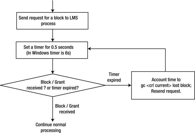
Figure 9-7. gc lost block logic
The SQL Trace file of a process stuck waiting for a block is as follows. The foreground process is waiting for a block with file#=33, block#=1701. You can see the approximate wait time of 0.5 seconds in the ela= field for these waits. After 0.5 seconds of sleep, the process re-requests for the block, but the block is not received in that interval, going into a continuous sleep-resend cycle. (In this problem scenario, due to a switch issue, few blocks were blocked by the switch never arriving to the requestor.)
*** 2012-04-05 10:51:47.280
WAIT #47390186351424: nam='gc cr block lost' ela= 520692 p1=33 p2=1701 p3=1 obj#=409860
*** 2012-04-05 10:51:48.318
WAIT #47390186351424: nam='gc cr block lost' ela= 516782 p1=33 p2=1701 p3=1 obj#=409860
WAIT #47390186351424: nam='gc cr block lost' ela= 523749 p1=33 p2=1701 p3=1 obj#=409860
...
Parameter _side_channel_batch_timeout_ms controls the duration of sleep in a database instance and defaults to 0.5 seconds (prior to 10gR2, this parameter default value was 6 seconds) in the Unix platform. On Windows, another parameter, _side_channel_batch_timeout, is used with a default value of 6 seconds. There is no reason to modify any of these parameters.
It is always important to quantify the effect of a wait event; in a perfectly healthy database, you can expect a few waits for lost block–related wait events, and you should ignore those events if the DB time spent waiting for lost blocks is negligible. Also, it is possible for another event such as gc current block receive time or gc cr block receive time to be elevated due to the loss of blocks.
Figure 9-8 shows an AWR report for the duration of a few minutes; 62% of DB time was spent in waiting for gc cr block lost event. As the percentage of DB time spent on this wait event is very high, this database must be reviewed further to identify the root cause.

Figure 9-8. Top five timed foreground events
Blocks can be lost due to numerous reasons such as network drops, latencies in CPU scheduling, incorrect network configuration, and insufficient network bandwidth. When a process is scheduled to run on a CPU, that process will drain socket buffers to application buffers. If there are delays in CPU scheduling, then the process might not be able to read socket buffers quick enough. If the incoming rate of packets to the socket buffers for that process is higher, then the kernel threads might encounter “buffer full” condition, and kernel threads will drop incoming packets silently. So, all necessary IP packets may not arrive, leading to UDP segment reassembly failures.
If there are lost block issues and if the DB time spent on lost block issue is not negligible, then you should identify if there was any CPU starvation in the server during the problem duration. I have seen severe latch contention causing higher CPU usage leading to lost block issues. Also, kernel threads have higher CPU priority than the User Foreground processes, so, even if the foreground processes are suffering from CPU starvation, kernel threads can receive the network frames from the physical link layer and fail to copy the frames to socket buffers due to “buffer full” conditions.
Network kernel parameters must be configured properly if the workload induces a higher rate of cluster interconnect traffic. For example, rmem_max and wmem_max kernel parameters (Linux) might need to be increased to reduce the probability of buffer full conditions.
Memory starvation is another issue that can trigger a slew of lost bock waits. Memory starvation can lead to swapping or paging in the server affecting the performance of foreground processes. So, foreground processes will be inefficient in draining socket buffers and might not be able to drain network buffers quick enough, leading to ”buffer full” conditions. On the Linux platform, HugePages is an important feature to implement; without HugePages configured, kernel threads can consume all available CPUs during memory starvation, thus causing the foreground process to suffer from CPU starvation and lost blocks issues.
In summary, identify if the DB time spent for lost block waits is significant. Check if the resource consumption in the database server(s) is good, verify that kernel parameters related to network are properly configured, and verify if the routes between the nodes are optimal. If resolving these problems does not resolve the root cause, then review link/switch layer statistics to verify if there are any errors.
Configuring Network for Oracle RAC and Clusterware
As we discussed at the beginning of this chapter, Oracle RAC and Oracle Grid Infrastructure require three types of network configurations: public network, private network, and storage network. The public network is primarily for the database clients to connect to the Oracle database. Also, the public network may connect the database servers with the company corporate network, through which applications and other database clients can connect to the database. The private network is the interconnect network just among the nodes on the cluster. It carries the cluster interconnect heartbeats for the Oracle Clusterware and the communication between the RAC nodes for Oracle RAC cache fusion. The storage network connects the RAC nodes with the external shared storage. This chapter focuses on public network as well as private network. Chapter 2 has more details about the configuration of the storage network. The configuration of the public and private networks consists of the following tasks:
- Configuring network hardware
- Configuring network in OS
- Establishing the IP address and name resolution
- Specifying network configuration in Grid Infrastructure installation
The next few sections discuss the configuration of these two types of network.
Network Hardware Configuration
The network hardware for Oracle RAC and Oracle Clusterware includes the NICs or network adapters inside the hosts and the network switches between the hosts (nodes) or between the host and storage. For example, each host can have multiple NICs, and some NICs can have multiple ports. Each port is presented as a network interface in OS. These network interfaces are numbered as eth0, eth1, and so on in Linux. As a minimal configuration, two network interfaces are required; one for public network and one for the private network (one NIC portis needed for the storage if you use network based storage). You should use the network switch for the network connection and should not use the crossover cable for the private interconnect to connect between the RAC nodes. For high availability, it is highly recommended that you use the following redundant configuration:
- One or two network interfaces for the public network with one or two redundant public switches to connect to the public network
- Two network interfaces for the private network with two dedicated physical switches that are connected only to the nodes on the cluster. These two network interfaces should not be on the same NIC if you use a dual-port NIC.
- Two or more network interfaces or HBAs for the storage network with two or more dedicated switches, depending on the storage network protocol.
With Oracle HAIP, you can configure up to four network interfaces for the private network. Exactly how many network interfaces you can use for each network is also limited by the total number of the NIC ports you have on your server. However, you should use the same network interface for the same network in all the nodes in the same cluster. For example, you can use eth0 and eth1 for the public network and eth3 and eth4 for the private network on all the nodes.
The network adapter for the public network must support TCP/IP protocol, and the network adapter for the private network must support the UDP. The network switch for the private network should support TCP/IP, and it should be at least 1-gigabit Ethernet or higher to meet the high-speed interconnect requirement. Recently, higher-speed networks such as 10-gigabit Ethernet or InfiniBand switches have been widely adapted for private network. To use a higher-speed network for private network, you need to make sure that all the components on the network path such as NICs, network cables, and switches, operate at higher speed.
It is important that these networks should be independent and not physically connected. It is also recommended that two dedicated switches be used for the private interconnect. Figure 9-9 shows an example of such a fully redundant private network between two nodes of the clusters.

Figure 9-9. A fully redundant private network configuration
In this example, both nodes dedicate two network ports, port 4 and port 6, to the private network. Each of these two network ports connects two different-gigabit Ethernet switches dedicated to the private network. These two switches are also interconnected with two redundant network cables, as shown in Figure 9-9. Although this example shows the private network configuration of a two-node cluster, a cluster with three or more nodes is connected in a similar way. This configuration ensures there is no single point of failure on the private network.
Once you decide the network interfaces for the public network and private network, you can start configuring these two networks based on the network interfaces. In this chapter, we mainly focus on how to configure network in Linux.
The public network includes the network interface and the IP address of the host and virtual hostname/IP for each node and the SCAN name/IP for the cluster. Configuring the public network requires you to do the following:
- Give the hostname and its IP address of each RAC node. For example, you have two hosts and their IP addresses: k2r720n1(172.16.9.71) and k2r720n2 (172.16.9.72). Be aware that the hostname should be composed of alphanumeric characters, and the underscore (“_”) is not allowed in the hostname.
- Configure the network interface of the public network on each RAC node. For example, on Linux, edit /etc/sysconfig/network-scripts/ifcfg-eth0:
DEVICE=eth0
BOOTPROTO=static
HWADDR=00:22:19:D1:DA:5C
ONBOOT=yes
IPADDR=172.16.9.71
NETMASK=255.255.0.0
TYPE=Ethernet
GATEWAY=172.16.0.1
In the preceding output, 172.16.9.71 is the IP address of the public network for the node.
- Assign the virtual hostname and VIP for each RAC node. It is recommended that you use the format <public hostname>-vip for the virtual hostname, for example, racnode1-vip. An example we have set for the following virtual names and VIPs for test cluster: k2r720n1-vip with IP address 172.16.9.171 and k2r720n2-vip with IP address 172.16.9.172
- Give the SCAN (Single Client Access Name) and three SCAN VIPs for the Cluster.For example, we have set the SCAN name kr720n-scan with three scan IP: 172.16.9.74, 172.16.9.75, 172.16.9.76.
- To achieve the high availability and load balancing, multiple redundant network interfaces for the private network should be bonded or teamed together with OS bonding or teaming methods prior to 11gR2 (11.2.0.2). With the introduction of Oracle HAIP in 11.2.0.2, bonding or teaming in OS is no longer needed, as HAIP allows you to use these redundant network interfaces directly for the private interconnect, and HAIP handles the load balance across these network interfaces and the failover to other available network interfaces in case any of these network interfaces is not responding. The following shows the example of the two network interfaces, eth1 and eth2:
DEVICE=eth1
HWADDR=BC:30:5B:ED:68:C1
ONBOOT=yes
BOOTPROTO=static
TYPE=Ethernet
IPADDR=192.168.9.71
NETMASK=255.255.255.0

DEVICE=eth2
HWADDR=BC:30:5B:ED:68:C2
ONBOOT=yes
BOOTPROTO=static
TYPE=Ethernet
IPADDR=192.168.9.72
NETMASK=255.255.255.0
After you complete the configuration and save the files, you can restart the network service:
#Service network restart
Then you can use these two network interfaces, eth12 and eth2, directly for the private network configuration during the Oracle Grid Infrastructure installation.
Establishing IP Address and Name Resolution
As you connect to a host using the hostname, Oracle database clients connect to the database using a SCAN name. These hostnames and SCAN names need to be resolved into their associated IP addresses to allow the clients to connect. In Oracle RAC and Clusterware, the SCAN name can be resolved into up to three SCAN IPs. For example, the SCAN name kr720n-scan are resolved into three IPs, 172.16.9.74, 172.16.9.75, and 172.16.9.76, in the following example. The virtual hostname is resolved into the VIP; for example, k2r720n1-vip being resolved to VIP 172.16.9.171. The public hostname is resolved into the host IP; for example, k2r720n1 being resolved into 172.16.9.71.
The technology to resolve a name to the IP address is called name resolution. In the Oracle RAC environment, there are two ways to implement this name resolution: 1) name resolution using DNS, and 2) name resolution using GNS (Grid Naming Services). Oracle recommends that you establish a static hostname resolution using DNS for all non-VIP node public hostnames. You can use either DNS or GNS for the VIP name resolution. In the following sections, we will use two clusters as an example to show the configuration of each of these two methods and how it works: 1) kr720n-cluster for the DNS method, and 2) owirac-cluster for the GNS method.
In the DNS method, you need to register the SCAN name of the cluster and the virtual hostnames and public hostname of each cluster node along with the corresponding IP address. This registration is performed on the DNS server as well as on the DNS clients which are all the cluster nodes.
On the DNS server, we need to add the name resolutions for the SCAN name, virtual hostname(VIP), and public hostname on DNS. The following example shows the added entries in the DNS for the “kr720n-cluster” cluster:
       kr720n-scan.dblab.com    IN   A  172.16.9.74
                                IN   A  172.16.9.75
                                IN   A  172.16.9.76
       k2r720n1.dblab.com       IN   A  172.16.9.71
       k2r720n1-vip.dblab.com   IN   A  172.16.9.171
       k2r720n2.dblab.com       IN   A  172.16.9.72
       k2r720n2-vip.dblab.com   IN   A  172.16.9.172
On each DNS client that is a node in the cluster, we need to configure the /etc/resolve.conf file by adding the entries that resolve the DNS server.
#cat /etc/resolv.conf
search dns.dblab.com
nameserver 172.16.150.55
Here, dns.dblab.com is the DNS server hostname, and 172.16.150.55 is the DNS server IP address on the network.
On each RAC node, you also need to modify /etc/nsswitch.conf file to change the entry
        hosts:   files  nis  dns
To
        Hosts:   dns files  nis
After saving the change on /etc/nsswitch.conf, you need to restart the nscd daemon on each node with the following command:nscd daemon on each node with the following command:
#/sbin service restart
This method places the DNS entry first and the NIS entry at the end of the search.
Oracle also recommends that you add the public hostnames and IP addresses of all the nodes on /etc/hosts file on the each node. For example, add these two entries in /etc/hosts on each node.
#public
172.16.9.71  k2r720n1.dblab.com k2r720n1
172.16.9.72  k2r720n2.dblab.com k2r720n2
It is also recommended that you do not add the SCAN name and IPs in the /etc/hosts file. Let DNS resolve SCAN VIPs.
After this configuration is completed, you can ping the SCAN name and each host’s virtual hostname. The DNS resolves the names to IPs; however, these IPs are not started until you finish the Grid Infrastructure installation using these names and VIPs and start the Grid Infrastructure. All the VIP addresses, including SCAN VIP addresses, should not be used for other purposes and should not be ping-able before the Grid Infrastructure installation completes.
As remarked previously, in this DNS method you need to add three entries for the SCAN; one entry each for the virtual hostname for every node in the cluster; and one entry each for the public hostname for every node on the cluster. This manual configuration is not too cumbersome for a small environment; however, in a production environment with many RAC clusters, each cluster with many nodes, numerous DNS entries must be configured. For example, a six-node cluster requires 2 x 6 + 3 = 15 entries, and ten such clusters require 150 entries. As the number of cluster databases and the total number of nodes increase, the DNS methods became less manageable. For this reason, Oracle 11gR2 Clusterware introduced the second method called GNS.
GNS provides name resolution for VIPs based on DHCP (Dynamic Host Configuration Protocol). In this method, GNS provides dynamic IP addresses for the virtual hostnames of all the nodes and SCAN in the cluster, through the DHCP service. In GNS, the only GNS VIP is given a static IP, and this static GNS VIP is registered in DNS. The GNS method use the subdomain delegation, DNS forwards any network name request on a particular subdomain to the GNS server, and the GNS will provide the name resolution to the dynamic IP. GNS uses multicast Domain Name Server (mDNS) in the Oracle Clusterware to provide a DHCP IP address mapping to the VIP name. The benefit of GNS is the simplification of SCAN VIPs and node VIPs by moving the management of these VIPs from DNS to the GNS local to the cluster. With GNS, adding or deleting a node is even simpler than with the DNS method, as there is no change in DNS when you add or delete a node.
Here, we use the knewrac cluster as an example to illustrate how GNS name resolution works (Figure 9-10) and the steps to configure it.

Figure 9-10. Name resolution using GNS
This cluster uses the subdomain kcloud.dblab.com. In DNS, two entries are requested:
the static IP address of GNS VIP: 172.16.15.9
the subdomain deligagtion:
subdomainkcloud.dblab.comto GNS server gns.kcloud.dblab.com
With the proceeding setup, any host request in the domain “*.kblod.dblab.com”, for example, knewrac-scan.kclod.dblab.com, will be handed off to the GNS server: gns.kcloud.dblab.com with VIP address 172.16.15.9. This GNS server maps the VIP name knhewrac-scan.kclod.dblab.com to one of the three SCAN VIPs: 172.16.150.40, 172.16.150.83, or 172.16.150.28.
The steps for implementing GNS name resolution using this example are as follows:
Step 1: On the DNS server, add a zone dblab.com to /etc/named.conf file. This zone handles DNS queries for the domain’s subnet, “dblab.com”:
zone "dblab.com" {
type master;
file "dblab.com.zone";
};
Then, add these entries to the zone file /var/named/dblab.com.zone to specify the VIP of GNS server gns.kcloud.dblab.com: 172.16.150.9 and the subdomain kcloud.dblab.com delegation to forward to GNS server gns.kcloud.dblab.com.
# cat/var/named/dblab.com.zone
       。。。。。。
$ORIGIN kcloud.dblab.com.
@       IN      NS     gns.kcloud.dblab.com.
gns.kcloud.dblab.com.    IN      A      172.16.150.9
Step 2: On all DNS clients (all the nodes in the cluster), add these entries to /etc/resolve.conf file:
# cat /etc/resolv.conf
options attempts: 2
Options timeout: 1
nameserver 172.16.15.9
nameserver 172.16.168.8
searchkcloud.dblab.com dblab.com
Here, 172.16.168.8 is the IP of the DNS server and 172.16.15.9 is the GNS server VIP of the cluster.
Step 3: Enable the “Configure GNS” option in Grid Infrastructure installation and specify the GNS configuration, including GNS subdomain and GNS VIP address. The Grid Infrastructure installation will create and configure GNS service. This will be discussed in the next session.
Network Specification in Grid Infrastructure Installation
With all the configurations and preparation work done, you can complete the network configuration through Oracle Grid Infrastructure installation. During the installation, the network configuration information, such as the public hostname and virtual hostname of each node in the cluster, the SCAN name, and the network interfaces for the public and private networks, have to be specified.
Select Whether or Not to Use GNS
If you decide to use GNS for the name resolution, you need to check the box next to “Configure GNS” on the Grid Plug and Play information page. In Oracle 12c, a single GNS can be shared by multiple clusters. When you create a new cluster, you can either share an existing GNS with other cluster by selecting “Use Shared GNS” or create a new GNS by selecting the “Create a New GNS” option. On the same page, you also need to fill out the GNS subdomain and the GNS VIP address as shown in Figure 9-11, which uses the knewrac cluster as an example.

Figure 9-11. Specifying the GNS configuration
If you use the typical standard cluster installation, in which you by default use the DNS, you leave the “Configure GNS” box unchecked. However, if you plan to implement the Oracle Flex Cluster option in Oracle 12cR1, you are required to configure GNS with a fixed VIP on one of the hub nodes.
Refer to Chapter 4 for a detailed discussion of the network configuration for Flex Clusters and Flex ASM.
At that point, the public hostname and virtual hostname of all the nodes in the cluster will be specified, as shown in the following knewrac cluster installation (Figure 9-12).

Figure 9-12. Specifying public hostnames and virtual hostnames
During the Flex Cluster installation, you need to specify the role of each node: hub node or leaf node.
The network interfaces for public and private networks also need to be specified. Since Oracle introduced HAIP in 11.2.0.2, we can directly use multiple network interfaces (NICs) for the private interconnect configuration. Figure 9-13 shows an example of selecting two network interfaces, eth1 and eth2, for the private interconnect network.

Figure 9-13. Specifying network interfaces
If you plan to use Oracle 12c Flex ASM, you need to specify the network interface for ASM network, which allows ASM clients to connect with the remote ASM instances. In Oracle 12cR1, you can have ASM network and Private network share the same network interfaces. Figure 9-13 shows that the ASM network and the private network share the same network interfaces, eth1 and eth2.
After a successful installation of the Grid Infrastructure, you can verify the network configuration.
On the knewrac cluster, the SCAN name with the VIPs dynamically generated by DHCP are as follows:
$ srvctl config scan
SCAN name:knewrac-scan.kcloud.dblab.com, Network: 1
Subnet IPv4: 172.16.0.0/255.255.0.0/eth0
Subnet IPv6:
SCAN 0 IPv4 VIP: -/scan1-vip/172.16.150.40
SCAN name: knewrac-scan.kcloud.dblab.com , Network: 1
Subnet IPv4: 172.16.0.0/255.255.0.0/eth0
Subnet IPv6:
SCAN 1 IPv4 VIP: -/scan2-vip/172.16.150.83
SCAN name: knewrac-scan.kcloud.dblab.com, Network: 1
Subnet IPv4: 172.16.0.0/255.255.0.0/eth0
Subnet IPv6:
SCAN 2 IPv4 VIP: -/scan3-vip/172.16.150.28
Notice that Oracle 12cR1 adds support for the IPv6 protocol for network configuration.
The VIPs for the public hosts on owirac-cluster cluster are as follows:
$ srvctl config vip -n knewracn1
VIP exists: network number 1, hosting node knewracn1
VIP IPv4 Address: -/knewracn1-vip/172.16.150.37
VIP IPv6 Address:

$ srvctl config vip -n knewracn2
VIP exists: network number 1, hosting node knewracn2
VIP IPv4 Address: -/knewracn2-vip/172.16.150.182
VIP IPv6 Address:
Network Configuration in Clusterware
Network configuration is stored in OCR, and Clusterware manages the network using the configuration stored in the Clusterware. Configuration details about both public and private networks are stored in the form of resources in Clusterware. Clusterware monitors network interfaces for high availability reasons.
VIP addresses and listeners are configured in a public network. Three types of Clusterware resources with dependency between them are configured to track the network and its status. Figure 9-14 shows three types of resources implementing public network.

Figure 9-14. Public network resources
A Clusterware resource of type ora.network.type is created for each subnet. First, network resource is created with a cardinality of 1 and named ora.net1.network resource. The output of the following crsctl command shows a resource created for the public network. This network is owned by the root user, with oracrs userid having Read and Execute permissions.
$ crsctl stat res ora.net1.network -p |more
NAME=ora.net1.network
TYPE=ora.network.type
ACL=owner:root:rwx,pgrp:root:r-x,other::r--,group:oinstall:r-x,user:oracrs:r-x
...
The resource attribute agent_filename indicates that this resource is monitored by orarootagent process. Also, if there are errors, then the resource is restarted five times before the resource is marked offline.
AGENT_FILENAME=%CRS_HOME%/bin/orarootagent%CRS_EXE_SUFFIX%
...
RESTART_ATTEMPTS=5
SCRIPT_TIMEOUT=60
Interfaces eth1 and eth2 are configured for the public network. Further, this resource captures subnet details of the public network; thus, all IP public addresses must be in this configured subnet.
...
USR_ORA_IF=eth1 eth2
USR_ORA_NETMASK=255.255.254.0
USR_ORA_SUBNET=10.11.45.0
VERSION=12.1.0.0.0
Network configuration as discussed so far can also be easily retrieved using the srvctl command. Output of the srvctl command shows that there is a net1 network configured in the 10.11.45.0 subnet on the eth1 and eth2 interfaces.
$ srvctl config network
Network exists: 1/10.11.45.0/255.255.254.0/eth1:eth2, type static
The VIP address is configured as a dependent resource of the ora.net1.network resource in Clusterware. The VIP resource is named ora.<node name>.vip; in this example configuration, the name of the resource is ora.rac1.vip. If the network is restarted, then the VIP resource is also restarted by the dependency-tracking mechanism. Note that the type of VIP resource is ora.cluster_vip_net1.type, and this type will be used to build dependency in listener resources.
$ crsctl stat res ora.rac1.vip -p
NAME=ora.rac1.vip
TYPE=ora.cluster_vip_net1.type
...
DESCRIPTION=Oracle VIP resource
ENABLED=1
...
START_DEPENDENCIES=hard(ora.net1.network) pullup(ora.net1.network)
STOP_DEPENDENCIES=hard(ora.net1.network)
The VIP address rac1-vip is associated with this resource. The IP address of this VIP is queried from DNS or /etc/hosts file, and that IP address must be in the same subnet as the subnet of dependent network resource (in this example, 10.11.45.0).
...
USR_ORA_ENV=
USR_ORA_VIP=rac1-vip
VERSION=12.1.0.0.0
You can also query VIP configuration using the srvctl command.
$ srvctl config vip  -n rac1
VIP exists: /rac1-vip/10.11.45.35/10.11.45.0/255.255.254.0/eth1:eth2, hosting node rac1
Listener is configured as a dependent resource of the VIP resource. The owner of Grid Infrastructure will be the owner of this resource.
$ crsctl stat res ora.LISTENER.lsnr -p

NAME=ora.LISTENER.lsnr
TYPE=ora.listener.type
ACL=owner:oracrs:rwx,pgrp:oinstall:rwx,other::r--
...
AGENT_FILENAME=%CRS_HOME%/bin/oraagent%CRS_EXE_SUFFIX%
...
Listener resource will be checked every 60 seconds, and the check command should complete in 30 seconds. Also, the port number of the listener is configured in the ENDPOINTS field of this resource. Listener resource is a dependent resource of type ora.cluster_vip_net1.type. As discussed earlier in this section, VIP resource is of type ora.cluster_vip_net1.type. Startup or shutdown of any resource with ora.cluster_vip_net1.type will trigger the listener resource to be restarted.
CHECK_INTERVAL=60
CHECK_TIMEOUT=30
...
ENDPOINTS=
...
ORACLE_HOME=%CRS_HOME%
PORT=1521
...
START_DEPENDENCIES=hard(type:ora.cluster_vip_net1.type) pullup(type:ora.cluster_vip_net1.type)
START_TIMEOUT=180
STATE_CHANGE_TEMPLATE=
STOP_DEPENDENCIES=hard(intermediate:type:ora.cluster_vip_net1.type)
...
USR_ORA_ENV=ORACLE_BASE=/opt/app/rac/crsbase
You can also query listener configuration using srvctl command. The listener is listening on port 1521 using TCP protocol.
$ srvctl config listener -l LISTENER
Name: LISTENER
Network: 1, Owner: oracrs
Home: <CRS home>
End points: TCP:1521In version 11gR2 and prior, VIP and SCAN IP addresses must be static IP addresses, meaning that VIP/SCAN/Public DNS alias to IP address mapping is statically stored in a DNS server. Version 12c supports DHCP-generated IP addresses for public, VIP and SCAN IP addresses. In version 12c, during cluster startup, DNS is queried by a VIP agent to identify IP addresses associated with DNS aliases, and retrieved IP addresses are used to configure VIP and SCAN resources. We recommend using static IP addresses for public, VIP, and SCAN IP address unless there is a valid reason to use DHCP-generated IP addresses. In environments with numerous RAC clusters, the use of GNS may be a preferred option.
In summary, the resource ora.net1.network captures the subnet and netmask details; resource ora.rac1.vip captures the VIP address and is dependent upon ora.net1.network resource; and ora.LISTENER.lsnr captures the protocol and port number details and is dependent upon ora.rac1.vip type. Any change in a resource will trigger dependent resources to be restarted or stopped.
The SCAN VIP and SCAN listener configuration is also stored as resources in Clusterware. SCAN listener simply acts as a redirection mechanism for a new connection, and VIP listeners do the heavy lifting of connection creation. (Further details about SCAN listener are given in Chapter 3, as part of the workload management discussion). The following crsctl command shows that the ora.scan1.vip resource is dependent on the ora.net1.network resource.
$ crsctl stat res ora.scan1.vip -p |more
NAME=ora.scan1.vip
TYPE=ora.scan_vip.type
ACL=owner:root:rwx,pgrp:root:r-x,other::r--,group:oinstall:r-x,user:oracrs:r-x
CARDINALITY=1
...
SCAN_NAME=rac1-scan
SCRIPT_TIMEOUT=60
START_DEPENDENCIES=hard(ora.net1.network) dispersion:active(type:ora.scan_vip.type) pullup(global:ora.net1.network)
...
STOP_DEPENDENCIES=hard(ora.net1.network)
...
USR_ORA_VIP=10.11.45.99
VERSION=12.1.0.0.0
As the subnet value is coded in the ora.net1.network resource, SCAN VIP also should be in the same subnet as other VIP resources. All VIPs and SCAN VIPs of a network should be configured in the same subnet. You can query the SCAN details using the following srvctl command. By specifying an ordinal number with –i flag, command output is filtered to just the SCAN1 resource.
$ srvctl config scan -i 1
SCAN name: rac1-scan, Network: 1/10.11.45.0/255.255.254.0/eth1:eth2
SCAN VIP name: scan1, IP: /rac-scan.local.net/10.11.45.99
Similarly, SCAN listener is configured as a resource specifying port number and protocol. SCAN listener is a dependent resource of ora.scan1.vip.
$ crsctl stat res ora.LISTENER_SCAN1.lsnr -p  |more
NAME=ora.LISTENER_SCAN1.lsnr
TYPE=ora.scan_listener.type
...
PORT=25000
...
START_DEPENDENCIES=hard(ora.scan1.vip) dispersion:active(type:ora.scan_listener.type) pullup(ora.scan1.vip)
...
STOP_DEPENDENCIES=hard(intermediate:ora.scan1.vip)
Up to version 11gR2, SCAN IP addresses were required to be in the first network only. Version 12c allows you to create SCAN listeners and SCAN IP addresses in the second network also.
In summary, the resource ora.net1.network captures the subnet and netmask details; resource ora.scan1.vip captures the VIP address and is dependent on ora.net1.network resource; and ora.LISTENER_SCAN1.lsnr captures the protocol and port number details, and is dependent on ora.scan1.vip type. Any state change in a resource will trigger dependent resources to be restarted or stopped.
Private network configuration is also stored in OCR, and OCR can be stored in ASM from Database version 11g onward. However, during Clusterware startup, the CSSD daemon is started earlier than the ASM instance. So, a few critical details are required for HAS startup and are captured in an XML file and Oracle Local Registry (OLR). The following lines show cluster_interconnect details in the profile.xml file.
$ cd $ORACLE_HOME/gpnp/profiles/peer/
$ grep 172 profile.xml
...
<gpnp:Network id="net3" IP="172.18.1.0" Adapter="eth3" Use="cluster_interconnect"/>
<gpnp:Network id="net4" IP="172.18.2.0" Adapter="eth4" Use="cluster_interconnect"/>
...
A Clusterware resource is employed to monitor the private network with the HAIP feature. The resource ora.cluster_interconnect.haip implements the HAIP feature for cluster interconnect, and an oraroot agent monitors these private network interfaces.
$ crsctl stat res ora.cluster_interconnect.haip -init  -p |more
NAME=ora.cluster_interconnect.haip
...
START_DEPENDENCIES=hard(ora.gpnpd,ora.cssd)pullup(ora.cssd)
START_TIMEOUT=60
STATE_CHANGE_TEMPLATE=
STOP_DEPENDENCIES=hard(ora.cssd)
...
USR_ORA_IF_GROUP=cluster_interconnect
Resource ora.cluster_interconnect.haip is also dependent upon CSSD and GPNP resource. So, this resource is started after CSSD startup. Also, notice that USE_ORA_IF_GROUP is specified as cluster_interconnect, referring to the network interface details stored in the GPNP profile.
The following output is taken from orarootagent_root log files. As you see in the following, the HAIP resource is configuring link local IP addresses on the interfaces designated for cluster_interconnect. The agent monitors these network interfaces too. If any interface fails, then the link local IP addresses are reconfigured to an available interface, thus providing high availability.
[ USRTHRD][16] {0:0:2} HAIP: initializing to 2 interfaces
[ USRTHRD][16] {0:0:2} HAIP: configured to use 2 interfaces
[ USRTHRD][16] {0:0:2} HAIP: Updating member info HAIP1;172.18.1.0#0
[ USRTHRD][16] {0:0:2} InitializeHaIps[ 0] infList 'inf eth3, ip 172.18.1.0, sub 172.18.1.0'
[ USRTHRD][16] {0:0:2} HAIP: starting inf 'eth3', suggestedIp '169.254.28.111’, assignedIp ''
[ USRTHRD][16] {0:0:2} Thread:[NetHAWork]start {
[ USRTHRD][16] {0:0:2} Thread:[NetHAWork]start }
[ USRTHRD][17] {0:0:2} [NetHAWork] thread started
[ USRTHRD][16] {0:0:2} HAIP: starting inf 'eth4', suggestedIp '169.254.78.111', assignedIp ''
Prior to 11g, private network details were stored in OCR only. Changing the private network details was easier. From 11g onward, since private network configuration is stored in OCR, OLR, and profile.xml file, you need to pay special attention to the sequence of steps to modify the private network configuration. Incorrect sequencing of steps will lead to hung Clusterware startup. The high-level sequence of steps is as follows: 1) add private network interface using oifcfg add if command, 2) shut down the Clusterware, 3) change the interface details in the database node, 4) restart Clusterware, and then 5) delete old private network details. As the oifcfg command updates the profile.xml file and OLR, change using oifcfg command is the correct way to modify network configuration. If you have modified the private network in the OS without modifying the Clusterware, then a special procedure is needed to update the profile.xml file. Profile.xml files are signed XML files; you should not update profile.xml file directly either.
Database instance and ASM instance query Clusterware to identify the private network details and use that configuration for private network traffic. For example, the gv$cluster_interconnects view shows the interface and IP address used for private interconnect traffic. Notice that the SOURCE column is null, indicating that this is queried from Clusterware processes.
RS@SQL> select * from gv$cluster_interconnects order by inst_id;

INST_ID NAME          IP_ADDRESS          IS_ SOURCE
---------- --------------  ----------------          --- ------------------------------
             1 ce0:1           169.254.72.158     NO
             1 ce6:1           169.254.195.203    NO
             2 ce6:2           169.254.60.160     NO
             2 ce6:1           169.254.181.11     NO
You can also use specific IP addresses using the cluster_interconnnects initialization parameter. Usually, changes to the cluster_interconnects parameter are not needed, as the database will retrieve link local IP addresses from the Clusterware processes, so this parameter is best left untouched from 11gR2 onward. Notice that the SOURCE column indicates the source of the IP address values; in this example, values are retrieved from the cluster_interconnects database parameter.
cluster_interconnects                string      172.29.1.11:172.29.2.12

RS @ RAC1> select * from gv$cluster_interconnects
INST_ID NAME            IP_ADDRESS       IS_ SOURCE
---------- --------------- ---------------- --- -------------------------------
         1 aggr3           172.29.1.11      NO  cluster_interconnects parameter
         1 aggr4           172.29.2.12      NO  cluster_interconnects parameter
         3 aggr3           172.29.1.31      NO  cluster_interconnects parameter
         3 aggr4           172.29.2.32      NO  cluster_interconnects parameter
         2 aggr3           172.29.1.21      NO  cluster_interconnects parameter
         2 aggr4           172.29.2.22      NO  cluster_interconnects parameter
Network failover can happen in both public and private network interfaces. As Clusterware processes are monitoring network interfaces, failure is immediately detected, and appropriate action is taken to improve high availability.
If there is OS-based network high availability solution already configured, such as Linux Bonding, then the high availability is handled completely by the OS solution. Clusterware does not implement high availability solution in this scenario and simply uses the implemented OS solution.
If there is no OS-based solution, then HAIP can be used for cluster interconnect to implement high availability. If the private network interface fails, and if there are multiple interfaces configured for cluster interconnect, then the link local IP address from the failed interface is failed over to the available interface. Database connections might briefly run into errors during the IP reconfiguration, but those errors should quickly disappear, and in most cases, foreground processes will retry a request and succeed. After a link local IP failover to a surviving interface, Clusterware will perform re-ARP inducing a new map between an IP address and MAC address.
If all interfaces configured for cluster interconnect fail, then the link local address cannot be configured in any interface. This would also lead to heartbeat failure; so, rebootless restart or node eviction might be the result.
If a network adapter for public network fails, and if there are no other suitable adapters configured, then the VIP listener will be shut down, and VIP address will fail over to a surviving node, but no listener will be restarted on failed-over VIP. Any new connection to that failed VIP will get CONN RESET immediately, and the connection will try the next connection entry in the list.
If a network adapter for SCAN IP fails, then the SCAN IP and SCAN listener will be failed over to a surviving node.
In 11gR2, you can configure second network for public VIPs only. However, the second network cannot be configured for cluster interconnect or SCAN network. In version 12c, the second network is supported for public, VIP, and SCAN IP addresses. Second network is useful if there are multiple subnets configured for public network traffic to the database.
The first step in adding second network resources is to add a network resource. The following command uses –k 2, indicating that this is a second network, and lists the subnet as 10.5.12.0 on aggr1 and aggr2 devices.
$ srvctl add network –k 2 –S 10.5.12.0/255.255.254.0/aggr1:aggr2
Next, the VIP on that network is added using the following srvctl commands. For all commands, -k 2 indicates that this VIP is for second network. A listener listening on second network port 1521 is also added using the add listener command.
$ srvctl add vip –n node1 –k 2 -A 10.5.12.99/255.255.254.0/aggr1:aggr2
$ srvctl add vip –n node2 –k 2 -A 10.5.12.100/255.255.254.0/aggr1:aggr2
$ srvctl add listener –l listener2 –p 1521 –k 2
The next command modifies a listener_networks parameter in the database. Database PMON or LREG process registers with the listener using this configuration. Note that for the first network, SCAN listener is specified as remote_listener, but for the second network a VIP listener in remote node is specified.
alter system set LISTENER_NETWORKS='((NAME=network1)(LOCAL_LISTENER=listener_net1)(REMOTE_LISTENER=racscan:1521))','((NAME=network2)(LOCAL_LISTENER=listener_net2) (REMOTE_LISTENER=remote_net2))';
In 11gR2, while the listener_networks can be used for automatic service registration with both local VIP listener and SCAN listener, it is not possible to use SCAN listener to redirect the connection for the second network. So, the second network cannot be used in conjunction with SCAN listener as of 11gR2. Version 12c allows SCAN listeners in the second network with a seamless network management of packets staying in the same subnet. Refer to Chapter 3 for exact commands to create a SCAN listener in the second network.
Further, listeners specified in the listener_networks parameter should not be specified in local_listener or remote_listener parameter, since that will lead to cross-registration between two networks.
Summary
The network is a critical piece of RAC infrastructure. Understanding network architecture, Clusterware implementation of the network, and the performance statistics of the network is of paramount importance when designing a RAC infrastructure or debugging RAC performance issues.
Pay close attention to the kernel parameters, subnet masks, network interface configuration, etc., while configuring clusters for RAC installation. It is much easier to resolve OS errors before configuring RAC. After the RAC configuration, OS level change requires further considerations.
If you have errors in the database due to lost packets or performance issues indicating network issues, then you should review network performance metrics using OS tools to identify any network configuration or performance issues. We discussed various tools such as ping, netstat, traceroute, etc., which are essential to identify the root cause of a performance issue.
1 Node reboots can be time-consuming and Clusterware tries to avoid them by restarting itself. Of course, a Clusterware restart will cause databases and listeners to restart.
2 Softirq is an interrupt request to a CPU and it is a software-initiated interrupt request. Hardware irq is initiated by hardware. In layman’s terms, softirq is equivalent to adding a request to a CPU queue. After the end of current timeslice, a softirq is serviced by the CPU.
3 This discussion is provided to understand basics about network function calls and should not interpreted as an actual algorithm. For that matter, every kernel behaves differently.
4 Other protocols may be in use in a third-party cluster. For example, a RAC database uses LLT protocol in a Veritas SFRAC cluster.
5 IP address 8.8.8.8 is assigned to Google, and it is the IP address of Google’s public DNS server. (In numerology, number 8888 means that there is light at the end of tunnel!)
6 Release 12c allows us to use DHCP-generated IP addresses for VIPs. Discussion in this section applies to DHCP-generated IP addresses also. The only difference between static IP allocation and DHCP-generated IP allocation is that DNS server is queried to retrieve IP address associated with the DHCP aliases, at the time of cluster startup.
7 The example of home networks will help to clear up any confusion about private networks. Network Address Translation (NAT) plays a critical role in accessing public IP addresses from private IP address spaces. For example, a home network router creates a private address space. Even though home routers will usually have just one public IP address, many computers are connected to that router, and many computers can access external websites through the router.The router will translate private IP address to a port and modify return address as the public address of the router. Using the router translation table, return packets are delivered to the correct port and hence the correct computer.
8 Not all buffers are copied to buffer cache. For example, parallel query copies buffers to its PGA.
9 Version 12c introduces a new feature, HAVIP, and you should not confuse HAVIP with the HAIP feature. The HAVIP feature is applicable to public network, and the HAIP feature is applicable to private network.
10 Note that this is not a complete set of steps to create NFS exported file system.