
![]()
The Runtime Engine
Chapter 3 focused on the plans that the CBO made. It is now time to look at how those plans work out in practice. I will explain the traditional ways of gathering and analyzing runtime data as well as a newer complementary approach called the SQL performance monitor. To fully understand SQL performance, it is very important to understand the role of workareas and the shortcuts the runtime engine uses to minimize overhead, and both of these topics are covered in this chapter.
Collecting Operation Level Runtime Data
As you’ll learn in Chapter 5, we almost always need to get a breakdown of the behavior of an SQL statement at the operation level to determine how best to optimize that SQL statement. Some of the operation-level statistics that can be gathered are:
- How many times the operation ran in the course of the statement
- How long it took
- How many disk operations it performed
- How many logical reads it made
- Whether or not the operation executed entirely in memory
These statistics are not gathered by default. There are three ways to trigger the collection:
- Add theGATHER_PLAN_STATISTICSoptimizer hint to your SQL statement: The collection will be done for that one statement only.
- Change the initialization parameterSTATISTICS_LEVEL to ALL: If set at the session level, all SQL statements for the session will be affected. If STATISTICS_LEVEL is set to ALL at the system level, collection will be enabled for all SQL statements in all sessions in the instance.
- Enable SQL tracing: As with the STATISTICS_LEVEL parameter, SQL tracing can be enabled either at the session or system level.
Let’s look at each of these options in turn.
The GATHER_PLAN_STATISTICS Hint
This optimizer hint has been around for a long time but is documented for the first time in Oracle Database 12cR1. Listing 4-1 updates Listing 3-2 by adding the GATHER_PLAN_STATISTICS hint.
Listing 4-1. Gathering operation data at the statement level
SELECT /*+ gather_plan_statistics */
       'Count of sales: ' || COUNT (*) cnt
  FROM sh.sales s JOIN sh.customers c USING (cust_id)
 WHERE cust_last_name = 'Ruddy';
Notice that, as with all optimizer hints, you can use uppercase or lowercase.
Setting STATISTICS_LEVEL=ALL
If you can’t, or would prefer not to, change the code you are analyzing, you can set the STATISTICS_LEVEL parameter using one of the two statements in Listing 4-2.
Listing 4-2. Enabling runtime data collection at the session or system level
ALTER SESSION SET STATISTICS_LEVEL=ALL;
ALTER SYSTEM  SET STATISTICS_LEVEL=ALL;
Any Oracle performance specialist would be remiss not to advise you of the potential for serious performance problems when you set STATISTICS_LEVEL to ALL at the system level. The main concern is that the performance of your application could seriously degrade as a result of the additional overhead. However, many experts would go further and suggest that you should only set STATISTICS_LEVEL to ALL at the system level for short periods of troubleshooting, and that it is never appropriate to leave it set to ALL at the system level permanently. I wouldn’t go that far.
The main contributor to the overhead of gathering runtime statistics is the numerous calls to the Unix operating system routine GETTIMEOFDAY or its equivalent on other platforms. Although this operating system call can be very inefficient on some operating systems, on others it can be very efficient. In addition, the sampling frequency (controlled by the hidden parameter _rowsource_statistics_sampfreq) has been reduced in later releases of Oracle Database. I have recently set STATISTICS_LEVEL to ALL at the system level on a heavily loaded Solaris/SPARC-64 production system and found no measurable impact on the elapsed time of a two-hour batch run.
Even if you leave STATISTICS_LEVEL permanently set to ALL at a systemwide level, the runtime engine statistics are not saved in the AWR. To work around this, I run my own scheduled job to capture these data. The code for doing all of this is quite lengthy, so I haven’t included it here, but it is available in the downloaded materials.
The reason you might want to consider permanently setting STATISTICS_LEVEL to ALL at the system level is to deal with unexpected production performance problems after the event; if an SQL statement runs fine sometimes but not always, it may be that you can’t reproduce the problem at will and having the data available from the actual incident can be invaluable.
As a final note of caution, you should be aware that between versions 10.1.0.2 and 11.1.0.7 you may run into bug 8289729, which results in a dramatic increase in the size of the SYSAUX tablespace. Have a look at the Oracle support note 874518.1 or this blog from Martin Widlake (http://mwidlake.wordpress.com/2011/06/02/why-is-my-sysaux-tablespace-so-big-statistics_levelall/), but don’t be too disheartened as this extra data collection didn’t harm performance in my case.
Enabling SQL Tracing
There are several ways to enable SQL tracing. The oldest and therefore most well-known way to enable SQL tracing is to set the 10046 event. So you will often hear people refer to SQL trace as the “10046 trace.” However, the preferred way to enable SQL trace these days is to use the routine DBMS_MONITOR.SESSION_TRACE_ENABLE, and examples of how to call it are provided in the PL/SQL packages and types reference manual. Additional information can be found in the performance tuning guide (pre-12cr1) or the SQL tuning guide (12cR1 onward).
Apart from enabling statistics gathering from the runtime engine, SQL trace generates a text file with a lot of additional information about what is happening in the session. Among other things, this trace file can help you see:
- What SQL statements have run and how often they run.
- What recursive SQL statements (SQL statements in triggers or functions) have run.
- How much time was spent opening the cursor (executing the SQL statement), how much time was spent fetching the data from the cursor, and how much time was spent in so-called idle wait events, implying that the session is executing application logic outside of the database.
- Detailed information about individual wait events, such as the precise number of blocks read by individual database file multiblock read waits.
Although for many performance specialists the SQL trace is the primary diagnostic tool, I almost never use it for tuning individual SQL statements! For the vast majority of SQL tuning tasks, the runtime engine statistics are more than sufficient for the task, and as you’ll see shortly, data dictionary views are available that present those data in a very convenient way.
Displaying Operational Level Data
Once you have gathered your runtime engine statistics by one of the ways described above, the next task is to display them. Let’s look at the two ways to do this:
- With DBMS_XPLAN.DISPLAY_CURSOR
- With V$SQL_PLAN_STATISTICS_ALL
Displaying Runtime Engine Statistics with DBMS_XPLAN.DISPLAY_CURSOR
Using the nondefault parameters to DBMS_XPLAN.DISPLAY_CURSOR, you can see runtime engine statistics in the operation table. Listing 4-3 shows how to do this immediately after running the statement in Listing 4-1.
Listing 4-3. Displaying runtime engine statistics
SELECT * FROM TABLE (DBMS_XPLAN.display_cursor (format => 'ALLSTATS LAST'));

-------------------------------------------------------------------------------------
| Id  | Operation                       | Name           | Starts | E-Rows | A-Rows |
-------------------------------------------------------------------------------------
|   0 | SELECT STATEMENT                |                |      1 |        |      1 |
|   1 |  SORT AGGREGATE                 |                |      1 |      1 |      1 |
|*  2 |   HASH JOIN                     |                |      1 |   7956 |   1385 |
|*  3 |    TABLE ACCESS FULL            | CUSTOMERS      |      1 |     61 |     80 |
|   4 |    PARTITION RANGE ALL          |                |      1 |    918K|    918K|
|   5 |     BITMAP CONVERSION TO ROWIDS |                |     28 |    918K|    918K|
|   6 |      BITMAP INDEX FAST FULL SCAN| SALES_CUST_BIX |     28 |        |  35808 |
-------------------------------------------------------------------------------------
Listing 4-3 has been edited somewhat to remove various headings and some of the columns from the operation table. Once again, this is just so the output is readable on the page.
The DBMS_XPLAN.DISPLAY_CURSOR has a FORMAT parameter, and the way to get all the runtime execution statistics from the last execution of the statement is to specify the value of 'ALLSTATS LAST'; you can check the documentation for more variants. The resulting output is quite illuminating:
- First, look at the Starts column. This tells you that operations 0 through 4 ran once, but that operation 5 ran 28 times. This is because there are 28 partitions in the SALES table and it needs to run the TABLE ACCESS FULL operation for each one.
- The E-Rows and A-Rows columns are the estimated and actual row counts, respectively, and you can see that the biggest discrepancy lies with operation 2 where the estimate is over five times greater than reality.
- The actual elapsed time in column A-Time is reported with a greater degree of accuracy than the estimate displayed by DBMS_XPLAN.DISPLAY.
It is important to realize that all runtime engine statistics reflect the accumulated results of all executions of the operation. So operation 5 returned 918K rows after scanning all 28 partitions and the 0.46-second elapsed time also reflects the accumulated time to scan the entire SALES table.
ALL EXECUTIONS OF A STATEMENT VS. ALL EXECUTIONS OF AN OPERATION
I mentioned that the ALLSTATS LAST format displayed statistics for the LAST run of the SQL statement. However, I also stated that the A-Time column reflects the accumulated time from all executions of operation 5. Both statements are true because the 28 executions of operation 5 were all performed as part of the LAST execution of the SQL statement. If I had specified the ALLSTATS ALL format, then the value of Starts for operation 5 would have been a multiple of 28 if the statement had been run multiple times.
The A-Time column reflects the time taken to execute the operation and all its descendants. For example, look at the HASH join at operation 2 and its two children:
- The first child of operation 2 is the full table scan of the CUSTOMERS table at operation 3. Operation 2 is reported to have taken 0.2 second.
- The PARTITION RANGE ALL operation with ID 4 is the second child of operation 2 and apparently took 0.66 second.
- If we add 0.2 and 0.66, it totals to 0.86 second for the children of operation 2.
- Subtracting the value of 0.86 from the reported value of 1.22 in operation 2, you can see that the HASH JOIN itself took 0.36 second.
Displaying Runtime Engine Statistics with V$SQL_PLAN_STATISTICS_ALL
Although I find the output of DBMS_XPLAN functions superb when it comes to analyzing an execution plan and working out what it does, I find the format of the DBMS_XPLAN output very difficult to work with when doing detailed analysis of runtime statistics. The main problem is that there are a large number of columns, and even assuming you have an electronic page capable of displaying them all, it is difficult for the eye to navigate left and right.
The view V$SQL_PLAN_STATISTICS_ALL returns all the runtime engine statistics shown by DBMS_XPLAN.DISPLAY_CURSOR, and when I am doing any kind of detailed analysis of runtime engine data, I almost always use a tool to display the output of that view in a grid. Even if you do not have a graphical tool, such as SQL Developer, you can always get the data from the view in Comma Separated Variable (CSV) format and pop it into a spreadsheet; that works just as well.
The reason that displaying the statistics in a grid is useful is that you can order the columns as you wish and you can temporarily hide the columns you aren’t currently focused on. There are a few extra tricks you can use that can make reading these data even easier:
- V$SQL_PLAN_STATISTICS_ALL contains all of the statistics for both the last execution of a statement and all executions of the statement. The columns containing information from the last execution are prefixed with "LAST_". Because these are probably all you need, most of the time you do not want to select the columns STARTS, OUTPUT_ROWS, CR_BUFFER_GETS, CU_BUFFER_GETS, DISK_READS, DISK_WRITES, and ELAPSED_TIME because these columns reflect all executions of the statement and will cause confusion.
- You can indent the OPERATION column using the DEPTH column.
- You can label potentially ambiguous columns to avoid confusion.
- Dividing LAST_ELAPSED_TIME by 1000000 changes microseconds to seconds, more readable for most of us.
Listing 4-4 shows a simple query against V$SQL_PLAN_STATISTICS_ALL that illustrates these points.
Listing 4-4. Selecting a subset of columns from V$SQL_PLAN_STATISTICS_ALL
  SELECT DEPTH
        ,LPAD (' ', DEPTH) || operation operation
        ,options
        ,object_name
        ,time "EST TIME (Secs)"
        ,last_elapsed_time / 1000000 "ACTUAL TIME (Secs)"
        ,CARDINALITY "EST ROWS"
        ,last_output_rows "Actual Rows"
    FROM v$sql_plan_statistics_all
   WHERE sql_id = '4d133k9p6xbny' AND child_number = 0
ORDER BY id;
This query just selects a few columns, but in practice you would select a lot more. The SQL_ID and child number for the statement you are interested in can be obtained using the techniques described in Chapter 1.
Displaying Session Level Statistics with Snapper
Although the most important statistics for analysis of runtime performance are those in V$SQL_PLAN_STATISTICS_ALL, there are a plethora of statistics that are gathered constantly by default. For some unfathomable reason, Oracle has left their customers with only a bunch of impenetrable views to see these statistics, and most of us are left too disheartened to try using them. Fortunately “most” does not equal “all,” and there a number of people who have found ways to make this information easier to digest. One of the earliest examples of a script to display session statistics in a readable way came from Tom Kyte and can be found at http://asktom.oracle.com/runstats.html. In my opinion, the best tool for looking at this information comes from Oracle scientist Tanel Poder, who has published a general purpose script to extract and display numerous runtime statistics in an easily readable format. The latest version of his invaluable Snapper script is available at http://blog.tanelpoder.com/ and I encourage you to download this free and simple-to-use tool.
Snapper is particularly useful when a session is “stuck” on the CPU. On each occasion that I have used Snapper in these circumstances, I been able to see immediately what the problem was. Listing 4-5 shows a real-life extract from a Snapper run on a long-running query that was constantly on the CPU.
Listing 4-5. Contention issue highlighted by snapper
------------------------------------------------------------------------------
 TYPE, STATISTIC                                                 ,     HDELTA,
------------------------------------------------------------------------------
 STAT, session logical reads                                     ,      1.06M,
 STAT, concurrency wait time                                     ,          1,
 STAT, consistent gets                                           ,      1.06M,
 STAT, consistent gets from cache                                ,      1.06M,
 STAT, consistent gets - examination                             ,      1.06M,
 STAT, consistent changes                                        ,      1.06M,
 STAT, free buffer requested                                     ,         17,
 STAT, hot buffers moved to head of LRU                          ,         27,
 STAT, free buffer inspected                                     ,         56,
 STAT, CR blocks created                                         ,         17,
 STAT, calls to kcmgas                                           ,         17,
 STAT, data blocks consistent reads - undo records applied       ,      1.06M,
 STAT, rollbacks only - consistent read gets                     ,         17,
 TIME, DB CPU                                                    ,      5.82s,
 TIME, sql execute elapsed time                                  ,      5.71s,
 TIME, DB time                                                   ,      5.82s,
 WAIT, latch: cache buffers chains                               ,    11.36ms,
--  End of Stats snap 1, end=2013-01-31 02:29:11, seconds=10
What stood out to me when I first saw the output in Listing 4-5 was that in the 10-second snapshot it applied 1.06 million undo records! The query was in conflict with a bunch of insertion sessions that had started shortly after the query did, and the query was busy making consistent read copies by backing out the insertions. I was immediately able to see that killing and restarting the query would allow it to finish quickly. I was asked if it was necessary to gather statistics before restarting. I am able to confidently state that that wasn’t necessary. All the guesswork had been eliminated!
The statistics in V$SQL_PLAN_STATISICS_ALL have three major drawbacks:
- They are only available if you have set STATISTICS_LEVEL to ALL, which, as discussed previously, will not be problematic on some hardware platforms but may be problematic on others.
- They are only available after the statement finishes.
- The LAST statistics are missing or incorrect when parallel query operations are used.
These drawbacks make diagnosis of some problems difficult. Fortunately, SQL performance monitor was introduced in Oracle Database 11gR1 and that helps get around all of these deficiencies.
SQL performance monitor reports can be accessed either via Enterprise Manager or via a call to DBMS_SQLTUNE.REPORT_SQL_MONITOR from SQL*Plus. I’ll focus on the latter mechanism here. Listing 4-6 shows two small scripts that can be used to generate an HTML report. Personally I am not a great fan of multicolored charts when it comes to detailed analysis. Give me text output and a spreadsheet any day. However, in this case even I always generate the HTML output. Let me show you why.
You should take the first two snippets of code in Listing 4-6 and place them into two separate scripts on your PC. The third snippet shows how the scripts are called. When you call the scripts, an HTML file is produced in C:Temp, a location that is obviously changeable if you wish.
Listing 4-6. Scripts to generate an HTML report with SQL performance monitor
-- Place this code in GET_MONITOR_SID.SQL

SET ECHO OFF TERMOUT OFF LINES 32767 PAGES 0 TRIMSPOOL ON VERIFY OFF LONG 1000000 LONGC 1000000
SPOOL c:	empmonitor.html REPLACE

SELECT DBMS_SQLTUNE.report_sql_monitor (session_id => &sid, TYPE => 'ACTIVE')
  FROM DUAL;

SPOOL OFF
SET TERMOUT ON

-- Place this code in GET_MONITOR_SQLID.SQL

SET ECHO OFF TERMOUT OFF LINES 32767 PAGES 0 TRIMSPOOL ON VERIFY OFF LONG 1000000 LONGC 1000000
SPOOL c:	empmonitor.html REPLACE

SELECT DBMS_SQLTUNE.report_sql_monitor (sql_id   => '&sql_id'
                                       ,TYPE     => 'ACTIVE')
  FROM DUAL;

SPOOL OFF
SET TERMOUT ON PAGES 900 LINES 200

-- Example call to GET_MONITOR_SID.SQL from SQL*Plus

DEFINE SID=123
@GET_MONITOR_SID
Note the SQL*Plus formatting lines before the SPOOL statement. These are important to ensure the output is usable.
The next step is to place a bookmark in your browser to point to file:///c:/temp/monitor.html. You can just click this bookmark and your latest monitor report will appear!
The output contains almost all of the information that is available in V$SQL_PLAN_STATISTICS_ALL and much more besides. Figure 4-1 shows part of an SQL performance monitor report.
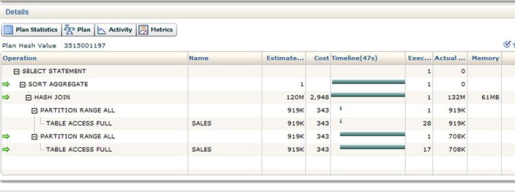
Figure 4-1. Fragment of an SQL performance monitor report
The screenshot in Figure 4-1 is from an actively running query. You see the arrows on the left? These show the operations that are currently in progress. Data are being read from the SALES table and as the rows are produced they are being matched by the HASH JOIN and then aggregated by the SORT AGGREGATE operation. Remember, the SORT AGGREGATE doesn’t sort!
The 47-second timeline in the fifth column shows that the first of the full table scans was fast but the second is running slower. You have to be careful here. The timeline figures shown by this report show when the operations first become active as well as the point when (or if) they ceased to be active; the time spent processing rows by both parent and child operations is included. Contrast this with V$SQL_PLAN_STATISTICS_ALL where the reported times include child operations but not parent ones. There is a lot of information in the SQL performance report, so play around with it.
Unfortunately, SQL performance monitor isn’t a complete replacement for V$SQL_PLAN_STATISTICS_ALL. For example, it is impossible to tell from Figure 4-1 which of the four operations currently running is taking up the time. This will only be visible once the query finishes in V$SQL_PLAN_STATISTICS_ALL. Here are a few final notes on SQL performance monitor:
- Statements are normally only monitored after they have run for more than five seconds. You can override this rule by the MONITOR and NO_MONITOR hints.
- Data from monitored SQL statements are kept in a circular buffer, so it might age out quite quickly on a busy system.
Workareas
Lots of operations in an SQL statement need some memory to function, and these allocations of memory are called workareas.
Here are some of the operations that require a workarea:
- All types of joins, with the exception of nested loops that require no workarea.
- Sorts are required, amongst other things, to implement ORDER BY clauses and by some aggregate and analytic functions.
- Although some aggregate and analytic functions require sorts, some do not. The SORT AGGREGATE operation that has come up several times in this book so far still requires a workarea, even though no sorting is involved!
- The MODEL clause requires a workarea for the cells being manipulated. This will be discussed with the MODEL clause later in this book.
Allocating Memory to a Workarea
It is the runtime engine’s job to determine how much memory to allocate to each workarea and to allocate disk space from a temporary tablespace when that allocation is insufficient. When costing operations, the CBO will hazard a guess as to how much memory the runtime engine will allocate, but the execution plan does not include any directive as to how much to allocate.
One common misconception is that memory for workareas is allocated in one big chunk. That is not the case. Workarea memory is allocated a bit at a time as it is needed, but there may come a point when the runtime engine has to declare that enough is enough and that the operation has to complete using space in a temporary tablespace.
The calculation of how much memory can be allocated to a workarea depends on whether the initialization parameter WORKAREA_SIZE_POLICY is set to MANUAL or AUTO.
Calculating Memory Allocation When WORKAREA_SIZE_POLICY Is Set to AUTO
We almost always explicitly set the initialization parameter PGA_AGGREGATE_TARGET to a nonzero value these days so automatic workarea sizing takes place. In this case, the runtime engine will try to keep the total amount of memory under the PGA_AGGREGATE_TARGET, but there are no guarantees. PGA_AGGREGATE_TARGET is used to derive values for the following hidden initialization parameters:
- _smm_max_size: The maximum size of a workarea in a statement executing serially. The value is specified in kilobytes.
- _smm_px_max_size: The maximum size of all matching workareas in a query executing in parallel. The value is specified in kilobytes.
- _pga_max_size: The maximum amount of memory that can be allocated to all workareas within a process. The value is specified in bytes.
The internal rules for calculating these hidden values seem quite complicated and vary from release to release, so I won’t try documenting them here. Just bear in mind that:
- The maximum size of any workarea is at most 1GB with automatic WORKAREA_SIZE_POLICY set to AUTO.
- The total memory for all workareas allocated to a process is at most 2GB with automatic WORKAREA_SIZE_POLICY set to MANUAL.
- Increasing the degree of parallelization for a statement will cease to have an impact on the memory available for your operation after a certain point.
Calculating Memory Allocation When WORKAREA_SIZE_POLICY Is Set to MANUAL
The only way to get individual workareas larger than 1GB or to have an SQL statement operating serially to use more than 2GB for multiple workareas is to set WORKAREA_SIZE_POLICY to MANUAL. This can be done at the session level. You can then set the following parameters at the session level:
- HASH_AREA_SIZE: The maximum size of a workarea used for HASH JOINs. This is specified in bytes and must be less than 2GB.
- SORT_AREA_SIZE: The maximum size of a workarea used for all other purposes. This includes operations such as HASH GROUP BY, so don’t get confused! The value of SORT_AREA_SIZE is specified in bytes and can be set to any value less than 2GB.
The HASH_AREA_SIZE and SORT_AREA_SIZE parameters are only used when WORKAREA_SIZE_POLICY is set to MANUAL. They are ignored otherwise.
Optimal, One-Pass, and Multipass Operations
If your sort, join, or other operation completes entirely within the memory allocated to the workarea, it is referred to as an optimal operation. If disk space is required, then it may be that the data have been written to disk once and then read back in once. In that case, it is referred to as a one-pass operation. Sometimes, if a workarea is severely undersized, data need to be read and written out more than once. This is referred to as a multipass operation. Generally, although there are some obscure anomalies, an optimal operation will complete faster than a one-pass operation and a multipass operation will take very much longer than a one-pass operation. As you might imagine, identifying multipass operations is very useful, and fortunately there are several columns in V$SQL_PLAN_STATISTICS_ALL that come to the rescue:
- LAST_EXECUTION: The value is either OPTIMAL or it specifies the precise number of passes taken by the last execution of the statement.
- ESTIMATED_OPTIMAL_SIZE: Estimated size (in kilobytes) required by this workarea to execute the operation completely in memory (optimal execution). This is either derived from optimizer statistics or from previous executions.
- ESTIMATED_ONEPASS_SIZE: This is the estimated size (in kilobytes) required by this workarea to execute the operation in a single pass. This is either derived from optimizer statistics or from previous executions.
- LAST_TEMPSEG_SIZE: Temporary segment size (in bytes) created in the last instantiation of this workarea. This column is null when LAST_EXECUTION is OPTIMAL.
Shortcuts
The runtime engine usually follows the instructions laid out by the CBO slavishly, but there are times when it uses its initiative and departs from the prescribed path in the interests of performance. Let’s look at a few examples.
Take another look at the query in Listing 3-1. Listing 4-7 executes the query and checks the runtime behavior.
Listing 4-7. An example of scalar subquery caching
SET LINES 200 PAGES 900 SERVEROUT OFF
COLUMN PLAN_TABLE_OUTPUT FORMAT a200

SELECT e.*
      ,d.dname
      ,d.loc
      , (SELECT COUNT (*)
           FROM scott.emp i
          WHERE i.deptno = e.deptno)
          dept_count  FROM scott.emp e, scott.dept d
 WHERE e.deptno = d.deptno;

SELECT * FROM TABLE (DBMS_XPLAN.display_cursor (format => 'ALLSTATS LAST'));

--------------------------------------------------------------
| Id  | Operation          | Name | Starts | E-Rows | A-Rows |
--------------------------------------------------------------
|   0 | SELECT STATEMENT   |      |      1 |        |     14 |
|   1 |  SORT AGGREGATE    |      |      3 |      1 |      3 |
|*  2 |   TABLE ACCESS FULL| EMP  |      3 |      1 |     14 |
|*  3 |  HASH JOIN         |      |      1 |     14 |     14 |
|   4 |   TABLE ACCESS FULL| DEPT |      1 |      4 |      4 |
|   5 |   TABLE ACCESS FULL| EMP  |      1 |     14 |     14 |
--------------------------------------------------------------
The output of DBMS_XPLAN.DISPLAY has been edited once again, but the important columns are listed. You can see that operation 5 was executed once and returned 14 rows. Fair enough. There are 14 rows in SCOTT.EMP. However, you might have expected that operations 1 and 2 from the correlated subquery would have been executed 14 times. You can see from the Starts column that they were only executed three times! This is because the runtime engine cached the results of the subqueries for each value of DEPTNO so the subquery was only executed once for each value of the three values of DEPTNO that appear in EMP. Just to remind you, E-Rows is the estimated number of rows returned by a single execution of the operation and A-Rows is the actual number of rows returned by all three executions of the operation.
Scalar subquery caching is only enabled when the results of the subquery are known not to vary from one call to the next. So if the subquery had a call to a routine in the DBMS_RANDOM package, for example, then subquery caching would be turned off. If the subquery included a call to a user written function, then scalar subquery caching would also have been disabled unless the keyword DETERMINISTIC had been added to the function declaration. I’ll explain that a little bit more when we discuss the function result cache.
Sometimes the runtime engine will cut short a join operation if there is no point in continuing. Listing 4-8 creates and joins two tables.
Listing 4-8. Shortcutting a join
SET LINES 200 PAGES 0 SERVEROUTPUT OFF

CREATE TABLE t1
AS
       SELECT ROWNUM c1
         FROM DUAL
   CONNECT BY LEVEL <= 100;

CREATE TABLE t2
AS
       SELECT ROWNUM c1
         FROM DUAL
   CONNECT BY LEVEL <= 100;

SELECT *
  FROM t1 JOIN t2 USING (c1)
 WHERE c1 = 200;

SELECT *

  FROM TABLE (DBMS_XPLAN.display_cursor (format => 'BASIC IOSTATS LAST'));

--------------------------------------------------------------
| Id  | Operation          | Name | Starts | E-Rows | A-Rows |
--------------------------------------------------------------
|   0 | SELECT STATEMENT   |      |      1 |        |      0 |
|*  1 |  HASH JOIN         |      |      1 |      1 |      0 |
|*  2 |   TABLE ACCESS FULL| T1   |      1 |      1 |      0 |
|*  3 |   TABLE ACCESS FULL| T2   |      0 |      1 |      0 |
--------------------------------------------------------------
The execution plan for the join of tables T1 and T2 shows a hash join but operation 2, the full table scan of table T1 returned no rows. The runtime engine then realized that if there were no rows from T1, the join couldn’t possible produce any rows. You’ll see from the Starts column that operation 3, the full table scan of T2, was never run. A reasonable decision to override the CBO’s instructions, I am sure you will agree!
The result cache was introduced in Oracle Database 11gR1 with the intention of avoiding repeated executions of the same query. The use of the result cache is controlled primarily by means of the RESULT_CACHE_MODE initialization parameter and two hints:
- If RESULT_CACHE_MODE is set to FORCE, then the result cache is used in all valid cases unless the NO_RESULT_CACHE hint is supplied in the code.
- If RESULT_CACHE_MODE is set to MANUAL, which it is by default, then the result cache is never used unless the RESULT_CACHE hint is supplied in the code and it is valid to use the result cache.
Listing 4-9 shows how you might use the result cache feature.
Listing 4-9. The result cache feature forced by an initialization parameter
BEGIN
   DBMS_RESULT_CACHE.flush;
END;
/

ALTER SESSION SET result_cache_mode=force;

SELECT COUNT (*) FROM scott.emp;

SELECT * FROM TABLE (DBMS_XPLAN.display_cursor (format => 'ALLSTATS LAST'));

SELECT COUNT (*) FROM scott.emp;

SELECT * FROM TABLE (DBMS_XPLAN.display_cursor (format => 'ALLSTATS LAST'));

ALTER SESSION SET result_cache_mode=manual;

----------------------------------------------------------------------------------------
| Id  | Operation              | Name                       | Starts | E-Rows | A-Rows |
----------------------------------------------------------------------------------------
|   0 | SELECT STATEMENT       |                            |      1 |        |      1 |
|   1 |  RESULT CACHE          | 2jv3dwym1r7n6fjj959uz360b2 |      1 |        |      1 |
|   2 |   SORT AGGREGATE       |                            |      1 |      1 |      1 |
|   3 |    INDEX FAST FULL SCAN| PK_EMP                     |      1 |     14 |     14 |
----------------------------------------------------------------------------------------

----------------------------------------------------------------------------------------
| Id  | Operation              | Name                       | Starts | E-Rows | A-Rows |
----------------------------------------------------------------------------------------
|   0 | SELECT STATEMENT       |                            |      1 |        |      1 |
|   1 |  RESULT CACHE          | 2jv3dwym1r7n6fjj959uz360b2 |      1 |        |      1 |
|   2 |   SORT AGGREGATE       |                            |      0 |      1 |      0 |
|   3 |    INDEX FAST FULL SCAN| PK_EMP                     |      0 |     14 |      0 |
----------------------------------------------------------------------------------------
For the purposes of running a repeatable example, I began by flushing the result cache with the DBMS_RESULT_CACHE package. I then ran a simple query twice. You can see that the execution plan now has a new RESULT CACHE operation that causes the results from the first execution to be saved. The second invocation after the flush call was made executed neither operation 2 nor 3, the results having been retrieved from the result cache.
I must say I have yet to take advantage of result caching. The usual way to deal with queries being executed multiple times is to execute them once! On the one occasion where I was unable to prevent multiple executions of a statement because they were automatically generated, the use of the result cache was not valid because the expression TRUNC (SYSDATE) appeared in the query and the nondeterministic nature of this query rendered the use of the result cache invalid. Nevertheless, I am sure there are some occasions where the result cache will be a lifesaver of last resort!
The OCI cache goes one step further than the server-side result cache and stores data with the client. On the one hand, this might give excellent performance because it avoids invoking any communication with the server at all. On the other hand, the consistency of results is not guaranteed and so its usefulness is even more limited than the server side result cache!
Assuming that a function call always returns the same result for the same set of parameters, then you can supply the RESULT_CACHE keyword in the function declaration. This will result in the returned value being saved in a systemwide cache together with the associated parameter values. Even if the function’s result is only deterministic if the contents of some underlying tables remain unaltered, you can still use the function result cache. When the function result cache was first introduced in Oracle Database 11gR1, you had to specify a RELIES ON clause to specify the objects on which the function’s deterministic nature depended. In Oracle Database 11gR2 onward, this is done for you, and the RELIES ON clause is ignored if specified.
The concept of a function result cache bears strong resemblance to the concept of deterministic functions that I briefly mentioned in the context of scalar subquery caching:
- Neither the DETERMINISTIC nor the RESULT_CACHE keyword will prevent multiple calls to a function if different parameters are supplied.
- A function declared as DETERMINISTIC will only avoid multiple calls to a function with the same parameter values within a single invocation of an SQL statement. The RESULT_CACHE keyword saves on calls across statements and across sessions.
- When a function is declared as DETERMINISTIC, no check is made on underlying data changes in midstatement. In this sense, DETERMINISTIC is less reliable than RESULT_CACHE. On the other hand, you probably don’t want underlying data changes to be visible midstatement!
- DETERMINISTIC functions don’t consume system cache and in theory at least should be a little more efficient than the function result cache.
You can specify both the DETERMINISTIC and the RESULT_CACHE keywords in a function declaration, but do bear in mind that DETERMINISTIC doesn’t absolutely guarantee that the same result will be returned from multiple calls within the same SQL statement. The scalar subquery cache is finite, and in some cases the results of earlier calls can be removed from the cache.
TRANSACTION CONSISTENCY AND FUNCTION CALLS
One of the interesting things about preparing examples for a book like this is that sometimes, as an author, you learn something new yourself! I was previously of the opinion that the READ COMMITTED isolation level would guarantee that the results of a single SQL statement would be consistent even if the transaction level guarantees of SERIALIZABLE were not provided. However, it turns out that repeated recursive SQL calls (such as in function calls) are not guaranteed to generate consistent results unless the transaction isolation level is SERIALIZABLE!
Listing 4-10 shows the declaration and call of a function that has been declared with both the DETERMINISTIC and the RESULT_CACHE keywords.
Listing 4-10. Performance improvements by caching function results
CREATE TABLE business_dates
(
   location        VARCHAR2 (20)
  ,business_date   DATE
);

INSERT INTO business_dates (location, business_date)
     VALUES ('Americas', DATE '2013-06-03'),

INSERT INTO business_dates (location, business_date)
     VALUES ('Europe', DATE '2013-06-04'),

INSERT INTO business_dates (location, business_date)
     VALUES ('Asia', DATE '2013-06-04'),

CREATE OR REPLACE FUNCTION get_business_date (p_location VARCHAR2)
   RETURN DATE
   DETERMINISTIC
   RESULT_CACHE
IS
   v_date   DATE;
   dummy    PLS_INTEGER;
BEGIN
   DBMS_LOCK.sleep (5);

   SELECT business_date
     INTO v_date
     FROM business_dates
    WHERE location = p_location;

   RETURN v_date;
END get_business_date;
/

CREATE TABLE transactions
AS
       SELECT ROWNUM rn
             ,DECODE (MOD (ROWNUM - 1, 3),  0, 'Americas',  1, 'Europe',  'Asia')
                 location
             ,DECODE (MOD (ROWNUM - 1, 2)
                     ,0, DATE '2013-06-03'
                     ,DATE '2013-06-04')
                 transaction_date
         FROM DUAL
   CONNECT BY LEVEL <= 20;

  SELECT *
    FROM transactions
   WHERE transaction_date = get_business_date (location);
This code creates a BUSINESS_DATE table that, quite realistically, has the BUSINESS_DATE for Americas one day behind that of Europe and Asia. A selection is then made from a TRANSACTIONS table that picks rows matching the BUSINESS_DATE for that LOCATION. Of course, in real life this simple example would probably be best done by a table join, but also in real life the logic in the function may well be more complex than provided here.
If you run this script, which has a deliberate 5-second pause inside the function, you will see that it returns after only 15 seconds (i.e., after only three function calls). This shows that the function has been called only once for each region.
Summary
The CBO creates an execution plan that it believes to be optimal given the information it has at the time. A key part of optimization is understanding the discrepancy between what the CBO thinks will happen and what transpires in practice. This chapter has explained how the runtime engine interprets the execution plan it is given by the CBO, how to track the runtime engine’s performance, and how various forms of caching can influence its behavior.
You now have enough basic concepts under your belt so I can give you an overview of my approach to SQL statement optimization, and that is what I will cover in Chapter 5.