![]()
Index Storage Fundamentals
Where the previous chapter discussed the logical designs of indexes, this chapter will dig deeper into the physical implementation of indexes. An understanding of the way in which indexes are laid out and interact with each other at the implementation and storage level will help you become better acquainted with the benefits that indexes provide and why they behave in certain ways.
To get to this understanding, the chapter will start with some of the basics about data storage. First, you’ll look at data pages and how they are laid out. This examination will detail what comprises a data page and what can be found within it. Also, you’ll examine some DBCC commands that can be used to inspect pages in the index.
From there, you’ll look at the three ways in which pages are organized for storage within SQL Server. These storage methods relate back to heap, clustered, nonclustered, and columnstore indexes. For each type of structure, you’ll examine how the pages are organized within the index. You’ll also examine the requirements and restrictions associated with each index type.
You will finish this chapter with a deeper understanding of the fundamentals of index storage. With this information, you’ll be better able to deal with, understand, and expect behaviors from the indexes in your databases.
Storage Basics
SQL Server uses a number of structures to store and organize data within databases. In the context of this book and chapter, you’ll look at the storage structures that relate directly to tables and indexes. You’ll start by focusing on pages and extents and how they relate to one another. Then you’ll look at the different types of pages available in SQL Server and relate each of them back to indexes.
Pages
The most basic storage area is a page. Pages are used by SQL Server to store everything in the database. Everything from the rows in tables to the structures used to map out indexes at the lowest levels is stored on a page.
When space is allocated to database data files, all the space is divided into pages. During allocation, each page is created to use 8KB (8,192 bytes) of space, and they are numbered starting at 0 and incrementing 1 for every page allocated. When SQL Server interacts with the database files, the smallest unit in which an I/O operation can occur is at the page level.
There are three primary components to a page: the page header, records, and the offset array, as shown in Figure 2-1. All pages begin with the page header. The header is 96 bytes and contains meta-information about the page, such as the page number, the owning object, and the type of page. At the end of the page is the offset array. The offset array is 36 bytes and provides pointers to the byte location of the start of rows on the page. Between these two areas are 8,060 bytes where records are stored on the page.

Figure 2-1. Page structure
As mentioned, the offset array begins at the end of the page. As rows are added to a page, the row is added to the first open position in the records area of the page. After this, the starting location of the page is stored in the last available position in the offset array. For every row added, the data for the row is stored further away from the start of the page, and the offset is stored further away from the end of the page, as shown in Figure 2-2. Reading from the end of the page backward, the offset can be used to identify the starting position of every row, sometimes referred to as a slot, on the page.

Figure 2-2. Row placement and offset array
While the basics of pages are the same, there are a number of ways in which pages are useful. These uses include storing data pages, index structures, and large objects. These uses and how they interact with a SQL Server database will be discussed later in this chapter.
Pages are grouped together eight at a time into structures called extents. An extent is simply eight physically contiguous data pages in a data file. All pages belong to an extent, and extents can’t have fewer than eight pages. There are two types of extents used by SQL Server databases: mixed and uniform extents.
In mixed extents, the pages can be allocated to multiple objects. For example, when a table is first created and there are fewer than eight pages allocated to the table, it will be built as a mixed extent. The table will use mixed extents as long as the total size of the table is less than eight pages, as shown in Figure 2-3. By using mixed extents, databases can reduce the amount of space allocated to small tables.

Figure 2-3. Mixed extent
Once the number of pages in a table exceeds eight pages, it will begin using uniform extents. In a uniform extent, all pages in the extent are allocated to a single object in the database (see Figure 2-4). Because of this, pages for an object will be contiguous, which increases the number of pages of an object that can be read in a single read. For more information on the benefits of contiguous reads, see Chapter 6.
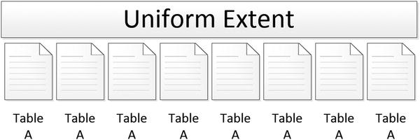
Figure 2-4. Uniform extent
Page Types
As mentioned, there are many ways in which a page can be used in the database. For each of these uses, there is a type associated with the page that defines how the page will be used. The page types available in a SQL Server database are
- File header page
- Boot page
- Page Free Space (PFS) page
- Global Allocation Map (GAM) page
- Shared Global Allocation Map (SGAM) page
- Differential Changed Map (DCM) page
- Bulk Changed Map (BCM) page
- Index Allocation Map (IAM) page
- Data page
- Index page
- Large object (Text and Image) page
The next few sections will expand on the types of pages and explain how they are used. While not every page type deals directly with indexing, all of them will be defined and explained to help provide an understanding of the total picture. With every database, there are similarities in which the pages are laid out. For instance, in the first file of every database the pages are laid out as shown in Figure 2-5. There are more page types available than the figure indicates, but as the examinations of each page type will show, only those in the first few pages are fixed. Many of the others appear in patterns that are dictated by the data in the database.

Figure 2-5. Data file pages
![]() Note Database log files don’t use the page architecture. Page structures apply only to database data files. A discussion of log file architecture is outside the scope of this book.
Note Database log files don’t use the page architecture. Page structures apply only to database data files. A discussion of log file architecture is outside the scope of this book.
File Header Page
The first page in any database data file is the file header page, shown in Figure 2-5. Since this is the first page, it is always numbered 0. The file header page contains metadata information about the database file. The information on this page includes
- File ID
- File group ID
- Current size of the file
- Max file size
- Sector size
- LSN information
There are a number of other details about the file on the file header page, but basically the information is immaterial to indexing internals.
Boot Page
The boot page is similar to the file header page in that it provides metadata information. This page, though, provides metadata information for the database itself instead of for the data file. There is one boot page per database, and it is located on page 9 in the first data file for a database (see Figure 2-5). Some of the information on the boot page includes the current version of the database, the create date and version for the database, the database name, the database ID, and the compatibility level.
One important attribute on the boot page is the attribute dbi_dbccLastKnownGood. This attribute provides the date that the last known DBCC CHECKDB completed successfully. While database maintenance isn’t within the scope of this book, regular consistency checks of a database are critical to verifying that data remains available.
Page Free Space Page
To track whether pages have space available for inserting rows, each data file contains Page Free Space (PFS) pages. These pages, which are the second page of the data file (see Figure 2-5) and located every 8,088 pages after that, track the amount of free space in the database. Each byte on the PFS page represents one subsequent page in the data file and provides some simple allocation information regarding the page; namely, it determines the approximate amount of free space on the page.
When the database engine needs to store LOB data or data for heaps, it needs to know where the next available page is and how full the currently allocated pages are. This functionality is provided by PFS pages. Within each byte are flags that identify the current amount of space that is being used. Bits 0–2 determine whether the page is in one of the following free space states:
- Page is empty
- 1 to 50 percent full
- 51 to 80 percent full
- 81 to 95 percent full
- 96 to 100 percent full
Along with free space, PFS pages also contain bits to identify a few other types of information for a page. For instance, bit 3 determines whether there are ghost records on a page. Bit 4 identifies whether the page is part of the Index Allocation Map, described later in this chapter. Bit 5 states whether the page is a mixed page. And finally, bit 6 identifies whether a page has been allocated.
Through the additional flags, or bits, SQL Server can determine what and how a page is being used from a high level. It can determine whether it is currently allocated. If not, is it available for LOB or heap data? If it is currently allocated, the PFS page then provides the first purpose described earlier in this section.
Finally, when the ghost cleanup process runs, the process doesn’t need to check every page in a database for records to clean up. Instead, the PFS page can be checked, and only those pages with ghost records need to be accessed.
![]() Note The indexes themselves handle free space and page allocation for non-LOB data and indexes. The allocation of pages for these structures is determined by the definition of the structure.
Note The indexes themselves handle free space and page allocation for non-LOB data and indexes. The allocation of pages for these structures is determined by the definition of the structure.
Global Allocation Map Page
Similar to the PFS page is the Global Allocation Map (GAM) page. This page determines whether an extent has been designated for use as a uniform extent. A secondary purpose of the GAM page is helping determine whether the extent is free and available for allocation.
Each GAM page provides a map of all subsequent extents in each GAM interval. A GAM interval consists of the 64,000 extents, or 4GB, that follow the GAM page. Each bit on the GAM page represents one extent following the GAM page. The first GAM page is located on page 2 of the database file (see Figure 2-5).
To determine whether an extent has been allocated to a uniform extent, SQL Server checks the bit in the GAM page that represents the extent. If the extent is allocated, then the bit is set to 0. When it is set to 1, the extent is free and available for other purposes.
Shared Global Allocation Map Page
Nearly identically to the GAM page is the Shared Global Allocation Map (SGAM) page. The primary difference between the pages is that the SGAM page determines whether an extent is allocated as a mixed extent. Like the GAM page, the SGAM page is also used to determine whether pages are available for allocation.
Each SGAM page provides a map of all subsequent extents in each SGAM interval. An SGAM interval consists of the 64,000 extents, or 4GB, that follow the SGAM page. Each bit on the SGAM page represents one extent following the SGAM page. The first SGAM page is located on page 3, after the GAM page of the database file (see Figure 2-5).
The SGAM pages determine when an extent has been allocated for use as a mixed extent. If the extent is allocated for this purpose and has a free page, the bit is set to 1. When it is set to 0, either the extent is not used as a mixed extent or it is a mixed extent with all pages in use.
Differential Changed Map Page
The next page to discuss is the Differential Change Map (DCM) page. This page is used to determine whether an extent in a GAM interval has changed. When an extent changes, a bit value is changed from 0 to 1. These bits are stored in a bitmap row on the DCM page with each bit representing an extent.
DCM pages are used track which extents have changed between full database backups. Whenever a full database backup occurs, all the bits on the DCM page are reset to 0. The bit then changes back to 1 when a change occurs within the associated extent.
The primary use for DCM pages is to provide a list of extents that have been modified for differential backups. Instead of checking every page or extent in the database to see whether it has changed, the DCM pages provide the list of extents to back up.
The first DCM page is located at page 6 of the data file. Subsequent DCM pages occur for each GAM interval in the data file.
Bulk Changed Map Page
After the DCM page is the Bulk Changed Map (BCM) page. The BCM page is used to indicate when an extent in a GAM interval has been modified by a minimally logged operation. Any extent that is affected by a minimally logged operation will have its bit value set to 1, and those that have not will be set to 0. The bits are stored in a bitmap row on the BCM page with each bit representing an extent in the GAM interval.
As the name implies, BCM pages are used in conjunction with the BULK_LOGGED recovery model. When the database uses this recovery model, the BCM page is used to identify extents that were modified with a minimally logged operation since the last transaction log backup. When the transaction log backup completes, the bits on the BCM page are reset to 0.
The first BCM page is located at page 7 of the data file. Subsequent BCM pages occur for each GAM interval in the data file.
Index Allocation Map Page
Most of the pages discussed so far provide information about whether there is data on the pages they cover. More important than whether a page is open and available, SQL Server needs to know whether the information on a page is associated to a specific table or index. The pages that provide this information are the Index Allocation Map (IAM) pages.
Every table or index first starts with an IAM page. This page indicates which extents within a GAM interval, discussed previously, are associated with the table or index. If a table or index crosses more than one GAM interval, there will be more than one IAM page for the table or index.
There are four types of pages that an IAM page associates with a table or index. These are data, index, large object, and small-large object pages. The IAM page accomplishes the association of the pages to the table or index through a bitmap row on the IAM page.
Besides the bitmap row, there is also an IAM header row on the IAM page. The IAM header provides the sequence number of IAM pages for a table or index. It also contains the starting page for the GAM interval that the IAM page is associated with. Finally, the row contains a single-page allocation array. This is used when less than an extent has been allocated to a table or index.
The value in understanding the IAM page is that it provides a map and root through which all the pages of a table or indexes come together. This page is used when all the extents for a table or index need to be determined.
Data Page
Data pages are likely the most prevalent type of pages in any database. Data pages are used to store the data from rows in the database’s tables. Except for a few data types, all data for a record is located on data pages. The exception to this rule is columns that store data in LOB data types. That information is stored on large object pages, discussed later in this section.
An understanding of data pages is important in relation to indexing internals. The understanding is important because data pages are the most common page that will be looked at when looking at the internals of an index. When you get to the lowest levels of the index, data pages will always be found.
Index Page
Similar to data pages are index pages. These pages provide information on the structure of indexes and where data pages are located. For clustered indexes, the index pages are used to build the hierarchy of pages that are used to navigate the clustered index. With nonclustered indexes, index pages perform the same function but are also used to store the key values that comprise the index.
As mentioned, index pages are used to build the hierarchy of pages within an index. To accomplish this, the data contained in an index page provides a mapping of key values and page addresses. The key value is the key value from the index that the first sorted row on the child table contains, and the page address identifies where to locate this.
Index pages are constructed similarly to other page types. The page has a page header that contains all the standard information, such as page type, allocation unit, partition ID, and allocation status. The row offset array contains pointers to where the index data rows are located on the page. The index data rows contain two pieces of information: the key value and a page address (these were described earlier).
Understanding index pages is important since they provide a map of how all the data pages in an index are hooked together.
Large Object Page
As previously discussed, the limit for data on a single page is 8KB. The maximum size, though, for some data types can be as high as 2GB. For these data types, another storage mechanism is required to store the data. For this there is a large object page type.
The data types that can utilize LOB pages include text, ntext, image, nvarchar(max), varchar(max), varbinary(max), and xml. When the data for one of these data types is stored on a data page, the LOB page will be used if the size of the row will exceed 8KB. In these cases, the column will contain references to the LOB pages required for the data, and it will be stored on LOB pages instead (see Figure 2-6).

Figure 2-6. Data page link to LOB page
Organizing Pages
So far you’ve looked at the low-level components that make up the internals for indexing. While these pieces are important to indexing, the structures in which these components are organized are where the value of indexing is realized. SQL Server utilizes a number of different organizational structures for storing data in the database.
The organizational structures in SQL Server 2012 are
- Heap
- B-tree
- Columnar
These structures all map to specific index types that will be discussed later in this chapter. In this section, you’ll examine each of the ways to organize pages to build that understanding.
![]() Note In the structures for organizing indexes, the levels of the index that contain index pages are considered nonleaf levels. When referencing levels that contain data pages, the levels are called leaf levels.
Note In the structures for organizing indexes, the levels of the index that contain index pages are considered nonleaf levels. When referencing levels that contain data pages, the levels are called leaf levels.
Heap Structure
The default structure for organizing pages is called a heap. Heaps occur when a B-tree structure, discussed in the next section, is not used to organize the data pages in a table. Conceptually, a heap can be envisioned to be a pile of data pages in no particular order, as shown in Figure 2-7. In the example, the only way to retrieve all of the “Madison” records is to check each page to see whether “Madison” is on the page.

Figure 2-7. Heap pile example
From an internals perspective, though, heaps are more than a pile of pages. While unsorted, heaps have a few key components that organize the pages for easy access. All heaps start with an IAM page, shown in Figure 2-8. IAM pages, as discussed, map out which extents and single-page allocations within a GAM interval are associated with an index. For a heap, the IAM page is the only mechanism for associating data pages and extents to a heap. As mentioned, the heap structure does not enforce any sort of ordering on the pages that are associated with the heap. The first page available in a heap is the first page found in the database file for the heap.

Figure 2-8. Heap structure
The IAM page lists all the data pages associated with the heap. The data pages for the heap store the rows for the table, with the use of LOB pages as needed. When the IAM page has no more pages available to allocate in the GAM interval, a new IAM page is allocated to the heap, and the next set of pages and their corresponding rows are added to the heap, as detailed in Figure 2-1. As the image shows, a heap structure is flat. From top to bottom, there is only ever one level from the IAM pages to the data pages of the structure.
While a heap provides a mechanism for organizing pages, it does not relate to an index type. A heap structure is used when a table does not have a clustered index. When a heap stores rows in a table, the rows are inserted without an enforced order. This happens because, as opposed to a clustered index, a sort order based on specific columns does not exist on a heap.
B-Tree Structure
The second available structure that can be used for indexing is the Balanced-tree, or B-tree, structure. It is the most commonly used structure for organizing indexes in SQL Server and is used by both clustered and nonclustered indexes.
In a B-tree, pages are organized in a hierarchical tree structure, as shown in Figure 2-9. Within the structure, pages are sorted to optimize searches for information within the structure. Along with the sorting, relationships between pages are maintained to allow sequential access to pages across the levels of the index.

Figure 2-9. B-tree structure
Similar to heaps, B-trees start with an IAM page that identifies where the first page of the B-tree is located within the GAM interval. The first page of the B-tree is an index page and is often referred to as the root level of the index. As an index page, the root level contains key values and page addresses for the next pages in the index. Depending on the size of the index, the next level of the index may be data pages or additional index pages.
If the number of index rows required to sort all the rows on the data pages exceeds the space available, then the root page will be followed by another level of index pages. Additional levels of index pages in a B-tree are referred to as intermediate levels. In many cases, indexes built with a B-tree structure will not require more than one or two intermediate levels. Even with a wide indexing key, millions to billions of rows can be sorted with just a few levels.
The next level of pages below the root and intermediate levels of the indexes, referred to as the nonleaf levels, is the leaf level (see Figure 2-9). The leaf level contains all the data pages for the index. The data pages are where all the key values and the nonkey values for the row are stored. Nonkey values are never stored on the index pages.
Another differentiator between heaps and B-trees is the ability within the index levels to perform sequential page reads. Pages contain previous page and next page properties in the page headers. With index and data pages, these properties are populated and can be used to traverse the B-tree to find the next requested row from the B-tree without returning to the root level of the index. To illustrate this, consider a situation where you request the rows with key values between 925 and 3,025 from the index shown in Figure 2-9. Through a B-tree, this operation can be done by traversing the B-tree down to key value 925, shown in Figure 2-10. After that, the rows through key value 3,025 can be retrieved by accessing all pages after the first page in order, finishing the operation when the last key value is encountered.

Figure 2-10. B-tree sequential read
One option available for tables and indexes is the ability to partition these structures. Partitioning changes the physical implementation of the index and how the index and data pages are organized. From the perspective of the B-tree structure, each partition in an index has its own B-tree. If a table is partitioned into three different partitions, there will then be three B-tree structures for the index.
Columnstore Structure
Columnstore, first introduced with SQL Server 2012, introduces a new organizational structure, which is based on Microsoft’s Vertipaq technology. The columnstore structure is used by the clustered and nonclustered columnstore index types. The columnstore structure makes a divergence from the traditional method of storing and indexing data from a row-wise to a column-wise format. This means that instead of storing all the values for a row with all the other values in the row, the values are stored with the values of the same column grouped together. For instance, in the example in Figure 2-11, instead of four row “groups” stored on the page, three column “groups” are stored.

Figure 2-11. Row-wise versus column-wise storage
The physical implementation of the columnstore structure does not introduce any new page types; it instead utilizes existing page types. Like other structures, a columnstore begins with an IAM page, shown in Figure 2-12. From the IAM page are LOB pages that contain the columnstore information. For each column stored in the columnstore, there are one or more segments. Segments contain up to about one million rows worth of data for the columns that they represent. An LOB page can contain one or more segments, and the segments can span multiple LOB pages.

Figure 2-12. Columnstore structure
Within each segment is a hash dictionary that is used to map the data that comprises the segment of the columnstore. The hash dictionary also contains the minimum and maximum values for the data in the segment. This information is used by SQL Server during query execution to eliminate segments during query execution.
One of the advantages of the columnstore structure is its ability to leverage compression. Since each segment of the columnstore structure contains the same type of data, both from a data type and from a contents perspective, SQL Server has a greater likelihood of being able to utilize compression on the data. The compression used by the columnstore is similar to page-level compression. It utilizes dictionary compression to remove similar values throughout the segment. There are two main differences between page and columnstore compression. First, while page compression is optional, columnstore compression is mandatory and cannot be disabled. Second, page compression is limited to compressing the values on a single page. Alternately, columnstore compression is for the entire segment, which may span multiple pages or could have multiple segments on the same page. Regardless of the number of pages or segments on a page, columnstore compression is contained to the segment.
Another advantage to the columnstore is that only the columns requested from the columnstore are returned. I often remind developers not to use SELECT * when querying databases; instead, they are asked to request only the columns that are required. Unfortunately, even when this practice is followed, all the columns for the row are still read from disk into memory. The practice reduces some network traffic and streamlines execution, but it doesn’t assist with the bottleneck of reading data from disk. Columnstore addresses this issue by reading only from the columns that are requested and moving that data into memory. Along these same lines, according to Microsoft, queries often access only 10 to 15 percent of the available columns in a table.1 The reduction in the columns retrieved from a columnstore structure will have a significant impact on performance and I/O.
While the columnar structure is unchanged between clustered and nonclustered columnstore indexes, there are a few points of distinction between the two that are important to be aware of. A clustered columnstore index has an additional structure, called the deltastore, which allows write operations on the index. While segments of both types of columnstore are read-only, the deltastore allows insert, update, and delete actions against the index. Also, a clustered columnstore is the base copy of the data; it doesn’t have a clustered index or heap that it relies on for a full copy of the data. All data is stored in a clustered columnstore index. Alternatively, the nonclustered columnstore index requires a traditional clustered index on the data it is using and generally represents a duplication of the data in the database.
![]() Note The columnstore structure and related columnstore index are available only in SQL Server Enterprise, Evaluation, and Developer editions, and only in 2014 and later releases.
Note The columnstore structure and related columnstore index are available only in SQL Server Enterprise, Evaluation, and Developer editions, and only in 2014 and later releases.
Examining Pages
The first part of this chapter outlined the types of pages found in SQL Server databases. On top of that, you’ve looked at the structures available for organizing and managing the relationship between pages within your databases. In this next section, you will look at the tools available for examining pages in your database. The purpose of using these tools is to provide a foundation from which you’ll be able to look at the behaviors of indexes in this chapter and throughout the rest of the book. Also, this will provide you with the knowledge to do your own exploration of indexes in your environment.
![]() Warning The tools used in this section are undocumented and unsupported. They do not appear in Books Online, and their functionality can change without notice. That being said, these tools have been around for quite some time, and there are many blog posts that describe their behavior. You can find additional resources for using these tools at www.sqlskills.com.
Warning The tools used in this section are undocumented and unsupported. They do not appear in Books Online, and their functionality can change without notice. That being said, these tools have been around for quite some time, and there are many blog posts that describe their behavior. You can find additional resources for using these tools at www.sqlskills.com.
DBCC EXTENTINFO
The DBCC command DBCC EXTENTINFO provides information about extents allocations that occur within a database. The command can be used to identify how extents have been allocated and whether the extents being used are mixed or uniform. Listing 2-1 shows the syntax for using DBCC EXTENTINFO. When using the command, there are four parameters that can be populated; these are defined in Table 2-1.
Table 2-1. DBCC EXTENTINFO Parameters
|
Parameter |
Description |
|---|---|
|
database_name | database_id |
Specifies either the database name or the database ID where the page will be retrieved. If the value 0 is provided for this parameter or the parameter is not set, then the current database will be used. |
|
table_name | table_object_id |
Specifies which table to return in the output by providing either the table name or the object_ID for the table. If no value is provided, the output will include results for all tables. |
|
index_name | index_id |
Specifies which index to return in the output by providing either the index name or the index_ID. If -1 or no value is provided, then the output will include results for all indexes on the table. |
|
partition_id |
Specifies which partition of the index to return in the output by providing the partition number. If 0 or no value is provided, then the output will include results for all partitions on the index. |
When executing DBCC EXTENTINFO, a dataset is returned. The results include the columns defined in Table 2-2. For every extent allocation, there will be one row in the results. Since extents are comprised of eight pages, there can be as many as eight allocations for an extent when there are single-page allocations, such as when mixed extents are used. When uniform extents are used, there will be only one extent allocation and one row returned for the extent.
Table 2-2. DBCC EXTENTINFO Output Columns
|
Parameter |
Description |
|---|---|
|
file_id |
File number where the page is located. |
|
page_id |
Page number for the page. |
|
pg_alloc |
Number of pages allocated from the extent to the object. |
|
ext_size |
Size of the extent. |
|
object_id |
Object ID for the table. |
|
index_id |
Index ID associated with the heap or index. |
|
partition_number |
Partition number for the heap or index. |
|
partition_id |
Partition ID for the heap or index. |
|
iam_chain_type |
The type of IAM chain the extent is used for. Values can be in-row data, LOB data, and overflow data. |
|
pfs_bytes |
Bytes array that identifies the amount of free space, whether there are ghost records, whether the page is an IAM page, whether it is allocated, and whether it is part of a mixed extent. |
To demonstrate how the command works, let’s walk through a couple examples to observe how extents are allocated. In the first example, shown in Listing 2-2, you will create a database named Chapter2Internals. In the database, you will create a table named dbo.IndexInternalsOne with a table definition that inserts one row per data page. Into the table you will first insert four records. The last statement in Listing 2-2 is the DBCC EXTENTINFO command against dbo.IndexInternalsOne.
In the results from the DBCC command, shown in Figure 2-13, you can see that there were four pages allocated to the table. The items of interest in these results are the pg_alloc and ext_size columns. Both of these columns should have the number 1 in your results. This means that one page of the extent was allocated and used by the table. Even though pages 280, 281, and 282 are on the same extent, the pages are allocated separately because each insert was in a separate transaction. You can determine that the pages are on the same extent by dividing the page number by 8. In this case, pages 280, 281, and 282 are on the 35th extent in the database. The fourth page allocated to the table shows another interesting aspect of single-page allocations. The page allocated is in the 30th extent. This demonstrates that single-page allocations to a table with less than eight pages may not be in the same extent in the database and may not even be on neighboring extents.

Figure 2-13. DBCC EXTENTINFO for eight pages in dbo.IndexInternalsOne
Now you’ll expand the example a bit further. For the second example, you’ll perform two more sets of inserts into the table dbo.IndexInternalsOne, shown in Listing 2-3. In the first insert, you’ll insert two records, which will require two pages. The second insert will insert another four rows, which will result in four additional pages. The final count pages for the table will be ten, which should change SQL Server from allocating pages via mixed extents to uniform extents.
The results from the second example, shown in Figure 2-14, show a couple of interesting pieces of information on how mixed and uniform extents are allocated. First, even though the first insert added two rows resulting in two new pages, numbered 285 and 286, these pages were still allocated one at a time, which is why it’s called single-page allocation. Next is the insert that increased the size of the table by another four pages. Looking at the results, the four pages added were not allocated identically. The first two pages, numbered 285 and 286, were added as single-page allocations. The other two pages, starting with page number 304, were added in an extent allocation that contained eight pages with two pages currently allocated, shown in columns ext_size and pg_alloc, respectively. One of the key takeaways in this example is that when the number of pages exceeds eight for a table or index, allocations change from mixed to uniform and previous allocations are not re-allocated.

Figure 2-14. DBCC EXTENTINFO for ten pages in dbo.IndexInternalsTwo
Now let’s look at how to remove the initial single-page allocations in the mixed extent from the table or index. Accomplishing this change is relatively simple: the table or index just needs to be rebuilt. The code in Listing 2-4 will rebuild the table dbo.IndexInternalsOne and then execute DBCC EXTENTINFO.
In this third example, the rebuild of the table removed all the single-page allocations. Now instead of nine extent allocations, there are only two allocations (see Figure 2-15). Both allocations are for extents that contain eight pages. The one peculiar item in the results is the first allocation that has nine of eight pages allocated. The extra page allocated is the IAM page associated with the table or index. When a table or index begins with uniform extents, the IAM page is included in the count with the first extent. The reason that uniform extents are used is that SQL Server was able to determine during the insert that the number of pages allocated would exceed a single extent and skipped mixed extent allocations.

Figure 2-15. DBCC EXTENTINFO for dbo.IndexInternalsOne after REBUILD
In the last three examples, you worked with an example that started with inserts that inserted one page per transaction. In the next example, you’ll use DBCC EXTENTINFO to observe the behavior when more than eight pages are inserted into a table in the first transaction. Using the code in Listing 2-5, you’ll build a new table named dbo.IndexInternalsTwo. Into this table, you’ll insert nine rows, which will require nine pages to be allocated. Then you’ll execute the DBCC command to see the results.
As you can see in the results, shown in Figure 2-16, it doesn’t matter how large the initial insert into a table is because the first pages allocated to the table or index will use single-page allocation from mixed extents. Not until the ninth page is needed does the table make the switch from mixed to uniform extents, shown by the extent size of eight on the last row. Regardless of the size of the insert, extents are initially allocated one at a time.

Figure 2-16. DBCC EXTENTINFO for dbo.IndexInternalsTwo
As these examples have shown, DBCC EXTENTINFO can be extremely useful for investigating how pages are allocated to tables and indexes. Through the examples, you were able to verify the page and extent allocation information that was discussed earlier in this chapter. Using the DBCC command can be extremely useful when trying to investigate issues related to fragmentation and how pages have been allocated. In Chapter 6, you’ll look at how to use this command to identify potential excessive use of extents.
DBCC IND
The next command that can be used to investigate indexes and their associated pages is DBCC IND. This command returns a list of all the pages associated with the requested object, which can be scoped to the database, table, or index level. Listing 2-6 shows the syntax for using DBCC IND. When using the command, there are three parameters that can be populated; these are defined in Table 2-3.
Table 2-3. DBCC IND Parameters
|
Parameter |
Description |
|---|---|
|
database_name | database_id |
Specifies either the database name or the database ID where the page list will be retrieved. If the value 0 is provided for this parameter or the parameter is not set, then the current database will be used. |
|
table_name | table_object_id |
Specifies which table to return in the output by providing either the table name or the object_ID for the table. If no value is provided, the output will include results for all tables. |
|
index_name | index_id |
Specifies which index to return in the output by providing either the index name or the index_ID. If -1 or no value is provided, the output will include results for all indexes on the table. |
DBCC IND returns a dataset when executed. For every page that is allocated to the requested objects, one row is returned in the dataset; the columns are defined in Table 2-4. Unlike the previous DBCC EXTENTINFO, DBCC IND does explicitly return the IAM page in the results.
Table 2-4. DBCC IND Output Columns
|
Column |
Description |
|---|---|
|
PageFID |
File number where the page is located. |
|
PagePID |
Page number for the page. |
|
IAMFID |
File ID where the IAM page is located. |
|
IAMPID |
Page ID for the page in the data file. |
|
ObjectID |
Object ID for the associated table. |
|
IndexID |
Index ID associated with the heap or index. |
|
PartitionNumber |
Partition number for the heap or index. |
|
PartitionID |
Partition ID for the heap or index. |
|
iam_chain_type |
The type of IAM chain the extent is used for. Values can be in-row data, LOB data, and overflow data. |
|
PageType |
Number identifying the page type. These are listed in Table 2-5. |
|
IndexLevel |
Level at which the page exists in the page organizational structure. The levels are organized from 0 to N, where 0 is the lowest level of the index and N is the index root. |
|
NextPageFID |
File number where the next page at the index level is located. |
|
NextPagePID |
Page number for the next page at the index level. |
|
PrevPageFID |
File number where the previous page at the index level is located. |
|
PrevPagePID |
Page number for the previous page at the index level. |
Within the results from DBCC EXTENTINFO is a PageType column. This column identifies what type of page is returned through the DBCC command. The page types can include data, index, GAM, or any other of the page types discussed earlier in the chapter. Table 2-5 shows a full list of the page types and the value identifying the page type.
Table 2-5. Page Type Mappings
|
Page Type |
Description |
|---|---|
|
1 |
Data page |
|
2 |
Index page |
|
3 |
Large object page |
|
4 |
Large object page |
|
8 |
Global Allocation Map page |
|
9 |
Share Global Allocation Map page |
|
10 |
Index Allocation Map page |
|
11 |
Page Free Space page |
|
13 |
Boot page |
|
15 |
File header page |
|
16 |
Differential Changed Map page |
|
17 |
Bulk Changed Map page |
The primary benefit of using DBCC IND is that it provides a list of all pages for a table or index with their locations in the database. You can use this to help investigate how indexes are behaving and where pages are ending up. To put this information into action, here are a couple demos.
For the first example, you’ll revisit the tables created in the previous section and examine the output for each of these in comparison to the DBCC EXTENTINFO output. The code example includes DBCC IND commands for IndexInternalsOne and IndexInternalsTwo, shown in Listing 2-7. The database ID passed in is 0 for the current database, and the index ID is set to -1 to return pages for all indexes.
In the DBCC EXTENTINFO examples, there were two extent allocations for the table IndexInternalsOne, shown in Figure 2-15. These results show that there were 11 pages allocated to the table. The DBCC IND results, shown in Figure 2-17, detail all the pages that were part of the previous two extent allocations.

Figure 2-17. DBCC IND for dbo.IndexInternalsOne
In these results, there was a single IAM page and ten data pages allocated to the table. Where DBCC EXTENTINFO provided page 280 as the start of the extent allocations, containing nine pages, it was not possible to identify where the IAM page was based on that. It was instead in another extent that the results did not list, and the results for DBCC IND identify it as being on page 270.
The next set of results from the example shows the output for DBCC IND against dbo.IndexInternalsTwo. These results, shown in Figure 2-18, are quite similar with the exception of the IAM page. Reviewing the results for DBCC EXTENTINFO, in Figure 2-14, the extent allocations account for only nine pages being allocated to the table. In the results for dbo.IndexInternalsTwo, there are ten pages allocated, with one of them being the IAM page. The benefit of using DBCC IND for listing the page for an index is that you get the exact page numbers without having to make any guesses. Also, note that the index level in the results returns as level 0 with no intermediate levels. As stated earlier, heap structures are flat, and the pages are in no particular order.

Figure 2-18. DBCC IND for dbo.IndexInternalsTwo
As mentioned, the tables in the previous example were organized in a heap structure. For the next example, you’ll observe what the output from DBCC IND is when examining a table with a clustered index. In Listing 2-8, first the table dbo.IndexInternalsThree is created with a clustered index on the RowID column. Then, you’ll insert four rows. Finally, the example executes DBCC IND on the table.
Figure 2-19 shows the results from this example involving dbo.IndexInternalsThree. Notice the change in how IndexLevel is being returned as compared to the previous example (Figure 2-18).

Figure 2-19. DBCC IND for dbo.IndexInternalsThree
In this example, the index level for the third row in the results has an IndexLevel of 1 and also a PageType of 2, which is an index page. With these results, there is enough information to rebuild the B-tree structure for the index, as shown in Figure 2-20. The B-tree starts with the IAM page, which is page number 1:281. This page is linked to page 1:282, which is an index page at index level 1. Following that, pages 1:280, 1:285, 1:286, and 1:287 are at index level 0 and doubly linked to each other.

Figure 2-20. DBCC IND for dbo.IndexInternalsThree
Through both of these examples, you examined how to use DBCC IND to investigate the pages associated with a table or an index. As the examples showed, the command provides the information on all the pages of the table or index, including the IAM page. These pages include the page numbers to identify where they are in the database. The relationships between the pages are also included, even the next and previous page numbers that are used to navigate the index for B-tree indexes.
sys.dm_db_database_page_allocations
An alternative to using DBCC IND is sys.dm_db_database_page_allocations. This dynamic management function (DMF) provides replacement functionality to DBCC IND with additional capabilities that the DBCC command does not provide. For instance, since the source of the results is output from a query, the results can be filtered, formatted, and joined to other metadata in the database and server.
The DMF also provides more data than DBCC IND. While DBCC IND provides only page allocations for the object, it actually provides only page allocations that have data on them. There can be pages allocated to an index without data on them, which sys.dm_db_database_page_allocations will return.
Listing 2-9 shows the syntax for using sys.dm_db_database_page_allocations. The execution required five parameters, which are defined in Table 2-6.
Table 2-6. Parameters for sys.dm_db_database_page_allocations
|
DMF Column |
Description |
|---|---|
|
@DatabaseId |
Database from which to return the page listing for tables and indexes. The parameter is required and accepts the use of the DB_ID() function. |
|
@TableId |
Object_id for the table from which to return the page listing. The parameter is required and accepts the use of the OBJECT_ID() function. NULL can also be used to return all tables. |
|
@IndexId |
Index_id from the table that the page list is from. The parameter is required and accepts the use of NULL to return information for all indexes. |
|
@PartionId |
ID of the partition that the page list is returning. The parameter is required and accepts the use of NULL to return information for all indexes. |
|
@Mode |
Defines the mode for returning data; the options are DETAILED and LIMITED. With LIMITED, the information is limited to page metadata, such as page allocation and relationships information. Under the DETAILED mode, additional information is provided, such as page type and interpage relationship chains. |
There are many similarities and differences between using the DMF and DBCC IND. For starters, the columns between the two overlap in a number of places (though the names of columns do differ), as shown in Table 2-7. Every column is covered in sys.dm_db_database_page_allocations for those returned by DBCC IND. To demonstrate the similarities, use the code provided in Listing 2-10. If you compare the outputs, you’ll note that they are nearly identical; there are a few instances where NULL and 0 are returned differently.
Table 2-7. Columns for sys.dm_db_database_page_allocations with DBCC Mappings
|
DMF Column |
DBCC Column |
Description |
|---|---|---|
|
object_id |
ObjectID |
Object ID for the table or view |
|
index_id |
IndexID |
ID for the index |
|
partition_id |
PartitionNumber |
Partition number for the index |
|
rowset_id |
PartitionID |
Partition ID for the index |
|
allocation_unit_type_desc |
iam_chain_type |
Description of the allocation unit |
|
allocated_page_iam_file_id |
IAMFID |
File ID for the index allocation map page associated to the page |
|
allocated_page_iam_page_id |
IAMPID |
Page ID for the index allocation map page associated to the page |
|
allocated_page_file_id |
PageFID |
File ID of the allocated page |
|
allocated_page_page_id |
PagePID |
Page ID for the allocated page |
|
page_type |
PageType |
Page type ID for the allocated page |
|
page_level |
IndexLevel |
Level of the page in B-tree index |
|
next_page_file_id |
NextPageFID |
File ID for the next page |
|
next_page_page_id |
NextPagePID |
Page ID for the next page |
|
previous_page_file_id |
PrevPageFID |
File ID for the previous page |
|
previous_page_page_id |
PrevPagePID |
Page ID for the previous page |
Besides the columns that match, there are a number of additional columns in the DMF. These columns, defined in Table 2-8, provide metadata on pages and information on the extents they tie into. Overall, this provides the ability to see and understand how and what pages have been assigned and allocated to a table.
Table 2-8. Additional Columns for sys.dm_db_database_page_allocations
|
DMF Column |
Description |
|---|---|
|
database_id |
ID of the database |
|
allocation_unit_id |
ID of the allocation unit |
|
allocation_unit_type |
Type of allocation unit |
|
data_clone_id |
Unknown |
|
clone_state |
Unknown |
|
clone_state_desc |
Unknown |
|
extent_file_id |
File ID of the extent |
|
extent_page_id |
Page ID for the extent |
|
is_allocated |
Indicates whether a page is allocated |
|
is_iam_page |
Indicates whether a page is the index allocation page |
|
is_mixed_page_allocation |
Indicates whether a page is allocated |
|
page_free_space_percent |
Percentage of space free on the page |
|
page_type_desc |
Description of the page type |
|
is_page_compressed |
Indicates whether the page is compressed |
|
has_ghost_records |
Indicates whether the page has ghost records |
DBCC PAGE
The last command available for examining pages is DBCC PAGE. While the other two commands provide information on the pages associated with tables and indexes, the output from DBCC PAGE provides a look at the contents of a page. Listing 2-11 shows the syntax for using DBCC PAGE.
The DBCC PAGE command accepts a number of parameters. Through the parameters, the command is able to determine the database and specific page requested, which is then returned in the requested format. Table 2-9 details the parameters for DBCC PAGE.
Table 2-9. DBCC PAGE Parameters
![]() Note By default, the DBCC PAGE command outputs its messages to the SQL Server event log. In most situations, this is not the ideal output mechanism. Trace flag 3604 allows you to modify this behavior. By utilizing this trace flag, the output from the DBCC statements returns to the Messages tab in SQL Server Management Studio.
Note By default, the DBCC PAGE command outputs its messages to the SQL Server event log. In most situations, this is not the ideal output mechanism. Trace flag 3604 allows you to modify this behavior. By utilizing this trace flag, the output from the DBCC statements returns to the Messages tab in SQL Server Management Studio.
Through DBCC PAGE and its print options, everything that is on a page can be retrieved. There are a few reasons why you might want to look at the contents of a page. To start with, looking at an index or data page can help you understand why an index is behaving in one manner or another. You gain insight into how the data within the row is structured, which may cause rows to be larger than expected. The sizes of rows do have an important impact on how indexes behave since as a row gets larger, the number of pages required to store the indexes increase. An increase in the number of pages for an index increases the resources required to use the index, which results in longer query times and, in some cases, a change in how or which indexes will be utilized. Another reason to use DBCC PAGE is to observe what happens to a data page when certain operations occur. As the examples later in this chapter will illustrate, DBCC PAGE can be used to uncover what happens during page splits and forwarded record operations.
To help demonstrate how to use DBCC PAGE, you’ll run through a few demonstrations with each of the print options. These demos will be based on the code in Listing 2-12, which uses sys.dm_db_database_page_allocations to identify page numbers for the examples. For each example, you’ll look at some of the ways the results can differ between page types. While the page numbers in your database may differ slightly, the demos are based on an IAM page of 309, index page of 310, and data pages of 308 and 311, as shown in Figure 2-21.

Figure 2-21. Page allocations for dbo.IndexInternalsFour
Page Header Only Print Option
The first print option available for DBCC PAGE is the page header only where print_option equals 0. With this option, only the page header is returned in the output from the DBCC command. The page header is returned with all DBCC PAGE requests; using this option just limits the results to only the page header. Two sections are returned as part of the page header.
The first section returned is the buffer information. The buffer provides information on where the page is currently located in memory in SQL Server. To read a page, the page must first be retrieved from disk and placed in memory. This section provides the address that could be used to find the memory location of the page.
The second section is the actual page header. The page header contains a number of attributes that describe the page and the contents of the page. Not all the attributes are currently in use by SQL Server, but there are a number of attributes that are worth understanding. These key attributes are listed and defined in Table 2-10.
Table 2-10. Page Header Key Attribute Definitions
|
Attribute |
Definition |
|---|---|
|
m_pageId |
File ID and page number for the page. |
|
m_type |
The type of page returned; see the page type list in Table 2-5. |
|
Metadata: AllocUnitId |
Allocation unit ID from that maps the catalog view sys.allocation_units. |
|
Metadata: PartitionId |
Partition ID for the table or index. This maps to partition_ID in the catalog view sys.partitions. |
|
Metadata: ObjectId |
Object ID for the table. This maps to the object_ID in the catalog view sys.tables. |
|
Metadata: IndexId |
Index ID for the table or index. This maps to the index_ID in the catalog view sys.indexes. |
|
m_prevPage |
Previous page in the index structure. This is used in B-tree indexes to allow reading sequential pages along index levels. |
|
m_nextPage |
Next page in the index structure. This is used in B-tree indexes to allow reading sequential pages along index levels. |
|
m_slotCnt |
Number of slots, or rows, on the page. |
|
Allocation Status |
Lists the locations of the GAM, SGAM, PFS, DIFF (or DCM), and ML (or BCM) pages for the page requested. It also includes the status for each from those metadata pages. |
To demonstrate the use of DBCC PAGE for the page header–only option, the code in Listing 2-13 can be used. Your results should be similar to those in Figure 2-22. In these results, you can see the page number at the top of the page indicating that it is page 1:310. The m_type is 2, which translates to being an index page. The m_slotCnt shows that there are two rows on the page. Referring to Figure 2-21, the row count would correlate to the two index records needed to map data pages 1:308 and 1:311 to the index. Finally, the allocations statuses show that the page is allocated on the GAM page, it is part of mixed extent (per PFS page), and the page has been changed since the last full backup (per the DCM page).

Figure 2-22. DBCC PAGE output for page header–only print option
As the page header–only option shows, there is a lot of useful information in the page header. In fact, you are provided with enough information to envision how this page relates to the other pages in the index and the extent it occupies.
The next print option available for DBCC PAGE is the hex rows print option, where print_option equals 1. This print option expands on the previous option adding into the output an entry for every slot on the page and the offset array that describes the location of each slot on the page.
The data section of the page repeats for every row that is on the page and contains all the metadata and the data associated with that row. For the metadata, the row includes the slot number, page offset, record type, and record attributes. This information helps define the row and what contributes besides the size of the data to the row size. At the end of the slot is a memory dump of the row. The memory dump displays the row in a hex format that, while not easily read by humans, contains all the data for the row. For more on the attributes and their definitions, see Table 2-11.
Table 2-11. Hex Rows Key Attribute Definitions
|
Attribute |
Definition |
|---|---|
|
Slot |
The position of the row on the page. The count is 0 based and starts immediately after the page header. |
|
Offset |
Physical byte location of the row on the page. |
|
Length |
The length of the row on the page. |
|
Record Type |
The type of row. Some possible values are INDEX_RECORD and PRIMARY_RECORD. |
|
Record Attributes |
List of attributes on the row that contribute to the size of the row. These can include the NULL_BITMAP and VARIABLE_COLUMNS array. |
|
Record Size |
The length of the row on the page. |
|
Memory Dump |
The memory location for the data on the page. For the hex rows option, it is limited to the information in that slot. The memory address is provided, and afterward a hex dump of the data is stored in the slot. |
The offset array is the last section of information included in the hex row option results. The offset array contains two pieces of information for each row on the table. The first piece of information is the slot number with its hex representation. The second piece is the byte location for the slot on the page. With these two pieces of information, any row on the page can be located and returned.
For the hex rows example, you’ll continue to investigate the index page (1:279) that you looked at in the previous section. This time, you’ll use the hex rows print option, which is when a print_option of 1 is used in DBCC PAGE, as shown in Listing 2-14.
The results for the DBCC PAGE command will be longer than the previous execution since this time it includes the row data with the page header. To focus on the new information, the buffer and page header results have been excluded in the sample output in Figure 2-23. In the data section, there are two slots shown, slot 0 and slot 1. These slots map to the two index rows on the page, which can be verified through the record type of INDEX_RECORD for each of the rows. The hex data for the rows contains the page and range information for the index record, but that isn’t translated with this print option. The last section has the offset table containing the slot information for both of the rows on the table. Note that the offset ends with 0 and counts up from the bottom. This matches to how the offset array was described earlier in the chapter. The rows start after the header incrementing up, while the offset array starts at the end of the page incrementing backward. In this manner, new rows can be added to the table without reorganizing the page.

Figure 2-23. DBCC PAGE output for hex rows print option
The hex row print option is a bit more useful than the first print option. It includes the page header information but expands on it to provide insight into the actual rows on the page. This information can prove valuable when you want to look at a row to determine its size on the page and why it may be larger than expected.
Hex Data Print Option
The third print option available for DBCC PAGE is the hex data print option, where print_option equals 2. This print option, like the previous option, starts with the output from the page header–only print option and adds to it. The information added through this option includes the hex output of the data section of the page and the offset array. With the data section, the page is output complete and unformatted as it appears on the actual page. The output in this format can be useful when you want to see the page in its raw form.
To demonstrate the hex data print option, you’ll use the script in Listing 2-15. In it the DBCC PAGE command is used to retrieve the page from dbo.IndexInternalsFour that contains the last row. This row contains 25 fives in the FillerData column.
In the results, shown in Figure 2-24, the output contains a large block of characters in the data section. The block contains three components. On the far left is page address information, such as 000000002F00A000. The page address identifies where on the page the information is located. The middle section contains the hex data that is contained in that section of the page. The right side of the character block contains the character representation of the hex data. For the most part, this data is not legible, except when it comes to character data being stored from character data types, such as char and nchar. The sixth row of the character data shows the start of the 25 fives with the value wrapping to the next line.

Figure 2-24. DBCC PAGE output for hex data print option
Initially, the hex data print option may seem less useful than the other print options. In many situations, this will be the case. The true value in this print option is that DBCC PAGE doesn’t try to interpret the page for you. It displays the page as is. With the other print options, the output will sometimes be reordered to conform to expect slot orders; an example of this is demonstrated in Chapter 8.
Row Data Print Option
The last print option available for DBCC PAGE is the row data print option, where print_option equals 3. The output from this print option can change depending on the type of page that is being requested. The basic information returned for most pages is identical to that returned from the hex rows print option: the data split per row in the hex format. The output varies, though, when it comes to data pages and index pages. For these page types, this print option provides some extremely useful information about the page.
![]() Note You can use the WITH TABLERESULTS option with DBCC PAGE to output the results from the command to a resultset instead of messages. This option is useful when you want to insert the results returned from the DBCC command into a table.
Note You can use the WITH TABLERESULTS option with DBCC PAGE to output the results from the command to a resultset instead of messages. This option is useful when you want to insert the results returned from the DBCC command into a table.
To show the differences between the data and index page outputs, let’s walk through another example. This example will use the table dbo.IndexInternalsFour that was created in Listing 2-10. In the demo for this print option, shown in Listing 2-16, you’ll execute DBCC PAGE against one of the data pages and the index page for the table.
Comparing the results from the data page, shown in Figure 2-25, to the output from the hex data print option, shown in Figure 2-24, there is one major difference. Underneath the hex memory dump for the slot, all the column details from the row are decoded and presented in a legible format. It starts with Slot 0 Column 1, which contains the RowID column, which it shows to have a value of 5. The next column, Column 2, is the FillerData column, which contains 25 fives. For each of these columns, the physical length is noted along with the offset of the value within the row. The last value provided on the data section of the page is the KeyHashValue. This value isn’t actually stored on the page. Instead, it is a hash value that was created when the page was placed in memory based on the keys on the page. This value is shown in tools that are used by SQL Server to report information about pages back to the end user; you may have seen this value before while investigating deadlocks.

Figure 2-25. DBCC PAGE output for row data print option for data page
With the index page, there isn’t a change in the message output from other page types. Instead, the difference with this page is the resultset. Instead of just a message output, a table is also returned. The table returns one row for every index row on the page. Reviewing the output for the index page, shown in Figure 2-26, there are two rows returned. The first row indicates that page 1:308 is the child page to the index page. It also shows that the key value for the index is RowID, which is NULL for the first index row. This means that this is the start of the index and no values are limiting the first values on the child page. The second row maps to page 1:311 with a key value of 5. In this case, the key value indicates that the first row on the child page has a RowID of 5. Since the key value can change from index to index, the results from the DBCC PAGE command with these options will change as well. For every index variation, the output will return the relevant values for the index.

Figure 2-26. DBCC PAGE output for row data print option for index page
The row data print option is one of the most useful options for the DBCC PAGE command. For data pages, it provides total insight into the data stored on the page, how much space it takes up, and its position. This allows you a direct line into understanding why only certain rows may be fitting on the page and why, for instance, a page split may have occurred. The resultset from the index page output is equally as useful. The ability to map the index rows to pages and return the key values can provide much insight into how the index is organized and how the pages are laid out.
Page Fragmentation
As discussed throughout this chapter, SQL Server stores information in the database on 8KB pages. In general, records in tables are limited to that size; if they are smaller than 8KB, SQL Server stores more than one record per page. One of the problems with storing more than a single record per page is handling situations where the total size of all the records on a page exceeds 8KB of space. In these situations, SQL Server must change how the records on a page are stored. Depending on how the pages are organized, there are two ways in which SQL Server will handle the situations: forwarded records and page splits.
![]() Note This discussion does not consider two situations where single records can be larger than a page. These other situations are row overflow and large objects. With row overflow, SQL Server will allow a single record on a page to exceed the 8KB in certain situations. Also, when large object values exceed the 8KB size, they utilize LOB pages instead of data pages. These do not have a direct impact on the page fragmentation discussed in this section.
Note This discussion does not consider two situations where single records can be larger than a page. These other situations are row overflow and large objects. With row overflow, SQL Server will allow a single record on a page to exceed the 8KB in certain situations. Also, when large object values exceed the 8KB size, they utilize LOB pages instead of data pages. These do not have a direct impact on the page fragmentation discussed in this section.
Forwarded Records
The first method for managing records when they exceed the size of a data page is through forwarded records. This method applies only when the heap structure is used. With forwarded records, when a row is updated and no longer fits on the data page, SQL Server will move that record to a new data page in the heap and add pointers between the two locations. The first pointer identifies the page on which the record now exists, often called the forwarded record pointer. The second is on the new page, pointing back to the original page on which the forwarded record existed; it’s called the back pointer.
As an example of how this works, let’s walk through a logical example of how forwarding operates. Consider a page, numbered 100, that exists on a table using a heap (see Figure 2-27). This page has four rows on it, and each row is approximately 2KB in size, totaling 8KB in space used. If the second row is updated to 2.5KB in size, it will no longer be able to fit on the page. SQL Server selects another page in the heap or allocates a new page to the heap, the page numbered 101 in this case. The second row is then written to that page, and the pointer to the new page replaces the row on page 100.

Figure 2-27. Forward record process diagram
Taking this logical example further, the next thing to do is examine how records are forwarded on a table. For the example, create a table named dbo.HeapForwardedRecords, shown in Listing 2-17. To represent the rows from the logical example, you’ll use the sys.objects table to add 24 rows to dbo.HeapForwardedRecords. Each of these rows has a RowID to identify the row and 2,000 characters, resulting in four rows per page in the table. Using sys.dm_db_index_physical_stats, you can verify (see Figure 2-28) that there are six pages in the table with a total of 24 records.

Figure 2-28. Physical state of dbo.HeapForwardedRecords before forwarding records
The next step in the demonstration is to cause forward records in the table. To do this, you’ll update every other row in the table to expand the values of FillerData from 2,000 to 2,500 characters, shown in Listing 2-18. As a result, two of the rows will be too large to fit in the space remaining on the pages where these rows are located. Instead of 8KB of data, there will be about 9KB being written to the 8KB page.
As a result, SQL Server will need to move records off the page to complete the updates. Since moving one of the records off the page will leave enough room on the page for the second row, only one record will be forwarded. The output from sys.dm_db_index_physical_stats (see Figure 2-29) verifies that this is the case. The page count increases to nine, and six records are logged as being forwarded. One item of particular interest is the record count. While the number of rows in the table did not increase, there are now six additional records in the table. This is because the original record for the row is still in the original position with a pointer to another record elsewhere that contains the data for the row.

Figure 2-29. Physical state of dbo.HeapForwardedRecords after forwarding records
The problem with forwarded records is that it causes rows in the table to have records in two locations, resulting in an increase in the amount of I/O activity required when retrieving data from and writing data to the table. The larger the table and the higher the number of forwarded records, the more likely that forwarded records can have a negative impact on performance.
Page Splits
The second approach for handling pages where the size of the rows on the page exceeds the size of the page is the performing the page split. A page split is used on any index that is implemented under the B-tree index structure, which includes clustered and nonclustered indexes. With page splits, if a row is updated to a size that will no longer fit on the data page on which it currently exists, SQL Server will take half the records on the page and place them on a new page. Then SQL Server will attempt to write the data for the row to the page again. If the data will then fit on the page, the page will be written. If not, then the process will be repeated until it fits on the page.
To explain how page splits operate, let’s walk through an update that results in a page split. Similar to the previous section, consider a table with a page numbered 100 (see Figure 2-30). There are four rows stored on page 100, and each is approximately 2KB in size. Suppose that one of the rows, such as the second row, is updated to 2.5KB in size. The data for the page will be 8.5KB, which exceeds the available space, which causes a page split to occur. To split the page, a new page is allocated, numbered 101, and half the rows on the page (the third and fourth row) are written to the new page. At this point, the second row can be written to the page since there is now 4KB of open space on the page.

Figure 2-30. Page split process diagram
To demonstrate how page splits occur on a table, let’s walk through an example similar to the one already described, which causes page splits to occur on the table. To start the example, create the table dbo.ClusteredPageSplits, provided in Listing 2-19. Into this table you’ll insert 24 records that are about 2KB in length. This should result in four rows per page and six data pages allocated to the table. Look at the information on index level 0, which is the leaf level. Since the table is using a B-tree, through the clustered index there will be an additional page that is used for the index tree structure. On index level 1, there are six records, which reference the six pages in the index. You can confirm this information with Figure 2-31.

Figure 2-31. Physical state of dbo.ClusteredPageSplits before page splits
Causing the page splits on the table can be done by updating some of the records to exceed the size of the page. You’ll do this by issuing an UPDATE statements that increases the FillerData column in every other row from 2,000 to 2,500 characters in length, using the script in Listing 2-20. The resulting rows on each page will be 9KB in size, which, like the previous example, exceeds the available page size, thus causing SQL Server to use page spits to free up space on the page.
Investigating the results (Figure 2-32) after the page splits have occurred shows the effect of the page splits on the table. For starters, instead of 6 pages at the leaf level of the index, at index level 0 there are 12 pages. As mentioned, when a page split occurs, the page is split in half, and a new page is added. Since all the data pages were updated in the table, all the pages were split, resulting in a doubling of the pages at the leaf level. The only change at index level 0 was the addition of six pages to reference the new pages in the index.

Figure 2-32. Physical state of dbo.ClusteredPageSplits after page splits
There are two distinctions between page splits and forwarded records that are worth mentioning. First, when the page splits occurred, the number of records on the data pages did not increase. A page split moves the location of records to make room for the records within the logical index ordering. The second is that page splits do not increase the record count. Since page splits have made room for the record, there is no need for additional records to point to where data is stored.
Page splits can lead to performance issues similar to forwarded records. These performance issues occur both when the page split is occurring and afterward. During the page splits, the page that is being split needs to be locked exclusively while the records are split between two pages. This means that there can be contention when someone needs to access a row other than the one being updated when the page split happens. After the page is split, the physical order of the data pages in the index is almost always not in their logical order within the index. This interrupts SQL Server’s ability to perform contiguous reads, decreasing the amount of data that can be read in single operations. Also, the more pages that need to be read into memory for a query to execute, the slower the query will perform compared to the same results on fewer pages.
Index Characteristics
The first part of this chapter discussed the physical structures that are used to store indexes. In those sections, a clear line between the types of indexes available and these structures was not defined. In this section, the main index types for SQL Server will be discussed, along with the indexing structure that they use. For each, you’ll learn about the requirements and restrictions associated with the indexes.
Heap
The first index type to discuss is the heap. As pointed out earlier in the book, a heap is not actually a type of index. It is instead the result of the lack of a clustered index on a table. A heap index will, as the name implies, use the heap structure for organizing pages in a table.
There is only a single requirement for creating a table with a heap. The requirement is that a clustered index can’t already be created on the table. If there is a clustered index, then a heap will not be used. Heaps and clustered indexes are mutually exclusive. Also, provided there is not a clustered index, there can be only a single heap on a table. The heap is used to store the data pages for the index, and this is done only once.
The primary concern when using heaps is that the data in the heaps is not ordered. There is no column that determines the sort for the data on the pages. The result of this is that, without other supporting nonclustered indexes, queries will always be forced to scan the information in the table.
Clustered Index
The second index type is the clustered index. Clustered indexes utilize a B-tree for storing data. For all practical purposes, a clustered index is the opposite of a heap. When a clustered index is built on a table, the heap is replaced with the B-tree structure, organizing the pages according to the key columns of the clustering index. The B-tree for a clustered index includes data pages with all the data for the rows in the table.
Clustered indexes have a few restrictions when considering the columns for the index. The first restriction is that the total length for the key columns cannot exceed 900 bytes. Second, the clustering key in a clustered index must be unique. If columns in a clustering key are not unique, SQL Server will add a hidden uniquifier column to the row when it is stored. The uniquifier is a 4-byte numeric value that is added to nonunique clustering keys to enforce uniqueness. The uniquifier size is not considered part of the 900-byte limit.
When building clustered indexes, there are a few things to consider. First, there can be only a single clustered index per table. Since the clustered index is stored in the order of the clustering key and the data in the row is stored with the key, there can’t be an alternative sort on top of the table sorting it in a second manner. Also, when building a clustered index on an existing table with a heap, be sure to have enough space available for a second copy of the data. Until the build of the index is completed, both copies of the data will exist.
As will be discussed in later chapters, it is often preferable to create clustered indexes on all tables. This preference is not an absolute, and there are situations where clustered indexes are not appropriate. You will need to investigate in your own databases to determine which structure is best. Simply use this preference as a starting point.
Nonclustered Index
The next index type to discuss is the nonclustered index. Nonclustered indexes are similar to clustered indexes in a couple ways. For starters, nonclustered indexes use the B-tree structure for storing data. They are also limited to 900 bytes for their key columns.
Beyond the similarities to clustered indexes, there are some differences. First, there can be more than one nonclustered index on a table. In fact, there can be up to 999 nonclustered indexes on a table, each with no more than 16 columns. This upper limit isn’t an invitation to create that many indexes; it is just an indication to the total number of nonclustered indexes that can be created. Though, with filtered indexes, it may sometimes be worthwhile to create more indexes on a table than was traditionally considered appropriate. Also, instead of having a leaf level where data is stored in the B-tree, nonclustered indexes have page references to the locations in either the heap or clustered index on the table where the data is located.
Columnstore Index
The last index type discussed in this section is the columnstore index. Columnstore indexes use the columnstore structure, as the name implies. Columnstore indexes can be of both clustered and nonclustered types.
A number of restriction need to be considered with both types of columnstore indexes. The first is that not all data types that are available to be used in columnstore indexes. The data types that cannot be used are binary, varbinary, ntext, text, image, nvarchar(max), varchar(max), uniqueidentifier, rowversion, sql_variant, decimal (with greater than 18 digits), datetimeoffset, xml, and CLR-based types. While all columns in a table should be added to a clustered index, there is a limit of 1,024 columns in a columnstore index. Also, because of the nature of columnstore indexes, the index cannot be unique, be clustered, contain included columns, or have an ascending or descending order designated. Also, there can be only a single columnstore index on a table. This restriction is not a problem since it is advisable to include every column in a table in the columnstore index.
Additionally, with nonclustered columnstore indexes there are a couple of additional restrictions. To begin with, a columnstore index is read-only. Once it has been created, there can be no data modifications to the data in the table. For this reason, it is often worthwhile to partition the underlying table to reduce the amount of data that needs to be contained in a columnstore index and to allow rebuilding of the index when new data is added to the table.
Clustered columnstore indexes, on the other hand, have some additional capabilities beyond nonclustered columnstore indexes. Clustered columnstores are writeable, which is allowed through a deltastore that is a hidden heap table that stores new rows as they are received and compresses them into columnstore rowgroups over time. The distinction of clustered in the case of clustered columnstore indexes indicates that it is the structure that all the data in a table is stored in. This means there are no other structures, such as a heap, that contain data in addition to the columnstore index.
When using columnstore indexes, there are some features within SQL Server that it cannot be combined with. Since columnstore uses its own compression technology, it can’t be combined with row or page compression. It can’t be used with replication, change tracking, or change data capture. These technologies would not make sense with columnstore since they assist in read-write scenarios, while columnstore indexes are read-only. The last feature restrictions are filestream and filetable, which can’t be used with columnstore.
Summary
In this chapter, you looked at the components that are used as the building blocks for indexes. Now you have the fundamental foundation necessary to create indexes that will behave in the ways that you expect and anticipate. To review, you looked at the different types of pages that SQL Server uses to store data in the database and how these pages are arranged together in extents. Then you looked at the available structures for organizing pages, not for physical storage but in a logical fashion in order to access the data on those pages. Then you looked the tools available for investigating the pages and structures of indexes through DBCC commands. The chapter concluded with a review of how the structures for indexes are associated with the available index types.
__________________
1“Columnstore Indexes: A New Feature in SQL Server known as Project ‘Apollo,’” Microsoft SQL Server Team Blog, http://blogs.technet.com/b/dataplatforminsider/archive/2011/08/04/columnstore-indexes-a-new-feature-in-sql-server-known-as-project-apollo.aspx