
Chapter 3
Teaching Networks
3.1 Network Tutoring
A neural network’s activity cycle can be divided into various stages of learning during which the network acquires information needed to determine what it should do and how, and the stages of regular work when the network must solve specific new tasks based on the acquired knowledge. The key to understanding how a network works and its abilities is the learning process. This chapter details the exact process. Subsequent chapters will cover the activities of already taught networks of various types.
Two variations of learning can be distinguished: one that requires a teacher and one that does not. We are going to talk about learning without a teacher in the next chapter. This chapter will focus on learning with a tutor. Such learning is based on giving a network examples of correct actions that it should learn to mimic. An example normally includes a specific set of input and output signals given by a teacher to show the expected response of the network for a given configuration of input data. The network watches the connection between input data and the required outcome and learns to imitate the rule.
While learning with a tutor you always have to deal with a pair of values: a sample input signal and a desired output (required response) of the network to the input signal. Of course, a network can have many inputs and many outputs. The pair in fact represents a complete set of input data and output data that should work as a full solution for a task. The two components (data for a task and output solution) are always required.
The teacher and tutor terms require explanations at this point. A tutor is not necessarily a human being who teaches a network, even though humans work with and instruct networks. In practice the role of a tutor is taken over by a computer that models the specific network. Unfortunately neural networks are not very smart. Effective learning of a difficult task requires hundreds or sometimes even hundreds of thousands of steps! No human would have the strength and patience to tutor a device that learns so slowly. That is why a teacher or tutor in this context means a computer program supplied by a human with a so-called learning set.
What is a learning set? Figure 3.1. contains a table showing sample data concerning pollution rates in various US cities. Any other type of data could be used. It is important to use real-life data taken from a real database. I demonstrated that, leaving the elements of an original window (from a program operating on this database) in the figure.
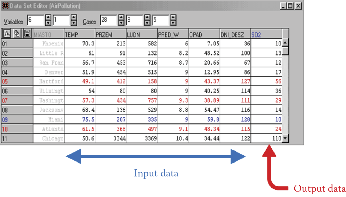
Among the data collected in the database, we can isolate those that will be used as outputs for the network. Look at the range of columns of the table marked by an arrow at the bottom of the figure. The data in the figure should allow us to predict levels of air pollution. The data cover population figures, industrialization levels, weather conditions, and other factors. Based on these data to be used as inputs, the network will have to predict the average level of air pollution in every city.
For a city for which pollution level information has not been compiled, we will have to guess. That is where a network taught earlier will go to work. The learning set data—known pollution data for several cities—has been placed in an appropriate column of the table, which is marked with a red arrow (indicating output data) on Figure 3.1.
Therefore, you have exactly the material you need to teach the network shown in Figure 3.1: a set of data pairs containing the appropriate input and output data. We can see the causes (population, industrialization, and weather conditions) and the result (air pollution value). The network uses these data and will learn how to function properly (guessing the values of air pollution in cities for which proper measurements have not yet been made) via a learning strategy.
Exemplary learning strategies will be thoroughly discussed later. In the meantime, please pay attention to another detail of Figure 3.1. The letters in one column of the table are barely visible because they appear in gray instead of black. This shading suggests that the data portrayed are somewhat less important. The column contains names of particular cities. Based on this information, the database generates new data and results given, but for a neural network the column information is useless. Air pollution has no relationship to the name of a city, so even though these facts are available in the database, we are not going to use them to teach networks. Databases can contain a lot of information data that is not needed to teach a network.
We should remember that the tutor involved in network learning will usually be a collection of data that is not used “as is,” but is adjusted to function as a learning set after cautious selection and proper configuration (data to be used as inputs and data to be generated as outputs). A network should not be littered with data that a user knows or suspects is not useful for finding solutions to a specific problem.
3.2 Self-Learning
Besides the schema of the learning with a tutor described earlier, a series of methods of learning without a teacher (self-learning networks) are also in use. These methods consist of passing only a series of test data to the input of networks, without indicating desirable or even anticipated output signals. It seems that a properly designed neural network can use only observations of entrance signals and build a sensible algorithm of its own activity based on them, most often relying on the fact that classes of repeated (maybe with certain variety) input signals are automatically detected and the network learns (spontaneously, without any open learning) to recognize these typical patterns of signals.
A self-learning network requires a learning set consisting of data provided for input. No output data are provided because in this technique, we need to clarify the expectations from the network analysis of some data. For example, if we apply the data in Figure 3.1 to learning without a teacher, we would use only columns described as input data instead of giving the information from the column noted with the red pointer to the network.
A self-learning network could not have chance to predict in which city the air pollution would be greater or smaller because it cannot gain such knowledge on its own. However, by analyzing the data on covering different cities, the network may favor (with no help) a group of large industrial cities and learn to differentiate them from small country towns that serve as centers of agricultural regions.
The network will develop this distinction from given input data by following a rule that industrial cities are similar and agricultural towns also share many common characteristics. A network can use a similar rule (without help) to separate cities with good and bad weather and determine many other classifications based only on values of observed input data.
Notice that the self-learning network is very interesting from a view of the analogy between such activities of networks and the activities of human brains. People also have abilities to classify encountered objects and phenomena (“formation of notions”) spontaneously. After the execution of the suitable classification, people and networks recognize another object as having characteristics of a previously recognized class.
Self-learning is also very interesting based on its uses. It requires no external knowledge that may be inaccessible or hard to collect. A network will accumulate all necessary information and pieces of news without outside help. Chapter 9 will describe exactly and demonstrate across suitable programs the bases of self-learning of networks.
Now you can imagine (for fun and stimulation of the imagination rather from real need) that a self-learning network with a television camera can be sent in an unmanned space probe to Mars. We are unaware of conditions on Mars. We do not know which objects our probe should recognize or how many classes of objects will appear!
Even without that information, the network will adjust (see Figure 3.2). The probe lands and the network begins the process of self-learning. At first it recognizes nothing and only observes. However, over time, the process of spontaneous self-organization will allow the network to learn to detect and differentiate various types of input signals that appear as inputs: rocks from stones and plant forms from other living organisms. If we give the network sufficient time, it will educate itself to differentiate Martian men from Martian women even though the network creator did not know that Martian people existed!
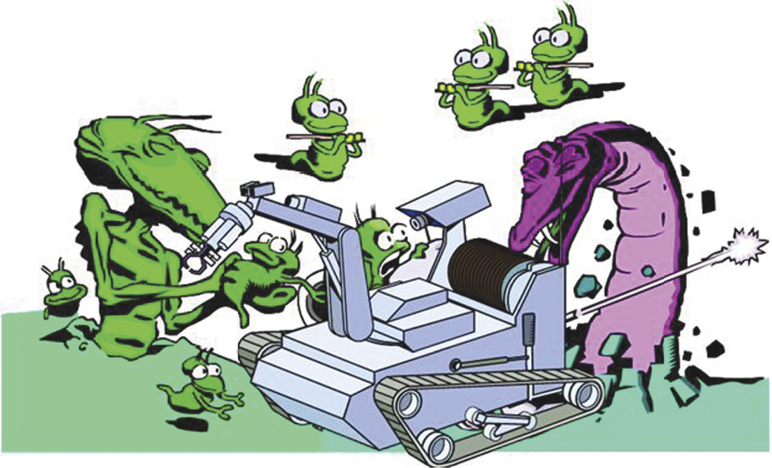
Hypothetical planetary landing module powered with a self-learning neural network can discover unknown (alien) forms of life on mysterious planets.
Of course the self-learning Mars landing vehicle is a hypothetical creation even though networks that form and recognize various patterns exist are in common use. We may be interested in determining how many forms of some little known disease can in fact be found. Is a condition one sickness unit or several? How do the components differ? How can they be cured?
It will be sufficient to show a self-learning neural network the information on registered patients and their symptoms over a long period. The network will later yield information on how many typical groups of symptoms and signs were detected and which criteria can be used to classify patients into different groups. Applications of neural networks to goals like these can lead to a Nobel Prize!
This method of self-learning, of course, has many defects that will be described later. However, self-learning has many undeniable advantages. We should be surprised that the tool is not more popular.
3.3 Methods of Gathering Information
Let us take a closer look at the process of learning with a teacher. How does a network gain and gather knowledge? A key factor is the assignments of weights to each neuron on entrance, as described in Chapter 2.
To review, every neuron has many inputs, by which it receives signals from other neurons and from network data to add its calculations. The parameters called weights are united with the entry data. Every input signal is first multiplied by the weight and only later added to the other signals. If we change values of the weights, a neuron will begin to function within the network in another way and ultimately the entire network will work in another way. The art of learning of a network relies on the choice of weights in such a manner that all neurons will perform the exact tasks the network demands.
A network may contain thousands of neurons and every one of them may handle hundreds of inputs. Thus it is impossible for all these inputs to define the necessary weights simultaneously and without direction. We can, however, design and achieve learning by starting network activities with a certain random set of weights and gradually improving them. In every step of the process of learning, the values of weights from one or several neurons undergo changes. The rules for change are set in such a way that every neuron individual can qualify which of its own weights must change, how (by increase or decrease), and how much.
The teacher passes on the information about the necessary changes of weights that can be used by the neuron. Obviously, what does not change is the fact that the process of changing the weights (as the only memory trace in the network) runs through every neuron of the network spontaneously and independently. In fact, it can occur without direct intervention by the person supervising this process. What is more, the process of the learning of one neuron is independent from how another neuron learns. Thus, learning can occur simultaneously in all neurons of a network (of course only in a suitable network with an adequate electronic system, and not via a simulation program). This characteristic allows us to achieve very high speeds of learning and a surprisingly dynamic increase of qualifications of a network that literally grows wiser and wiser in front of us!
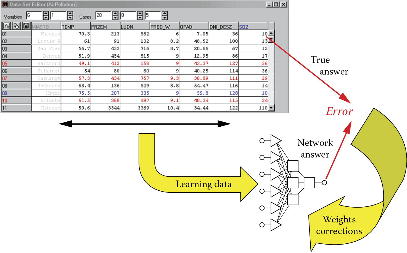
We once again stress a key point: a teacher need not get into the details of the process of learning. It is sufficient for the teacher to give a network an example of a correct solution. The network will compare its own solution obtained from the example originating from the learning set with the solution that was recorded in the learning set as a model (most probably correct). Algorithms of learning are constructed so that the knowledge about the value of an error is sufficient to allow a network to correct values of its weights. Every neuron separately corrects its own weights on all entries under the control of the specific algorithm after it receives an error message.
Figure 3.3 depicts a very simple but efficient mechanism. Its systematic use causes the network to perfect its own activities until it is able to solve all assignments from the learning set and on the grounds of generalization of this knowledge. It can also handle assignments that will be introduced to it at the examination stage.
The manner of network learning described earlier is used most often, but some assignments (e.g., image recognition) do not require a network to have the exact value of a desired output signal. For efficient learning, it is sufficient to give a network only general information on a subject, whether its current behavior is correct, or not. At times, network experts speak about “rewards” and “punishments” in relation to the way all neurons in a network find and introduce proper corrections to their own activities without outside direction. This analogy to the training of animals is not accidental.
3.4 Organizing Network Learning
Necessary changes of values of weight coefficients in each neuron are counted according to special rules (sometimes called paradigms of networks). The numbers of different rules that are used today and their varieties are extreme because most researchers try to demonstrate their own contributions to the field of neural networks as new rules of learning.
We now consider two basic rules of learning without using mathematics: (1) the rule of the quickest fall lying at the bases of most algorithms of learning with a teacher and (2) the Hebb rule defining the simplest example of learning without a teacher (see Section 3.10).
The rule of the quickest fall relies on the receipt by every neuron of definite signals from the network or from other neurons. The signals result from earlier levels of processing the information. A neuron generates its own output signal using its knowledge of earlier settled values of all amplification factors (weights) of all entries and (possibly) the threshold.
Methods of marking the values of output signals by neurons based on input signals were discussed in detail in Chapter 2. The value of the output signal of a neuron at each step of the process of learning is compared with the standard answer of the teacher within the learning set.
In the case of divergence that will appear almost certainly at the initial stage of the learning process, the neuron finds the difference between its own output signal and the value of the signal the teacher indicates is correct. The neuron then (by the method of the quickest fall to be described shortly) decides how to change the values of the weights to decrease the error.
It is useful to understand the area of an error. You already know that the activity of a network relies on the values of weight coefficients of the constituent neurons. If you know the set of all weight coefficients appearing in all neurons of the entire network, you know how such a network will act. Particularly you can show a network all examples of assignments and solutions accessible as part of the learning set. Every time the network produces its own answer to an asked question, you can compare its answer to the pattern of the correct answer found in the learning set, thus revealing the network error.
A measure of this error is usually the difference between the value of the result delivered by the network and the value of the result read from the learning set. To rate the overall activities of networks with defined sets of weight coefficients in their neurons, we usually use the pattern of the sum of squares of errors committed by the network for each case from the learning set. The errors are squared before summing to avoid the effect of mutual compensation of positive and negative errors. This results in heavy penalties for large errors. A twice greater error is a quadruple component in the resulting sum.
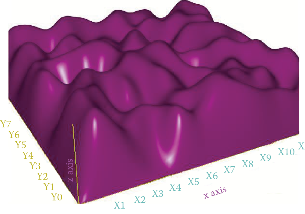
Note in Figure 3.4 the yellow (lighter tone) rectangle and cloud first, then the green (darker tone) rectangle and cloud. The figure depicts a situation that could occur in a network so small that it would have only two coefficients of weights. Such small neural networks do not exist, but let us assume that you have such a very small network. We will attempt to analyze its behavior without getting into difficulties arising from multidimensional spaces. Every state of good or poor learning of this network will be joined at some point on the horizontal (light blue) visible surface shown in the figure with its weight coefficient coordinates. Imagine now that you placed weight values in the network that comply with the location of the red point on the surface. Examining such a network by means of all elements of the learning set will reveal the total value of the error. In place of the red point you will put a red arrow pointing up. The height will represent the calculated value of the error according to the vertical axis in the figure.
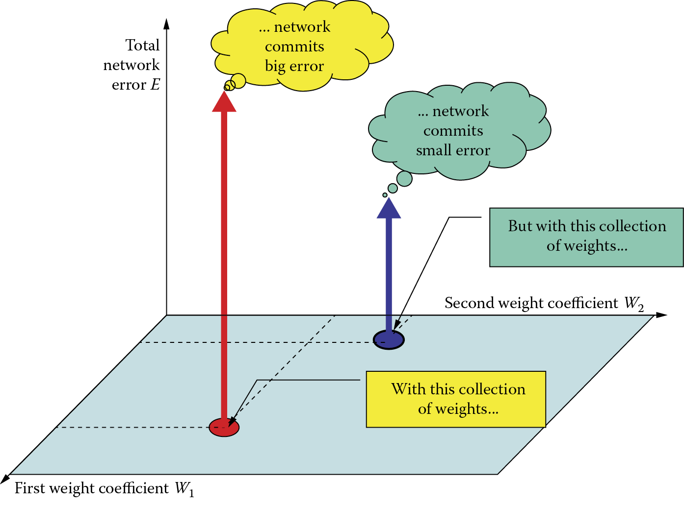
Next, choose other values of weights, marking their positions on the surface (navy blue) and perform the same steps utilizing the navy blue pointer. Imagine that you perform these acts for all combinations of weight coefficients, that is, for all points of the light blue surface. Some errors will be greater and other smaller. If you had the patience to examine your network many times, you would see the error surface spread over the surface of the changed weights.
You can see many “knolls” on the surface in Figure 3.5. These indicate where the network committed several errors and should be avoided. The neural network committed smaller errors as shown by the deep valleys. This indicates the network solves its tasks especially well, but how do we find the valleys?
The learning of a neural network is a multistage-process. Each step of the process is intended to improve values of weights in the network, changing unsatisfactory sets of weights that may cause large errors for new weights that hopefully will perform better (see Figure 3.6).
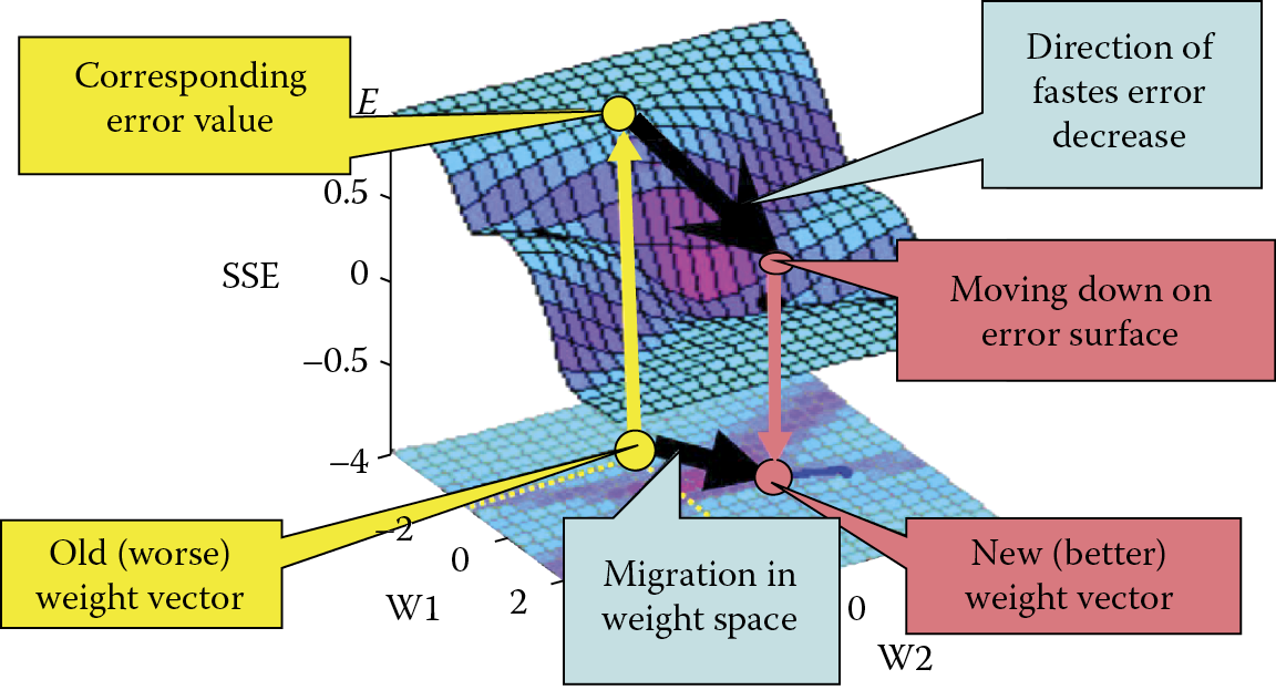
Starting at the bottom left corner of the figure, we see an old (vector) set of weights, noted on the parameter surface of the network with a yellow (light tone) circle. For this vector of weights, you find the error and “land” on the surface of the error shown with a yellow arrow in the left upper corner of the figure. The error rate is very high and the network temporarily has incorrect parameters. It is necessary to improve this situation, but how?
A neural network can be taught to find a way to change the weight coefficients to decrease error rates. The direction of the quickest fall of the error is noted in Figure 3.6 as a large black pointer. Unfortunately, the details of the learning method cannot be explained without using complicated mathematics and such notions as the gradient and partial derivative. However, the conclusions yielded by these complex mathematical considerations are simple enough. Every neuron in a network modifies its own weight and possibly threshold coefficients using two simple rules:
- Weights are changed more strongly when great errors are detected.
- Weights connected on which large values of input signals appeared are changed more than weights on which input signals were small.
The basic rules may need additional corrections even though the outline of the method of learning is understood. Recognizing an error committed by a neuron and knowing its input signals allow a designer to foresee easily how its weights will change. The mathematics-based rules are very logical and sensible. For example, the faultless reaction of a neuron to a specific input signal should proceed without a change if its weights are correctly calculated.
A network using prescribed methods in practice breaks the process of learning when it is well trained. Small errors require only minimum cosmetic corrections of weights. It is logical to subordinate the size of a correction based on the size of the input signal delivered. Inputs that have greater signals exert more influence on the result of the activity of a neuron. To ensure a neuron operates correctly, it must be “sharpened.”
We now return to the process of learning shown in Figure 3.6. After we find the direction of the quickest fall of the error, the algorithm of learning the network makes a change in the weight space and replaces the incorrect vector with a correct one. The migration causes the error to “slide down” to a new point, usually lower, to approach the valley where errors are the fewest and eventually solve assignments perfectly. This optimistic scenario of gradual and efficient migration to the area where errors are minimal is shown in Figure 3.7.
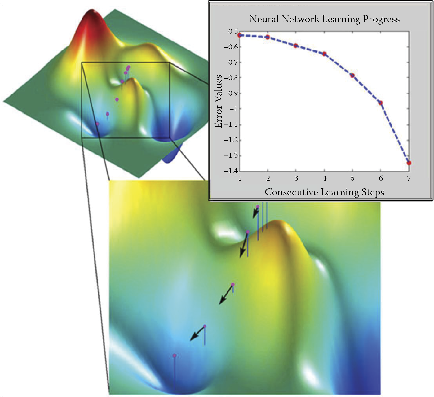
Searching for and finding network parameters (weight coefficients for all neurons) guaranteeing minimal error values during supervised learning.
3.5 Learning Failures
Learning is not always a simple and pleasant process as depicted in Figure 3.7. At times, a network “struggles” until it finds a suitable solution. A detailed discussion of difficulties arising from learning would require complicated considerations of differential calculus and analysis of the convergence of algorithms. We will try to explain learning problems without detailing complicated mathematics by telling a story about a blind kangaroo (Figure 3.8).
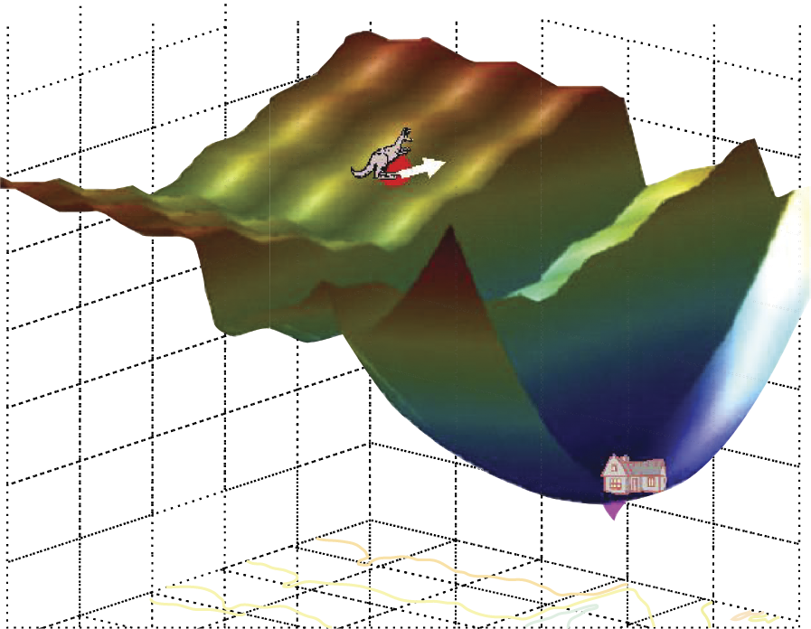
Imagine a blind kangaroo is lost in the mountains and wants to return to his home. The kangaroo knows only one fact about the location of his house: it is situated at the very bottom of the deepest valley. The kangaroo cannot see the surrounding mountain landscape just as an algorithm of learning cannot check the values of the error functions at all points for all sets of weights.
The kangaroo can only use his paws to feel which way the ground subsides in the same way a network learning algorithm can determine how to change weights to make fewer errors. The kangaroo thinks he has found the correct direction and hops with all his power, thinking that the hop will deliver him to his home.
Unfortunately a few surprises await the kangaroo and the algorithm for teaching a neural network. Note from Figure 3.8 that an incorrectly aimed jump can lead the kangaroo into a rift that separates him from his house. Another situation not shown in the figure but easy to imagine is that the ground in what appears a promising direction can drop and then suddenly elevate. As a result, the kangaroo’s long jump in that direction will make his situation worse, because he will find himself landing higher (farther from the low valley where he lives) than he was at the start of his quest.
The success of the poor little kangaroo depends mostly on whether he can properly measure the length of the jump. If he is too cautious and performs only small jumps, his journey home will take longer. If he jumps too far and the surrounding area has cliffs and rifts, he may be injured.
As a network learns, the creator of the algorithm must decide the sizes of weight changes based on specific values of input signals and the potential sizes of errors. The decision is made by changing the so-called proportion coefficient or learning rate. Apparently, the algorithm designer has a great number of choices but every decision generates specific consequences.
Choosing a coefficient that is too small makes the process of learning very slow. Weights are improved very slightly at every step. Thus many steps must be performed for the network to reach desirable values. Choosing a too large coefficient of learning may cause abrupt changes to the parameters of the network; in extreme cases, this can cause learning instability, as a result of which the network will be unable to find the correct values of weights. Changes made too quickly will make it difficult for a network to reach the necessary solution.
We can view this problem from another point. Large values of the coefficient of learning resemble the attitude of a teacher who is very strict and difficult to please and severely punishes pupils for their mistakes. Such a teacher seldom attains good learning results because he creates confusion and imposes excessive stress on his students. On the other hand, low values of a coefficient of learning resemble a teacher who is excessively tolerant. Her pupils progress too slowly because she fails to motivate them to work.
In the processes of teaching networks and teaching pupils, compromises are necessary. Teaching means balancing the advantages of quick results with safety considerations to achieve stable functioning of the process of learning. A method to accomplish this goal is described in the next section.
3.6 Use of Momentum
One way of increasing the learning speed without interfering with stability is using an additional component called momentum in the algorithm of learning. Momentum enlarges the process of learning by changing the weights on which the process depends and the current errors, and allows learning at an earlier stage.
Figure 3.9 allows a comparison of learning with and without momentum and the process of changing the weight coefficients. We can show only two of them, and thus the drawing should be interpreted as a projection on plane determined by weight coefficient wi and the weight adaptation process wj that takes place in the n dimensional space of the weights. We can see behavior of only two inputs for a specific neuron of the network, but the processes in other neurons are similar.
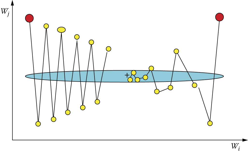
Red (dark tone) points represent starting points (the setting before the start of learning the values of weight coefficients). Yellow points indicate the values of weight coefficients obtained during the steps of learning. An assumption has been made that the minimum of the error function is attained at the point indicated by the plus sign (+). The blue ellipse shows the outline of the stable error (set of values of weight coefficients for which the process of learning attains the same level of error).
As shown in the figure, introducing momentum stabilizes the learning process as the weight coefficients do not change as violently or as often. This also makes the process more efficient as the consecutive points approach the positive point faster. We use momentum for learning from a rule because it improves the attainment of correct solutions and the execution costs are lower.
Other manners of improving learning can involve changing the values of the coefficients of learning—small at the beginning of the process when the network chooses the direction of its activity, greater in the middle of learning when the network must act forcefully to adapt the values of its parameters to the rules established for its activity, and finally smaller at the end of learning when the network fine-tunes the final values of its parameters and sudden corrections can destroy the learning structure. The techniques resemble the elaborate methods of a human teacher who has a large body of knowledge to use to train pupils with limited abilities.
Every creator of an algorithm of learning for a neural network faces the problem of assigning original values of coefficients of weights. The algorithm of learning described earlier shows how we can improve the values of these coefficients during learning. At the instant of onset of learning, the network must have concrete values of coefficients of the weights to be able to qualify the values of output signals of all neurons and to compare them to values given by the teacher for the purpose of qualification of errors. Where should we get these original values?
The theory of the learning process says that at the realization of certain (simple) conditions, a linear network can learn and find correct values of weight coefficients based on initial values we set at the start of the learning process. In the domain of non-linear networks, the situation is not so simple, because the process of learning can “get stuck” in the starting values of the so-called minima of local error functions. In effect, this means that starting from different primary sets of weight coefficients can yield different parameters of the taught network—appropriate or incorrect for resolving the set assignment.
What does the theory say about choosing correct starting points? Here we must support our knowledge with empiricism. A common practice relies on the fact that the primary values of weight coefficients are random. At the beginning, all parameters receive accidental values, so we start from a random situation. This may sound strange but actually makes sense. Because we know where to find minimum error functions, there is no better solution than relying on randomness.
Simulator programs contain special instructions for “sowing” the first random values of coefficients in a network. We should avoid excessively large values of start coefficients. Normal practice is to choose random values from the area between –0.1 and +0.1. Additionally, in many-layered networks, we must avoid coefficients having 0 values because they block the learning process in deeper layers. Weight signals do not pass through 0 values of weights. The result is cutting off part of the network structure from further learning.
Of course, the progress of learning reduces error potential. Learning is rapid at the beginning, then slows somewhat, and finally stops after completion of certain steps. It is useful to remember that learning by targeting training of the same assignment by means of the same network can run differently. Figure 3.10 shows three courses of this process that differ by the speed of progress of learning final effects. The difference results from the size of the coefficient of the error, below which a network cannot operate despite the intensity of further learning. The graphs refer to the same network and the same assignment and differ only in the primary values of coefficients of weights. We can thus say that they show diverse “inborn abilities” of the network.
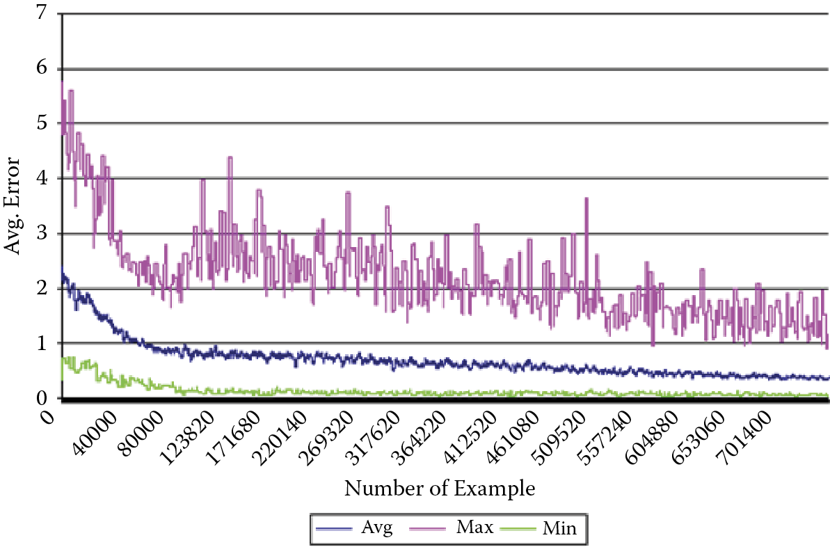
The neural network learned many times using the same learning set, but starting from different points (determined by random setting of initial weight values). Three courses are plotted: average (most representative), course with maximal end value of post-learning error (pessimistic case), and course with minimal end value of post-learning error (optimistic case). In some networks, (e.g., Kohonen types) an additional learning demand is that original values of weight coefficients be normalized. We will talk about this in Chapter 10.
3.8 Duration of Learning Process
Unfortunately, the answer to determining duration of learning is pessimistic. The simplicity of training a network instead of the complex process of programming it extracts a price: a long period of learning. We currently accept the price because no one has found an efficient way to shorten network learning processes. Furthermore, it is difficult to anticipate the time it will take to teach a network until it begins to develop some elements of intelligent behavior. Sometimes the process is speedy but generally it is necessary to use the elements of a learning set for a long time and with great effort before a network begins to understand some of its task.
What is more, as the result of random choice of original values of weight coefficients, the learning results for the same data used as the learning set can differ a little and this fact should be accepted unless a designer time to teach the same network several times and choose the variant that guarantees the best result. A single process of learning for a network with several thousands of elements lasts several hours! For example, a neural network designed for face recognition built from 65,678 neurons in a three layer perceptron structure needs 5 hours and 23 minutes of learning time using a Dell PC with 1.2 GHz clock. The learning set contains 1,024 example images of 128 known persons (8 images per person).
The long learning process is not an isolated result. For example, a compilation published in the Electronic Design monthly lists the numbers of presentations of the learning set required to achieve certain tasks as shown in the table below. Other authors noted similar results.
|
Function |
Number of Presentations |
|
Kanji character recognition |
1013 |
|
Speech recognition |
1012 |
|
Recognition of manuscript |
1012 |
|
Voice synthesis |
1010 |
|
Financial prediction |
109 |
|
Source: Wong, W. Neural net chip enables recognition for micro. Electric Design, June 22, 2011. |
|
Because of the learning time required, researchers seek methods other than the classical or delta algorithms for teaching networks. The time of teaching a network with the algorithm of the quickest fall (described earlier) grows exponentially as the number of elements increases. This fact limits the sizes of neural networks.
3.9 Teaching Hidden Layers
Finally, we will discuss the teaching of hidden layers of networks. As described in Chapter 2, all layers of a network other than the entrance (input) and exit (output) layers are hidden. The essence of the problem of teaching neurons of the hidden layer arises because we cannot directly set the sizes of errors for those neurons because the teacher provides standard values of signals only for the exit layer. The teacher has no basis for comparison for signals from neurons of the hidden layer.
One solution to this problem is backward propagation (backpropagation) of errors suggested by Paul Werbos and later popularized by David Rumelhart whose name is usually connected to the method. Backpropagation consists of reproducing the presumable values of errors of deeper (hidden) layers of network on the ground of projecting backward the errors detected in the exit layer. The process will be detailed in Chapter 7.
Basically, the technique considers the neurons to which the hidden layer sends output signals and adds the signals, taking into account the values of coefficients of weights of connections between hidden layer neurons and neurons that produced errors. This way the “responsibility” for errors of neurons of the hidden layer burdens those neurons more heavily (with greater weight) because they influence the signals transmitted to the exit layer. By proceeding backward in this manner from the exit neurons to the entry neurons of a network, we can evaluate presumable errors of all neurons and consequently gain sufficient information to make the necessary corrections of weight coefficients of these neurons.
Of course, this method does not allow us to mark errors of neurons of intermediate layers exactly. As a result, corrections of errors during the learning process are less accurate than corrections made in networks without hidden layers. Finding and correcting errors with this technique adds to network learning time. However, the wide range of capabilities of networks with multiple layers means we must accept the tens of thousands of demonstrations involved in a learning set.
Other problems may arise through the repeated presentation of a learning set to a network. The necessary repetition would try the patience of a human teacher who could never deal with the hundreds of thousands or millions of operations required to teach a neural network. At present we have no alternative for presenting the same input signals and patterns to a network as many times as it needs to learn answers.
It is detrimental to show learning set elements always in the same order. Such predictable instruction can allow a network to establish definite cycles of values of weight coefficients and will halt the process of learning and possibly cause network failures. It is vital to randomize the learning process by mixing the elements and presenting them in different orders. The randomization complicates learning but it is crucial for obtaining reasonable results.
3.10 Learning without Teachers
How is it possible to learn without a teacher? We know that a network should be capable of resolving a specific task without having a set of ready examples with solutions. Is this possible? How can we expect a network to perfect its own work without receiving instructions?
In practice, it is entirely possible and even relatively easy to teach a spontaneous self-organizing neural network subject to a number of simple conditions. The simplest idea of self-learning of a network is based on the observations of Donald Hebb, a US physiologist and psychologist. According to Hebb, the processes of strengthening (amplification) of connections between neurons occur in the brains of animals if the connections are stimulated to work simultaneously. The associations created in this manner shape reflexes and allow simple forms of motor and perceptive skills to develop.
To transfer Hebb’s theories to neural network operation, computer scientists designed a method of self-learning based on showing a network examples of input signals without telling the network what to do with them. The network simply observes the signals in its environment although it is not told what the signals mean or what relationships exist between them. After observing the signals, a network gradually discovers their meaning and sets dependencies among the signals. The network not only acquires knowledge, but in a way creates it! Let us now discuss this interesting process in more detail.
After processing consecutive sets of input signals, a network forms a certain distribution of output signals. Some neurons are stimulated very intensely, others weakly, and some even generate negative signals. The interpretation of these behaviors is that some neurons “recognize” signals as their own (are likely to accept them), others are indifferent to the signals, while other neurons are simply “disgusted” by them. After the production of output signals of all neurons throughout a network, all weights of the input and output signals are changed. It is easy to see that this is a version of the Hebb postulate in that connections between sources of strong signals are noted and strengthened.
Further analysis of the process of self-learning based on the Hebb method allows us to state that after consistent use of a specific algorithm for start parameters, neurons develop accidental “preferences” that lead to systematic strengthening and detailed polarization. If a neuron has an “inborn inclination” to accept certain types of signals, it will learn after repetition to recognize these signals accurately and precisely. After a long period of such self-learning, the network will create patterns of input signals spontaneously.
As a result, similar signals will be recognized and assembled efficiently by certain neurons. Other types of signals may become “objects of interest” to other neurons. Through this process of self-learning, a network will learn without a teacher to recognize classes of similar input signals and assign the neurons that will differentiate, recognize, and generate appropriate output signals. So little to accomplish so much!
3.11 Cautions Surrounding Self-Learning
The self-learning process unfortunately displays many faults. Self-learning takes much longer than learning with a teacher. For this reason, a controlled process is preferable to spontaneous learning. Without a teacher, we never know which neurons will specialize in diagnosing which classes of signals. For example, one neuron may stubbornly recognize the letter R, another may recognize Ds, and a third may see Gs. No learning technique can make these neurons arrange themselves in alphabetical order.
This creates a certain difficulty when interpreting and using the output of a network, for example, to steer a robot. The difficulty is basic but it may produce troublesome results. We have no guarantee that neurons developing their own random starting preferences will specialize to the extent that they will process different classes of entrance images. It is very probable that several neurons will “insist” on recognizing the same class of signals, for example As, and no neurons will recognize Bs.
That is why a network intended to be self-learning requires more effort than a network solving the same problem with the participation of a teacher. It is difficult to measure the difference exactly. Our past experiments indicate that a network intended to be self-learning must have at least three times as many elements (especially in the exit layer) than the answers it is expected to generate after learning.
A very subtle and essential matter is the choice of the starting weight values for neurons intended to be self-taught. These values strongly influence the final behavior of a network. The learning process deepens and perfects certain tendencies present from the beginning of the process. Thus these innate properties of a network strongly affect the end processes of learning.
Without knowing from the beginning which assignment a network should learn, it is difficult to introduce a specific mechanism to set the start values of weights. However, leaving these decisions to random mechanisms can prevent a network (especially a small one) from sufficiently diversifying its own mechanisms at the start of learning. Subsequent efforts to represent entrance signals of all classes in the structure of a network may prove futile.
However, we can introduce one mechanism for initial distribution of the values of weights in the first phase of learning. This method, known as convex combination, modifies original values of the weights in a way that maximizes the probability of an even distribution of all typical situations appearing in the entrance data set among neurons. If data appearing in the first phase of the learning will not differ from data to be analyzed and differentiated by a network, convex combination will create a convenient starting point to further self-learning automatically and also ensure relatively good quality of solutions to assignments.
Questions and Self-Study Tasks
1. What conditions must be fulfilled by a data set to allow it to be used as a teaching set for a neural network?
2. How does teaching a network with a teacher differ from teaching without a teacher?
3. On what grounds does the algorithm of teaching calculate the directions and changes of weights in the steps of teaching?
4. How should we set the starting values of weight coefficients of a network to start its learning process?
5. When does the teaching process stop automatically?
6. Why do network teaching efforts fail and how can we prevent failures?
7. Describe the steps of generalizing knowledge obtained by a neural network during teaching.
8. Where can we obtain the data necessary to fix the values of changes of weight coefficients of neurons in hidden layers during teaching?
9. What is momentum and what can we do with its help?
10. How much time is required to teach a large network? What factors determine the time required?
11. Why do we speak about “discovering knowledge” of self-learning networks instead of “teaching” them?
12. Advanced exercise: Suggest a rule that allows us to change the coefficient of teaching (learning rate) in a manner that will accelerate the speed of learning in safe situations and slow it at the moment when the stability of the teaching process is endangered. Note: Consider changes of the valued of errors committed by a network in subsequent steps of teaching.