Chapter 4

Functioning of Simplest Networks

4.1 From Theory to Practice: Using Neural Networks

The intent of the previous chapters was to provide a theoretical basis of neural network design and operation. Starting with this chapter, readers will gain practice in using neural networks. We will use simple programs to illustrate how neural networks work and describe the basic rules for using them. These programs (along with data required for start-up) can be found at http://www.agh.edu.pl/tad* on the Internet.

This address will lead you to a site that accurately describes step by step all the required actions for using these programs legally and at no cost. You need these programs to verify information about neural networks contained in this book. Installing these programs in your computer will enable you to discover various features of neural networks, conduct interesting experiments, and even have fun with them.

Don’t worry. Minimal program installation experience is required. Detailed installation instructions appear on the website. Note that updates of the software will quickly make the details in this book outdated. Despite that possibility, we should explain some of the procedures.

Downloading the programs from the site is very easy and can be done with one mouse click. However, obtaining the programs is not enough. They are written in C# language and need installed libraries in .NET Framework (V. 2.0). All the needed installation software is on the site.

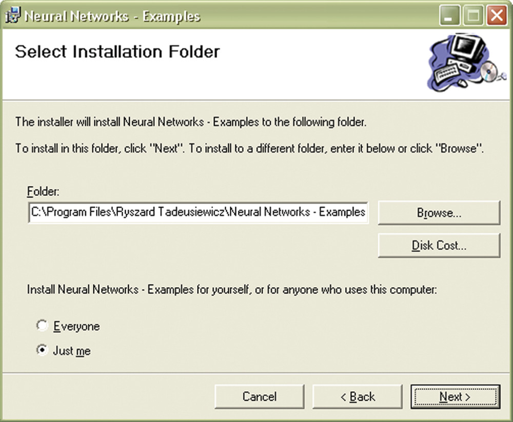
The first step is the installation of the libraries (Figure 4.1). You may have some of these libraries installed on your computer already and conclude that this step is unnecessary. If you are certain about that, you can skip the .NET Framework step, but we suggest you perform it “just in case.”

If the appropriate programs are installed on your computer already, the install component will determine that it has no need to install them. However, the site may contain newer versions of the libraries than the ones you have, in which case the installer will go to work. It is always smart to replace old software with newer versions. The new software will serve many purposes beyond those described in this book.

After you install the necessary .NET Framework libraries on which further actions depend according to the site guidelines, the installer will run again. This will allow you to install all example programs automatically and painlessly. You will need them for performing experiments covered in this book. When the installation is finished, you will be able to access the programs via the start menu used for most programs. Performing .NET experiments will help you understand neural networks theoretically and demonstrate their use for practical purposes.

To convince unbelievers that this step is simple, Figure 4.1 shows the difficult part of installation: the installer asks the user (1) where to install the programs and (2) who should have access. The best response is to keep the default values and click on Next. More inquisitive users have two other options: (1) downloading the source code and (2) installing the integrated development environment called Visual Studio.NET.

The first option allows you to download to your computer hard drive the text versions of all the sample programs whose executable versions you will use while studying this book. It is very interesting to check how these programs are designed and why they work as they do. Having the source code will allow you—if you dare—to modify the programs and perform even more interesting experiments. We must emphasize that the source codes are not necessary if you simply want to use the programs. Obviously, having codes will enable you to learn more and use the resources in more interesting ways. Obtaining the codes is not a laborious process.

The second option, installing Visual Studio.NET, is addressed to ambitious readers who want to modify our programs, design their own experiments, or write their own programs. We encourage readers to install Visual Studio.NET even if they only want to view the code. It is worthwhile to spend a few more minutes to make viewing of the code easier. Visual Studio.NET is very easy to install and use. After installation, you will be able to perform many more actions such as adding extern sets, diagnosing applications easily, and quickly generating complicated versions of the software.

Remember that the installations of source codes and Visual Studio.NET are totally optional. To run the example programs that will allow you to create and test neural network experiments described in this book, you need only install .NET Framework (first step) and example programs (second step).

What’s next? To run any example, you first choose an appropriate command from the Start/Programs/Neural Networks Examples menu. After making your selection, you may use your computer to create and analyze every neural network described in this book. Initially your system will use a network whose shape and measurements we designed. After you are immersed in the source code, you will be able to modify and change whatever you want. The initial program will make networks live on your computer and allow you to teach, test, analyze, summarize, and examine them. This manner of discovering the features of the neural networks—by building and making them work—may be far more fulfilling than learning theory and attending lectures.

The way a network works depends on its structure and purpose. That is why we will discuss specific situations in subsequent chapters. Because the simplest network function to explain is image recognition, we will start our discussion there. This type of network receives an image as an input and after categorization of the image based on previous learning, it produces an output. This kind of network was presented in Figure 2.39 in Chapter 2. A network handles the task of classifying geometric figures by identifying printed and handwritten letters, planes, silhouettes, or human faces.

How does this type of network operate? To answer that, we start from an absolutely simplified network that contains only one neuron. What? You say that a single neuron does not constitute a network because a network should contain many neurons connected to each other? The number of neurons does not matter and even so small a network can produce interesting outputs.

4.2 Capacity of Single Neuron

As noted earlier, a neuron receives input signals, multiplies them by factors (weights assigned individually during the learning process) that are summed and converge to a single output signal. To review, you know already that summed signals in more complicated networks converge to yield an output signal with an appropriate function (generally nonlinear). The behavior of our simplified linear neuron involves far less activity.

The value of the output signal depends on the level of acceptance between the signals of every input and the values of their weights. This rule applies ideally only to normalized input signals and weights. Without specific normalization, the value of an output signal may be treated as the measure of similarity between assembly of the input signals and the assembly of their corresponding weights.

You can say that a neuron has its own memory and stores representations of its knowledge (patterns of input data as values of the weights) there. If the input signals match the remembered pattern, a neuron recognizes them as familiar and answers them with a strong output signal. If the network senses no connection between the input signals and the pattern, the output signal is near 0 (no recognition). It is possible for a total contradiction to occur between the input signals and weight values. A linear neuron generates a negative output signal in that case. The greater the contradiction between the neuron’s image of the output signal and its real value, the stronger its negative output.

We encourage you to install and run a simple program named Example 01a to perform a few experiments. You will learn even more about networks if you try to improve the program. After initializing Example 01a, you will see the window in Figure 4.2. The text in the top section explains what we are going to do.

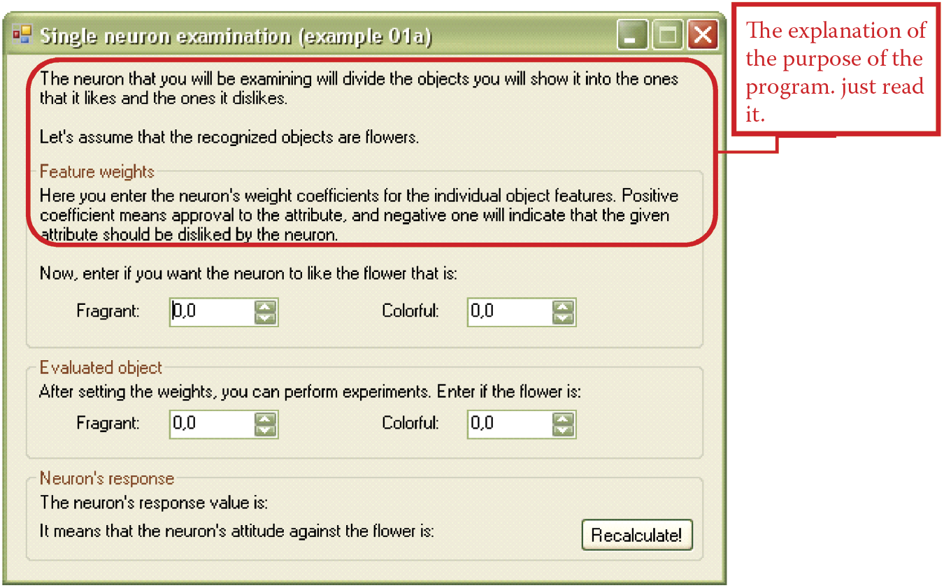
The blinking cursor signals that the program concerning flower characteristics is waiting for the weight of the neuron’s input (in this case the fragrant value). You can enter the value by typing a number, clicking the arrows next to the field, or using the up and down arrows on the keyboard. After inserting the value for the fragrant feature, go on to the next field that corresponds to the second feature—color.

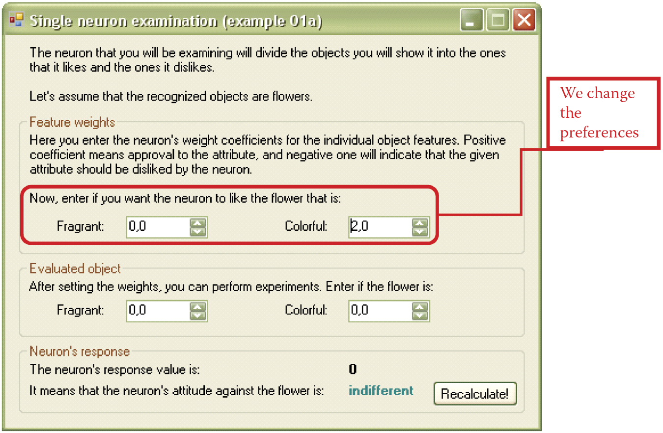
Let us assume that you want your neuron to like colorful and fragrant flowers, with more weight for color. After receiving an appropriate answer, the window of the program will resemble Figure 4.3.

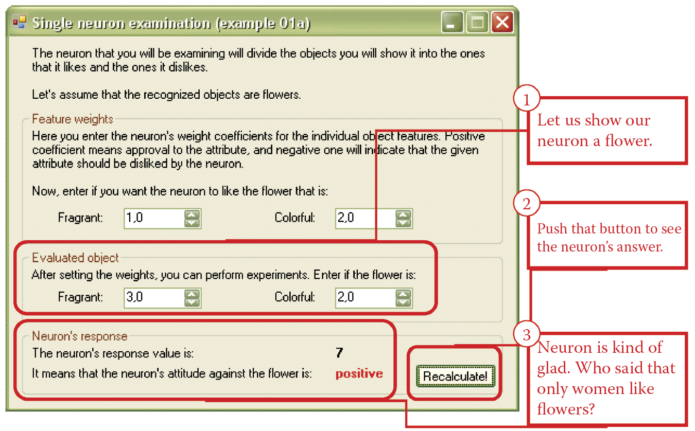
This program and every other one you will use allows you to change your decision and choose another input. The program will try to update the results of its calculations. After we input the feature data (which in fact are weight values), we can study how the neuron works. You can input various sets of data as shown in Figure 4.4 and the program will compute the resulting output signal and its meaning. Remember that you can change the neuron’s preferences and the flower description at any time.

If you use a mouse or arrow keys to input data, you do not have to click the recalculate button every time you want to see the result; calculations are made automatically. When you input a number from the keyboard, you have to click the button because the computer does not know whether you finished entering the number or left to get a tuna sandwich.

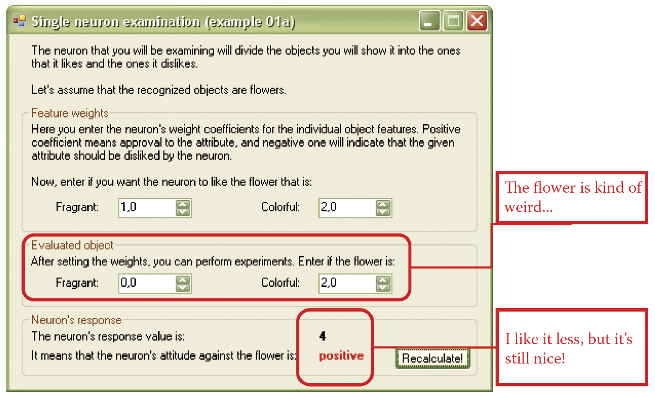
The next stage is to experiment with a neuron in an unusual situation. The point of the experiment shown in Figure 4.5 is to observe how the neuron reacts to an object that differs from its remembered ideal colorful and fragrant flower. We showed the neuron a flower full of colors with no fragrance. As you can see, the neuron liked this flower as well!

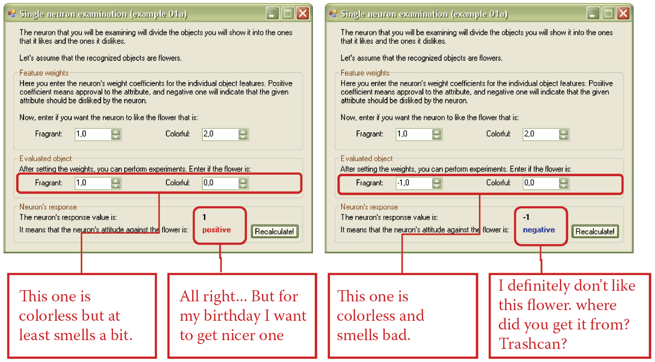
Changing the parameters of the flower allows us to observe what the neuron will do in other circumstances. The examples of such experiments are shown in Figure 4.6 and Figure 4.7. We tested the behavior of the neuron when the flower had a pleasing fragrance and little color. The network liked it anyway. We then tested a colorless flower with an unpleasant smell; that one was not likeable.

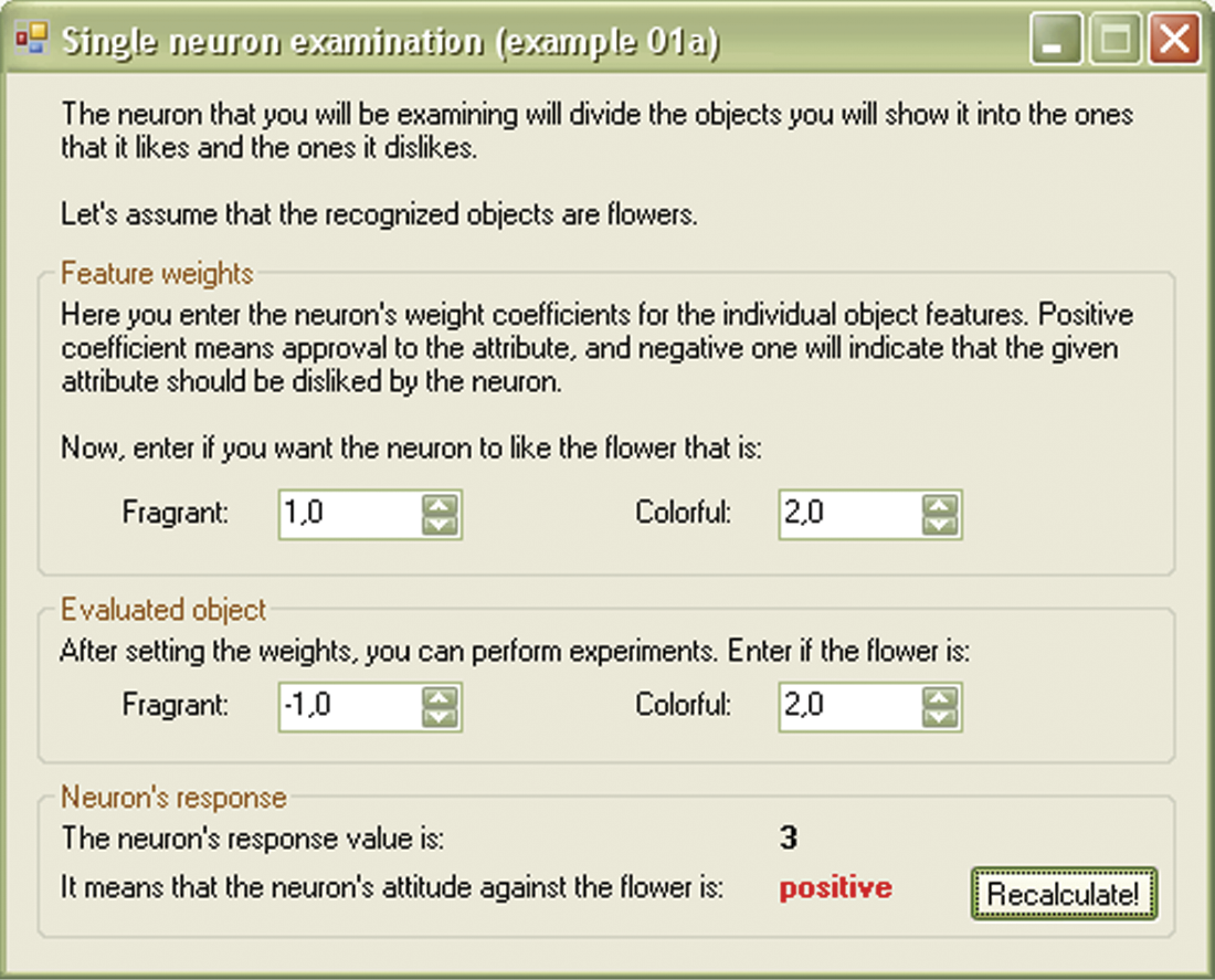
Now let us test our neuron with a little more complicated task: whether it accepts a flower that smells badly if it is colorful enough. As you can see, the program provides plenty of ways to experiment. You can change the preferences of the neuron to see how it reacts in various situations, for example, it may like a flower that smells bad (the weight for fragrance can be negative).

4.3 Experimental Observations

You will find “playing” with the Example 01a program a worthwhile exercise. As you input various data sets, you will quickly see how a neuron works according to a simple rule. The neuron treats its weight as a model for the input signal it wants to recognize. When it receives a combination of signals that corresponds to the weight, the neuron “finds” something familiar and reacts enthusiastically by generating a strong output signal. A neuron can signal indifference by a low output signal and even indicate aversion via a negative output because its nature is to react positively to a signal it recognizes.

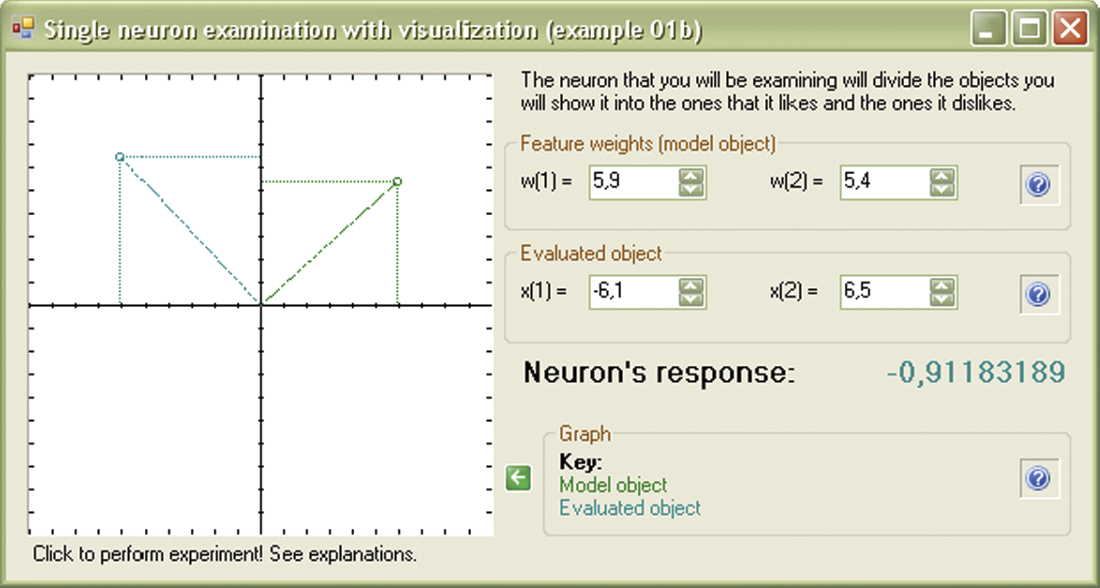
Careful examination will indicate that the behavior of a neuron depends only on the angle between the vector of weight and the vector of the input signal. We will use Example 01b to further demonstrate a neuron’s likes and dislikes by presenting an ideal flower as a point (or vector) in input space.

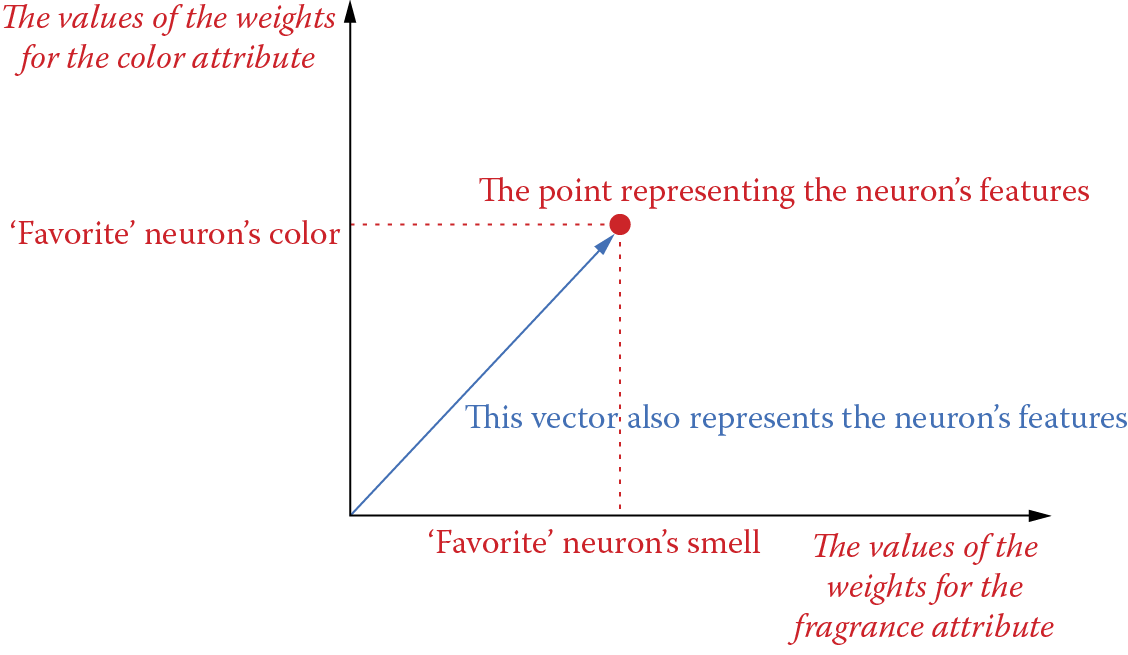
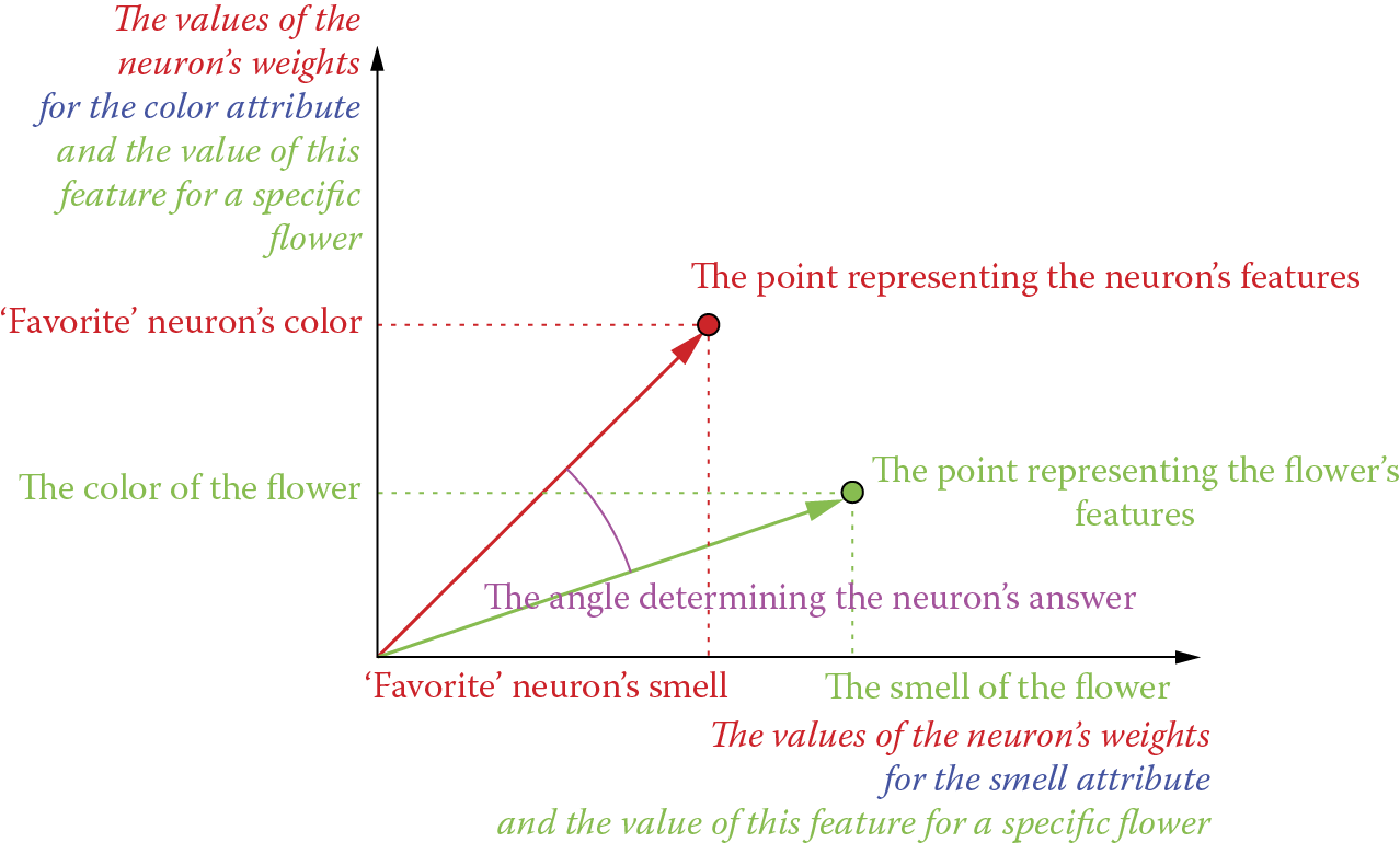
When you set the preferences of a neuron, you tell it, for example, to like fragrant and colorful flowers. Fragrance and color are separate weight vectors. You can draw two axes. On the horizontal axis, you can note the values of the first feature (fragrance) and indicate the values of the second feature (color) on the vertical axis (Figure 4.8). You can mark the preferences of the neuron on the axes. The point created where these coordinates meet indicates the neuron’s preferences.

A neuron that values only the fragrance of a flower and is indifferent to color will be represented by a point located maximally to the right (high value of first coordinate) but on the horizontal axis set at a low number or zero. A puttyroot flower has beautiful colors and a weak and sometimes unpleasant smell. The puttyroot would be located high on the vertical axis (high color value) and to the left of this axis to indicate unpleasant or weak smell. Flower color is valued on the vertical axis and fragrance on the horizontal axis. You can treat any object you want a neuron to mark by using this technique.

A lily of the valley has a wonderful smell and would be represented by the point located maximally to the right. However, its color is not a strong asset so color would be valued low on the axis. The beautiful and unpleasant smelling gillyflower would be rated high on the color axis and low on the fragrance side. The sundew would appear at the bottom left segment of the system; it looks like rotting meat and has a similar smell intended to attract insects. Majestic and fragrant roses would be valued at the top right corner.

On a neural network, it is convenient to mark objects (ideal flowers and flowers to be analyzed) as points on a coordinate system and as vectors. You can acquire needed vectors by joining the points with the beginning of the coordinate system. This is how Example 01b works. Similar to Example 01a, it can be found in on the start menu. Certain features should be noted:

• The value of the output depends mostly on the angle between the input vector (representing input signals) and the weight vector (ideal object accepted by the neuron). It is illustrated in Figure 4.9.
• If the angle between the input and weight vectors is small (the vectors are located next to each other), the value of neuron output is positive and high.
• If the angle between the input and weight vectors is large (they create an angle greater than 90 degrees), the value of neuron output is negative and high.
• If the angle between the input and weight vectors is close to 90 degrees, the value of neuron output is low and neutral (near zero).
• If the length of the input vector is far smaller than the length of the weight vector, the value of neuron output is neutral (near zero) independent of the direction of the output vector.

All these characteristics of neuron behavior can be tested via the Example 01b program. Although the graphics are not as good as those in Figure 4.9, they can be understood and serve the purpose of demonstrating what a neuron does.

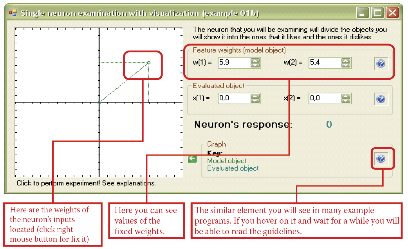
Example 01b is easy to operate. You simply need to click in the area on the left chart. First, click with the right button to set the location of chosen point corresponding to the neuron’s weight factors (see Figure 4.10). You will see the point and its coordinates. Of course, you can change values at any time by clicking again in another part of the chart or modifying the coordinates as we did in the Example 01a program.

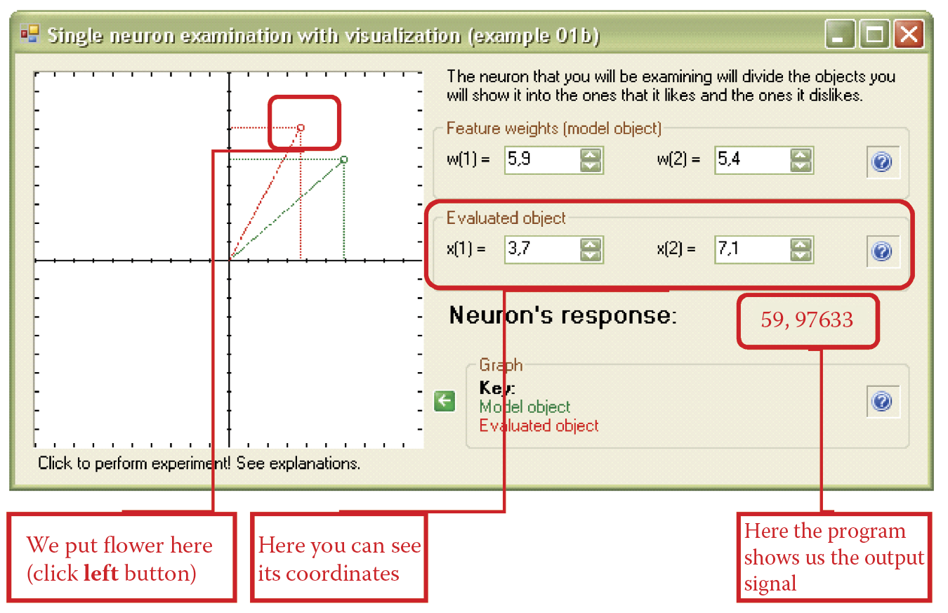
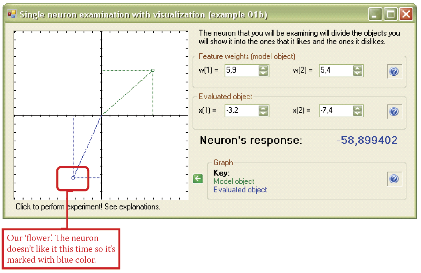
Now click on the chart with the left button to locate the position of the flower and watch the answer appear. If the neuron likes the flower (you can see what the neuron thinks of the flower from the value of the output signal on the right), the appropriate point is marked on the chart with red box (like a mountains on a map; see Figure 4.11). If the judgment is negative, the point is marked with blue box (like a seabed on a map; see Figure 4.12). When the reaction of the neuron is neutral, the corresponding point is light blue (Figure 4.13). You will soon be able to imagine how the areas corresponding to the decisions in the input space will appear. Also, you can drag the mouse pointer over the chart with one of the buttons pressed to see the results change.

4.4 Managing More Inputs

The examples above are clear and simple because they concern a single neuron with only two inputs. Real applications of neural networks typically involve tasks requiring many inputs. Problems solved by neural networks often depend on huge numbers of input data and many cooperating neurons must work cooperatively to generate an appropriate solution to a problem.

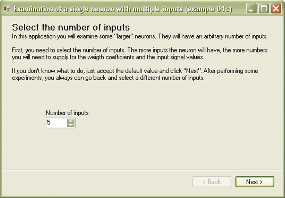
This point is difficult to illustrate. It would involve an input space of 10 or more dimensions! We suggest an alternative: the Example 01c program (Figure 4.14). The system asks the user to enter the number of neuron inputs. You can accept the default value (5) and click Next. As in Examples 01a and b, you then input the weights that define the model of the signal to which your neuron should react positively. Fill in the w(i) column shown in Figure 4.15, then enter the values of the input signals in the x(i) column. The program will then calculate the output. Simple, isn’t it?

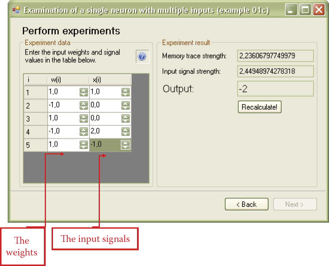
During experiments you will notice that high values of the output signals are returned in two situations: (1) when input signals correspond to the weights of the neuron as expected or (2) by entering huge input values where weights are positive. The first way of obtaining high output is intelligent, sophisticated, and elegant. The same (sometimes even better) effects can be obtained by using brute force and the second method.

When entering input signals, you should try to make them of the same strength using the parameter estimate given by the computer. This will enable you to correctly interpret and compare your results. Similarly, when comparing the behaviors of two neurons with different weight values to find identical input signals (they should have the same value of memory trace strength), the difference is the length of the weight vector. In a network with a great number of neurons, the meaning of the strength of the input signals radically decreases when stronger (better tuned) or weaker (worse tuned) input signals reach every neuron.

When we consider only one neuron, dissimilar values of input signals make results harder to interpret. That is why we should agree on choosing input values so that the sum of their squares is between 5 and 35, for example. The range is an estimate; great precision is not needed here. Because the program calculates the strength as a square root from the sum of squares of the coordinates (the formula for the length of a vector), the strength of the signals should be between the square root of 5 and the square root of 35—roughly between 2 and 6.

Why should we choose these values? While we were designing the program, we observed that entering small random integer values for five inputs of the neuron yielded more or less accurate values. If you prefer, you can choose any other value and it will work. The same suggestion for choosing values is useful for applying weights. Results are easier to check if the input signals “match” the values.

4.5 Network Functioning

Consider a network consisting of multiple neurons organized in a single layer. They are not connected to each other and each neuron handles input and output; see Figure 4.16. The input signals you apply will enter every neuron. The output signals of the neurons will be treated as the entire network’s response to a given task. How does this work?

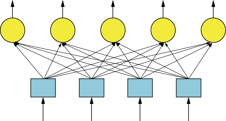
Every neuron has its own set of weights that make it ready to recognize certain characteristics of the input signals. Every neuron has different weights and recognizes different patterns of signals. When input signals are entered, every neuron will calculate its output signal independently. Some will generate high outputs because they recognize patterns and others will produce small outputs based on less recognition.

By analyzing the output signals, you can identify patterns the network “suggests” based on your observations of high output values. You can also evaluate how sure the network is of its decision by comparing the output signal of the “winning” neuron with the signals generated by other neurons.

Sometimes the ability of a network to detect uncertain situations is useful for limited types of problems. An algorithm that makes decisions based on incomplete data must be used wisely.

4.6 Construction of Simple Linear Neural Network

The network described in the Example 02 program recognizes three categories of animals (mammals, fish, and birds). This simple program will help you start a simple exercise with a very small neural network. We encourage you though to write a more complicated program to solve a simple but real problem.

The example network contains only three neurons. Recognitions are made based on five features (inputs). The following information about animal characteristics is input:

How many legs does it have?

Does it live in water or does it fly?

Is it covered with feathers?

Does it hatch from an egg?

For every neuron, the values of weights are set to match the pattern of a specific animal. Neuron 1 should recognize a mammal and utilizes the following weight values set:

Weight Value	Characteristic
4	Mammal has four legs
0.01	Mammal sometimes lives in water (e.g., seal); water is not typical milieu
0.01	Mammal sometimes flies (e.g., bat); flying is not typical activity
–1	Mammal has no feathers
1.5	Mammal is viviparous (major characteristic)

The weights of Neuron 2 are set to recognize birds using the same technique and different values:

Weight Value	Characteristic
2	Bird has two legs
–1	Bird does not live in water
2	Bird usually flies; ostriches are exceptions
2.5	Bird has feathers (major characteristic)
2	Bird hatches from egg

The weights of Neuron 3 for identifying fish are set in the following way:

Weight Value	Characteristic
–1	Fish has no legs
3.5	Fish lives in water
0.01	Fish cannot fly; flying fish are exceptions
–2	Fish is not covered with feathers or similar structures
1.5	Fish generally hatches from egg; viviparous fish are exceptions

After the program starts, it displays information on a screen about weights for every input of every neuron (Figure 4.17) and allows us to perform interesting experiments as described in the next section.

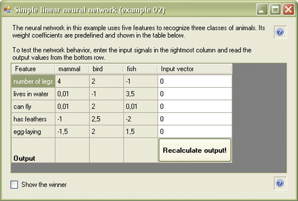
4.7 Use of Network

The program presented previously assumes that a network has three outputs associated with the recognition of three kinds of objects (animals): mammals, birds, and fish. The network has a single layer that contains only these three neurons. Later we will cover networks containing more neurons than the number of outputs. The simple construction of a neural network allows it to accommodate any number of outputs.

Our example involved the input of only five signals corresponding to certain features for recognizing objects. Obviously you can increase this number if your problem involves greater numbers of input data. All input signals are connected to every neuron according to the “lazy rule” that states: if you don’t feel like analyzing which input signal influences which output signal, the best choice is to connect everything to everything else. This concept has become common practice.

Despite the “lazy rule,” it is useful to think about input signals before entering them. Some contain numeric information (e.g., how many legs an animal has); others involve Boolean information (whether an animal lives in water, flies, is covered with feathers, or is viviparous). You should consider how you will represent logical values in a network because neurons operate, as we know, on the values of signals and not on symbols like true or false.

If you are a computer scientist, you may suspect that the idea of true and false can be expressed in binary form: 1 = true, 0 = false. If you are a great computer scientist who uses Assembler and dreams about microprocessor registry, hexadecimal memory records, and Java applets, this type of relation is obvious, total, and correct. We must confess that work in the area of neural networks will make you modify your habits as described below.

Remember that zero in a neural network is a useless signal to transfer because it carries no new information. Neurons work by multiplying signals by weights and then summing the result. Multiplying anything by zero always produces the same result regardless of the inner knowledge (value) of a neuron. By using zero as an input signal, you forego opportunities to learn and influence network behavior. That is why our program uses the convention of +1 = true and –1 = false. Such bipolar signals fulfill their tasks very well.

Another advantage of a bipolar neural network is the ability to use any values of input signals that may reflect the convictions of the user about the importance of certain information. When inserting data for a codfish, a crucial fact is that the fish lives in water so you may input +2 instead of +1. For other situations, you can input values smaller than one. You may have doubts about entering +1 in response to whether flying fish can fly if you entered +1 for an eagle that is a superb flier. In that case you can input +0.2 for the flying fish to indicate the uncertainty. Another example is the answer to a “has tail” signal for a snake. Based on snake anatomy, the answer may be +10.

Because we know how to handle network input signals, we can try a few simple experiments by inputting data for a few randomly chosen animals to check whether the network recognizes them correctly. In a network consisting of many elements, the normalization of input signals (considering signal strength) is not as crucial. The same result will be produced by the neuron if you describe an animal (e.g., fox), in this way:

Weight Value	Characteristic
4	Number of legs
–1	Does not live in water
–1	Does not fly
–0.9	Is not covered with feathers
–1	Viviparous

And the same result will be produced by the neuron if you describe such an animal like this:

Weight Value	Characteristic
8	Has 4 legs; legs are vital and thus counted twice
–6	Hates water
–3	Never flies
–5	Has no feathers; has fur (major characteristic)
–9	Does not lay eggs; is viviparous (major characteristic)

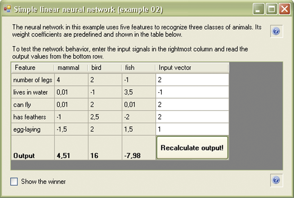
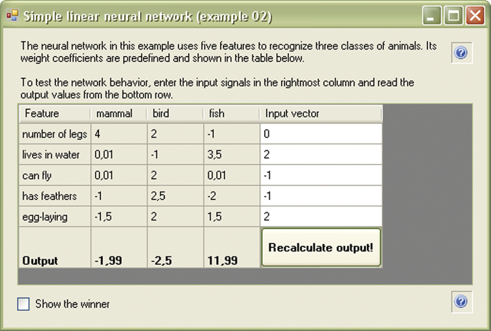
This simple network can recognize typical situations correctly. It will classify mammals, fish, and birds (Figure 4.18, Figure 4.19, and Figure 4.20) and also works well in atypical situations. For example, it will recognize a seal, bat, and even a platypus (a strange animal from Australia that hatches from an egg) as mammals. The network can also identify a non-flying ostrich as a bird and classify a flying fish correctly. Try it!

However, the network will be puzzled by a snake because the snake has no legs, lives on the ground, and hatches from eggs. When faced with a snake, every neuron in the network will decide the snake is not a decent animal and will thus generate a negative output. In the context of our classification, the output makes sense.

The three-neuron network is very primitive and sometimes makes mistakes. For example, it repeatedly recognizes turtle as a mammal (it has 4 legs, lives on land, but hatches from eggs) and classifies lungfish as mammals (they live on land during droughts). This demonstrates the need for a designer to set weights carefully and completely and monitor outputs consistently.

4.8 Rivalry in Neural Networks

In practical applications, a network sometimes requires an additional mechanism known as rivalry between neurons to improve its performance. In essence, the technique involves a competition that produces a winner. In our animal recognition example, an element would compare all the output signals select a winner—the neuron with a highest value of output signal. Selecting a winner may have consequences (as we will see in the discussion of Kohonen networks in Chapter 10). In most cases, the output signals of a network are polarized. Only the winner neuron can output its signal; every other output is zeroed. This is known as the winner-takes-all (WTA) rule. It simplifies the examination of networks that involve many outputs but presents a few disadvantages as noted.

We can introduce the element of rivalry into our Example 02 program simulating the recognition of animals. At the start of the program, select Show the winner. After processing the input data, the program will mark in red the neuron producing the highest output value (the winner). Examples appear in Figure 4.21 and Figure 4.22.

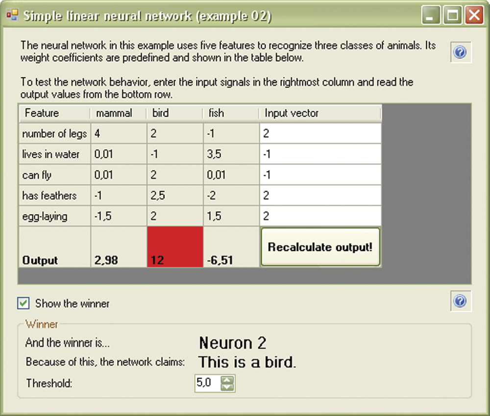
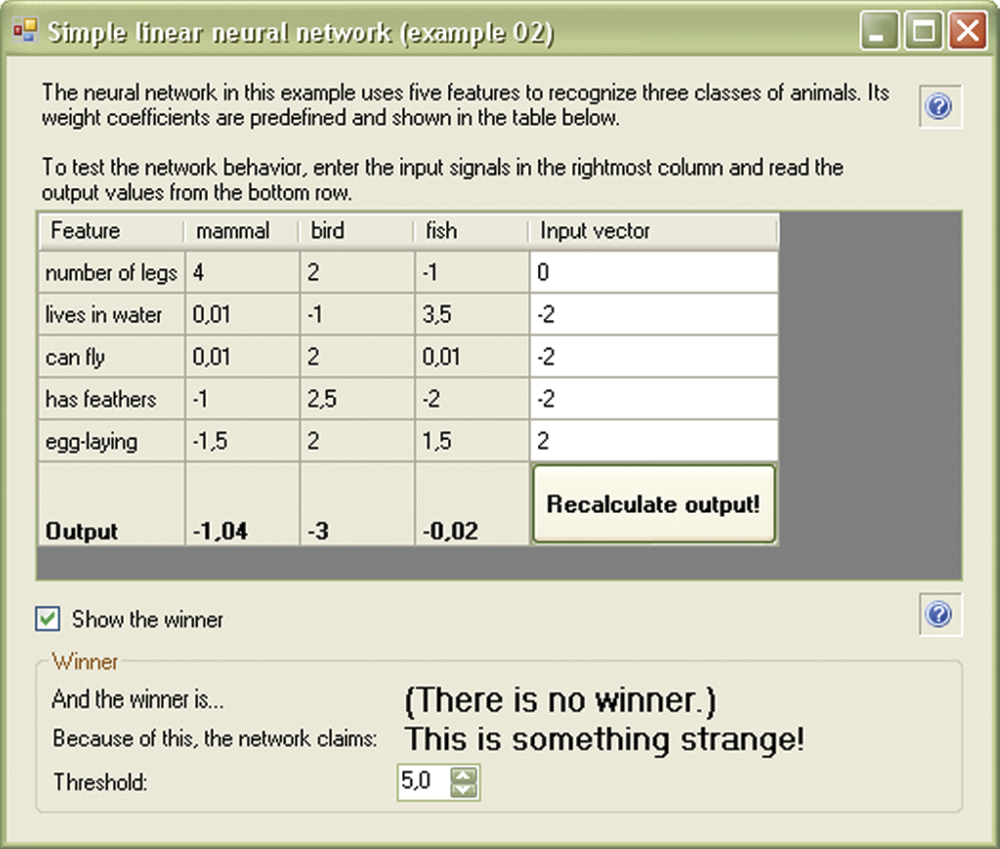
Note that we assume that only the positive value is a basis for a decision during a neuron competition. If every output signal is smaller than the value marked in the program as a threshold (set as you wish), the output signal should be a no-recognition signal.

We suggest you use program Example 02 to perform experiments involving rivalry of neurons. Despite the simplicity of a linear network, it functions effectively and provides answers as text instead of numbers that require further interpretation. These networks have limits as well that will be covered in subsequent chapters.

4.9 Additional Applications

The purpose of the network described in this chapter was to recognize some sets of information treated as a set of features of recognized objects. However, it is not the only application for a simple single-layered network consisting of neurons with linear characteristics. Networks of this type are often used for purposes such as signal filtering (especially as adaptive filters with properties that change according to current needs).

These networks also have numerous applications in signal transformation (speech, music, video, and medical diagnosis such as electrocardiogram, electroencephalogram, and electromyelogram instruments). Such networks can extract a spectrum of a signal or arrange input data using the principal components analysis method. These are only a few of many examples. Even a simple one-layer network can handle many types of applications.

All decisions of a network are made by a set of weights for every neuron. By setting the weights differently, we change the way a network works. In the same way, changing a program makes a computer work differently. In the examples described previously, we used a set of weights chosen arbitrarily. We had to determine a weight value for every neuron. This, of course, may be interpreted as a change of a work program for a network.

For a network containing few neurons that allows simple and obvious interpretation of the weight factors (as in our example of animal recognition), this “manual” programming can produce good results. However, in practical applications, networks contain many elements. It is thus impossible to determine the parameters of a single neuron and follow its operation. That is why more useful and flexible networks choose their own weights in the process of learning. Chapter 5 is dedicated to a vital aspect of neural network design: teaching.

Questions and Self-Study Tasks

1. Which of the following properties do a neuron’s weights and the input signals need to generate an output signal? Strong and positive? Strong and negative? Close to zero?

2. How can you make a neuron to favor one of its inputs (e.g., make the color of a flower more important than its fragrance)?

3. How can you interpret the positive and the negative values assigned to every input of a neuron?

4. How can you interpret the positive and the negative output signals of a neuron?

5. Does a neuron having all negative input values always generate a negative output signal?

6. Is there any limit to the number of neuron input signals?

7. Does the network modeled in the Example 02 program recognize a dolphin as a mammal or a fish?

8. What can be achieved by rivalry of neural network?

9. What animal group will a bat be assigned to by the network modeled in the Example 02 program?

10. Does the network modeled in the Example 02 program recognize that dinosaurs were not mammals, birds, or fish? They were reptiles but the example has no reptile category. Which animals known to the network do dinosaurs most closely resemble?

11. Does a network competition always have a winner? Is the answer good or bad?

12. Advanced exercise: In a neural network recognizing animals, add additional classes such as predators or herbivores and extra data describing features (sharpness of teeth or bills, speed, etc.).

---