
Chapter 3. Dictionaries and Sets
Any running Python program has many dictionaries active at the same time, even if the user’s program code doesn’t explicitly use a dictionary.
A. M. Kuchling, “Python’s Dictionary Implementation: Being All Things to All People”1
The dict type is not only widely used in our programs but also a fundamental part of the Python implementation. Module namespaces, class and instance attributes, and function keyword arguments are some of the fundamental constructs where dictionaries are deployed. The built-in functions live in __builtins__.__dict__.
Because of their crucial role, Python dicts are highly optimized. Hash tables are the engines behind Python’s high-performance dicts.
We also cover sets in this chapter because they are implemented with hash tables as well. Knowing how a hash table works is key to making the most of dictionaries and sets.
Here is a brief outline of this chapter:
-
Common dictionary methods
-
Special handling for missing keys
-
Variations of
dictin the standard library -
The
setandfrozensettypes -
How hash tables work
-
Implications of hash tables (key type limitations, unpredictable ordering, etc.)
Generic Mapping Types
The collections.abc module provides the Mapping and MutableMapping ABCs to formalize the interfaces of dict and similar types (in Python 2.6 to 3.2, these classes are imported from the collections module, and not from collections.abc). See Figure 3-1.
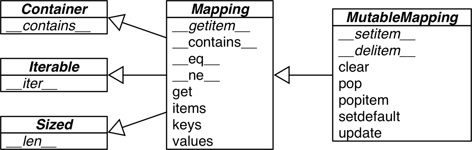
Figure 3-1. UML class diagram for the MutableMapping and its superclasses from collections.abc (inheritance arrows point from subclasses to superclasses; names in italic are abstract classes and abstract methods)
Implementations of specialized mappings often extend dict or collections.UserDict, instead of these ABCs. The main value of the ABCs is documenting and formalizing the minimal interfaces for mappings, and serving as criteria for isinstance tests in code that needs to support mappings in a broad sense:
>>>my_dict={}>>>isinstance(my_dict,abc.Mapping)True
Using isinstance is better than checking whether a function argument is of dict type, because then alternative mapping types can be used.
All mapping types in the standard library use the basic dict in their implementation, so they share the limitation that the keys must be hashable (the values need not be hashable, only the keys).
Given these ground rules, you can build dictionaries in several ways. The Built-in Types page in the Library Reference has this example to show the various means of building a dict:
>>>a=dict(one=1,two=2,three=3)>>>b={'one':1,'two':2,'three':3}>>>c=dict(zip(['one','two','three'],[1,2,3]))>>>d=dict([('two',2),('one',1),('three',3)])>>>e=dict({'three':3,'one':1,'two':2})>>>a==b==c==d==eTrue
In addition to the literal syntax and the flexible dict constructor, we can use dict comprehensions to build dictionaries. See the next section.
dict Comprehensions
Since Python 2.7, the syntax of listcomps and genexps was applied to dict comprehensions (and set comprehensions as well, which we’ll soon visit). A dictcomp builds a dict instance by producing key:value pair from any iterable. Example 3-1 shows the use of dict comprehensions to build two dictionaries from the same list of tuples.
Example 3-1. Examples of dict comprehensions
>>>DIAL_CODES=[...(86,'China'),...(91,'India'),...(1,'United States'),...(62,'Indonesia'),...(55,'Brazil'),...(92,'Pakistan'),...(880,'Bangladesh'),...(234,'Nigeria'),...(7,'Russia'),...(81,'Japan'),...]>>>country_code={country:codeforcode,countryinDIAL_CODES}>>>country_code{'China': 86, 'India': 91, 'Bangladesh': 880, 'United States': 1,'Pakistan': 92, 'Japan': 81, 'Russia': 7, 'Brazil': 55, 'Nigeria':234, 'Indonesia': 62}>>>{code:country.upper()forcountry,codeincountry_code.items()...ifcode<66}{1: 'UNITED STATES', 55: 'BRAZIL', 62: 'INDONESIA', 7: 'RUSSIA'}

A list of pairs can be used directly with the
dictconstructor.
Here the pairs are reversed:
countryis the key, andcodeis the value.
Reversing the pairs again, values uppercased and items filtered by
code < 66.
If you’re used to liscomps, dictcomps are a natural next step. If you aren’t, the spread of the listcomp syntax means it’s now more profitable than ever to become fluent in it.
We now move to a panoramic view of the API for mappings.
Overview of Common Mapping Methods
The basic API for mappings is quite rich. Table 3-1 shows the methods implemented by dict and two of its most useful variations: defaultdict and OrderedDict, both defined in the collections module.
| dict | defaultdict | OrderedDict | ||
|---|---|---|---|---|
|
● |
● |
● |
Remove all items |
|
● |
● |
● |
|
|
● |
● |
● |
Shallow copy |
|
● |
Support for |
||
|
● |
Callable invoked by |
||
|
● |
● |
● |
|
|
● |
● |
● |
New mapping from keys in iterable, with optional initial value (defaults to |
|
● |
● |
● |
Get item with key |
|
● |
● |
● |
|
|
● |
● |
● |
Get view over items— |
|
● |
● |
● |
Get iterator over keys |
|
● |
● |
● |
Get view over keys |
|
● |
● |
● |
|
|
● |
Called when |
||
|
● |
Move |
||
|
● |
● |
● |
Remove and return value at |
|
● |
● |
● |
Remove and return an arbitrary |
|
● |
Get iterator for keys from last to first inserted |
||
|
● |
● |
● |
If |
|
● |
● |
● |
|
|
● |
● |
● |
Update |
|
● |
● |
● |
Get view over values |
a b | ||||
The way update handles its first argument m is a prime example of duck typing: it first checks whether m has a keys method and, if it does, assumes it is a mapping. Otherwise, update falls back to iterating over m, assuming its items are (key, value) pairs. The constructor for most Python mappings uses the logic of update internally, which means they can be initialized from other mappings or from any iterable object producing (key, value) pairs.
A subtle mapping method is setdefault. We don’t always need it, but when we do, it provides a significant speedup by avoiding redundant key lookups. If you are not comfortable using it, the following section explains how, through a practical example.
Handling Missing Keys with setdefault
In line with the fail-fast philosophy, dict access with d[k] raises an error when k is not an existing key. Every Pythonista knows that d.get(k, default) is an alternative to d[k] whenever a default value is more convenient than handling KeyError. However, when updating the value found (if it is mutable), using either __getitem__ or get is awkward and inefficient. Consider Example 3-2, a suboptimal script written just to show one case where dict.get is not the best way to handle a missing key.
Example 3-2 is adapted from an example by Alex Martelli,2 which generates an index like that in Example 3-3.
Example 3-2. index0.py uses dict.get to fetch and update a list of word occurrences from the index (a better solution is in Example 3-4)
"""Build an index mapping word -> list of occurrences"""importsysimportreWORD_RE=re.compile(r'w+')index={}withopen(sys.argv[1],encoding='utf-8')asfp:forline_no,lineinenumerate(fp,1):formatchinWORD_RE.finditer(line):word=match.group()column_no=match.start()+1location=(line_no,column_no)# this is ugly; coded like this to make a pointoccurrences=index.get(word,[])occurrences.append(location)index[word]=occurrences# print in alphabetical orderforwordinsorted(index,key=str.upper):(word,index[word])
Get the list of occurrences for
word, or[]if not found.Append new location to
occurrences.Put changed
occurrencesintoindexdict; this entails a second search through theindex.
In the
key=argument ofsortedI am not callingstr.upper, just passing a reference to that method so thesortedfunction can use it to normalize the words for sorting.3
Example 3-3. Partial output from Example 3-2 processing the Zen of Python; each line shows a word and a list of occurrences coded as pairs: (line-number, column-number)
$python3 index0.py ../../data/zen.txt a[(19, 48),(20, 53)]Although[(11, 1),(16, 1),(18, 1)]ambiguity[(14, 16)]and[(15, 23)]are[(21, 12)]aren[(10, 15)]at[(16, 38)]bad[(19, 50)]be[(15, 14),(16, 27),(20, 50)]beats[(11, 23)]Beautiful[(3, 1)]better[(3, 14),(4, 13),(5, 11),(6, 12),(7, 9),(8, 11),(17, 8),(18, 25)]...
The three lines dealing with occurrences in Example 3-2 can be replaced by a single line using dict.setdefault. Example 3-4 is closer to Alex Martelli’s original example.
Example 3-4. index.py uses dict.setdefault to fetch and update a list of word occurrences from the index in a single line; contrast with Example 3-2
"""Build an index mapping word -> list of occurrences"""importsysimportreWORD_RE=re.compile(r'w+')index={}withopen(sys.argv[1],encoding='utf-8')asfp:forline_no,lineinenumerate(fp,1):formatchinWORD_RE.finditer(line):word=match.group()column_no=match.start()+1location=(line_no,column_no)index.setdefault(word,[]).append(location)# print in alphabetical orderforwordinsorted(index,key=str.upper):(word,index[word])
Get the list of occurrences for
word, or set it to[]if not found;setdefaultreturns the value, so it can be updated without requiring a second search.
In other words, the end result of this line…
my_dict.setdefault(key,[]).append(new_value)
…is the same as running…
ifkeynotinmy_dict:my_dict[key]=[]my_dict[key].append(new_value)
…except that the latter code performs at least two searches for key—three if it’s not found—while setdefault does it all with a single lookup.
A related issue, handling missing keys on any lookup (and not only when inserting), is the subject of the next section.
Mappings with Flexible Key Lookup
Sometimes it is convenient to have mappings that return some made-up value when a missing key is searched. There are two main approaches to this: one is to use a defaultdict instead of a plain dict. The other is to subclass dict or any other mapping type and add a __missing__ method. Both solutions are covered next.
defaultdict: Another Take on Missing Keys
Example 3-5 uses collections.defaultdict to provide another elegant solution to the problem in Example 3-4. A defaultdict is configured to create items on demand whenever a missing key is searched.
Here is how it works: when instantiating a defaultdict, you provide a callable that is used to produce a default value whenever __getitem__ is passed a nonexistent key argument.
For example, given an empty defaultdict created as dd = defaultdict(list), if 'new-key' is not in dd, the expression dd['new-key'] does the following steps:
-
Calls
list()to create a new list. -
Inserts the list into
ddusing'new-key'as key. -
Returns a reference to that list.
The callable that produces the default values is held in an instance attribute called default_factory.
Example 3-5. index_default.py: using an instance of defaultdict instead of the setdefault method
"""Build an index mapping word -> list of occurrences"""importsysimportreimportcollectionsWORD_RE=re.compile(r'w+')index=collections.defaultdict(list)withopen(sys.argv[1],encoding='utf-8')asfp:forline_no,lineinenumerate(fp,1):formatchinWORD_RE.finditer(line):word=match.group()column_no=match.start()+1location=(line_no,column_no)index[word].append(location)# print in alphabetical orderforwordinsorted(index,key=str.upper):(word,index[word])
Create a
defaultdictwith thelistconstructor asdefault_factory.If
wordis not initially in theindex, thedefault_factoryis called to produce the missing value, which in this case is an emptylistthat is then assigned toindex[word]and returned, so the.append(location)operation always succeeds.
If no default_factory is provided, the usual KeyError is raised for missing keys.
Warning
The default_factory of a defaultdict is only invoked to provide default values for __getitem__ calls, and not for the other methods. For example, if dd is a defaultdict, and k is a missing key, dd[k] will call the default_factory to create a default value, but dd.get(k) still returns None.
The mechanism that makes defaultdict work by calling default_factory is actually the __missing__ special method, a feature supported by all standard mapping types that we discuss next.
The __missing__ Method
Underlying the way mappings deal with missing keys is the aptly named __missing__ method. This method is not defined in the base dict class, but dict is aware of it: if you subclass dict and provide a __missing__ method, the standard dict.__getitem__ will call it whenever a key is not found, instead of raising KeyError.
Warning
The __missing__ method is just called by __getitem__ (i.e., for the d[k] operator). The presence of a __missing__ method has no effect on the behavior of other methods that look up keys, such as get or __contains__ (which implements the in operator). This is why the default_factory of defaultdict works only with __getitem__, as noted in the warning at the end of the previous section.
Suppose you’d like a mapping where keys are converted to str when looked up. A concrete use case is the Pingo.io project, where a programmable board with GPIO pins (e.g., the Raspberry Pi or the Arduino) is represented by a board object with a board.pins attribute, which is a mapping of physical pin locations to pin objects, and the physical location may be just a number or a string like "A0" or "P9_12". For consistency, it is desirable that all keys in board.pins are strings, but it is also convenient that looking up my_arduino.pin[13] works as well, so beginners are not tripped when they want to blink the LED on pin 13 of their Arduinos. Example 3-6 shows how such a mapping would work.
Example 3-6. When searching for a nonstring key, StrKeyDict0 converts it to str when it is not found
Testsforitemretrievalusing`d[key]`notation::>>>d=StrKeyDict0([('2','two'),('4','four')])>>>d['2']'two'>>>d[4]'four'>>>d[1]Traceback(mostrecentcalllast):...KeyError:'1'Testsforitemretrievalusing`d.get(key)`notation::>>>d.get('2')'two'>>>d.get(4)'four'>>>d.get(1,'N/A')'N/A'Testsforthe`in`operator::>>>2indTrue>>>1indFalse
Example 3-7 implements a class StrKeyDict0 that passes the preceding tests.
Note
A better way to create a user-defined mapping type is to subclass collections.UserDict instead of dict (as we’ll do in Example 3-8). Here we subclass dict just to show that __missing__ is supported by the built-in dict.__getitem__ method.
Example 3-7. StrKeyDict0 converts nonstring keys to str on lookup (see tests in Example 3-6)
classStrKeyDict0(dict):def__missing__(self,key):ifisinstance(key,str):raiseKeyError(key)returnself[str(key)]defget(self,key,default=None):try:returnself[key]exceptKeyError:returndefaultdef__contains__(self,key):returnkeyinself.keys()orstr(key)inself.keys()
StrKeyDict0inherits fromdict.Check whether
keyis already astr. If it is, and it’s missing, raiseKeyError.Build
strfromkeyand look it up.The
getmethod delegates to__getitem__by using theself[key]notation; that gives the opportunity for our__missing__to act.
If a
KeyErrorwas raised,__missing__already failed, so we return thedefault.
Search for unmodified key (the instance may contain non-
strkeys), then for astrbuilt from the key.
Take a moment to consider why the test isinstance(key, str) is necessary in the __missing__ implementation.
Without that test, our __missing__ method would work OK for any key k—str or not str—whenever str(k) produced an existing key. But if str(k) is not an existing key, we’d have an infinite recursion. The last line, self[str(key)] would call __getitem__ passing that str key, which in turn would call __missing__ again.
The __contains__ method is also needed for consistent behavior in this example, because the operation k in d calls it, but the method inherited from dict does not fall back to invoking __missing__. There is a subtle detail in our implementation of __contains__: we do not check for the key in the usual Pythonic way—k in my_dict—because str(key) in self would recursively call __contains__. We avoid this by explicitly looking up the key in self.keys().
Note
A search like k in my_dict.keys() is efficient in Python 3 even for very large mappings because dict.keys() returns a view, which is similar to a set, and containment checks in sets are as fast as in dictionaries. Details are documented in the “Dictionary” view objects section of the documentation. In Python 2, dict.keys() returns a list, so our solution also works there, but it is not efficient for large dictionaries, because k in my_list must scan the list.
The check for the unmodified key—key in self.keys()—is necessary for correctness because StrKeyDict0 does not enforce that all keys in the dictionary must be of type str. Our only goal with this simple example is to make searching “friendlier” and not enforce types.
So far we have covered the dict and defaultdict mapping types, but the standard library comes with other mapping implementations, which we discuss next.
Variations of dict
In this section, we summarize the various mapping types included in the collections module of the standard library, besides defaultdict:
collections.OrderedDict-
Maintains keys in insertion order, allowing iteration over items in a predictable order. The
popitemmethod of anOrderedDictpops the last item by default, but if called asmy_odict.popitem(last=False), it pops the first item added. collections.ChainMap-
Holds a list of mappings that can be searched as one. The lookup is performed on each mapping in order, and succeeds if the key is found in any of them. This is useful to interpreters for languages with nested scopes, where each mapping represents a scope context. The “ChainMap objects” section of the
collectionsdocs has several examples ofChainMapusage, including this snippet inspired by the basic rules of variable lookup in Python:importbuiltinspylookup=ChainMap(locals(),globals(),vars(builtins)) collections.Counter-
A mapping that holds an integer count for each key. Updating an existing key adds to its count. This can be used to count instances of hashable objects (the keys) or as a multiset—a set that can hold several occurrences of each element.
Counterimplements the+and-operators to combine tallies, and other useful methods such asmost_common([n]), which returns an ordered list of tuples with the n most common items and their counts; see the documentation. Here isCounterused to count letters in words:>>>ct=collections.Counter('abracadabra')>>>ctCounter({'a': 5, 'b': 2, 'r': 2, 'c': 1, 'd': 1})>>>ct.update('aaaaazzz')>>>ctCounter({'a': 10, 'z': 3, 'b': 2, 'r': 2, 'c': 1, 'd': 1})>>>ct.most_common(2)[('a', 10), ('z', 3)] collections.UserDict-
A pure Python implementation of a mapping that works like a standard
dict.
While OrderedDict, ChainMap, and Counter come ready to use, UserDict is designed to be subclassed, as we’ll do next.
Subclassing UserDict
It’s almost always easier to create a new mapping type by extending UserDict rather than dict. Its value can be appreciated as we extend our StrKeyDict0 from Example 3-7 to make sure that any keys added to the mapping are stored as str.
The main reason why it’s preferable to subclass from UserDict rather than from dict is that the built-in has some implementation shortcuts that end up forcing us to override methods that we can just inherit from UserDict with no problems.4
Note that UserDict does not inherit from dict, but has an internal dict instance, called data, which holds the actual items. This avoids undesired recursion when coding special methods like __setitem__, and simplifies the coding of __contains__, compared to Example 3-7.
Thanks to UserDict, StrKeyDict (Example 3-8) is actually shorter than StrKeyDict0 (Example 3-7), but it does more: it stores all keys as str, avoiding unpleasant surprises if the instance is built or updated with data containing nonstring keys.
Example 3-8. StrKeyDict always converts non-string keys to str—on insertion, update, and lookup
importcollectionsclassStrKeyDict(collections.UserDict):def__missing__(self,key):ifisinstance(key,str):raiseKeyError(key)returnself[str(key)]def__contains__(self,key):returnstr(key)inself.datadef__setitem__(self,key,item):self.data[str(key)]=item
StrKeyDictextendsUserDict.__missing__is exactly as in Example 3-7.__contains__is simpler: we can assume all stored keys arestrand we can check onself.datainstead of invokingself.keys()as we did inStrKeyDict0.__setitem__converts anykeyto astr. This method is easier to overwrite when we can delegate to theself.dataattribute.
Because UserDict subclasses MutableMapping, the remaining methods that make StrKeyDict a full-fledged mapping are inherited from UserDict, MutableMapping, or Mapping. The latter have several useful concrete methods, in spite of being abstract base classes (ABCs). The following methods are worth noting:
MutableMapping.update-
This powerful method can be called directly but is also used by
__init__to load the instance from other mappings, from iterables of(key, value)pairs, and keyword arguments. Because it usesself[key] = valueto add items, it ends up calling our implementation of__setitem__. Mapping.get-
In
StrKeyDict0(Example 3-7), we had to code our owngetto obtain results consistent with__getitem__, but in Example 3-8 we inheritedMapping.get, which is implemented exactly likeStrKeyDict0.get(see Python source code).
Tip
After I wrote StrKeyDict, I discovered that Antoine Pitrou authored PEP 455 — Adding a key-transforming dictionary to collections and a patch to enhance the collections module with a TransformDict. The patch is attached to issue18986 and may land in Python 3.5. To experiment with TransformDict, I extracted it into a standalone module (03-dict-set/transformdict.py in the Fluent Python code repository). TransformDict is more general than StrKeyDict, and is complicated by the requirement to preserve the keys as they were originally inserted.
We know there are several immutable sequence types, but how about an immutable dictionary? Well, there isn’t a real one in the standard library, but a stand-in is available. Read on.
Immutable Mappings
The mapping types provided by the standard library are all mutable, but you may need to guarantee that a user cannot change a mapping by mistake. A concrete use case can be found, again, in the Pingo.io project I described in “The __missing__ Method”: the board.pins mapping represents the physical GPIO pins on the device. As such, it’s nice to prevent inadvertent updates to board.pins because the hardware can’t possibly be changed via software, so any change in the mapping would make it inconsistent with the physical reality of the device.
Since Python 3.3, the types module provides a wrapper class called MappingProxyType, which, given a mapping, returns a mappingproxy instance that is a read-only but dynamic view of the original mapping. This means that updates to the original mapping can be seen in the mappingproxy, but changes cannot be made through it. See Example 3-9 for a brief demonstration.
Example 3-9. MappingProxyType builds a read-only mappingproxy instance from a dict
>>>fromtypesimportMappingProxyType>>>d={1:'A'}>>>d_proxy=MappingProxyType(d)>>>d_proxymappingproxy({1: 'A'})>>>d_proxy[1]'A'>>>d_proxy[2]='x'Traceback (most recent call last):File"<stdin>", line1, in<module>TypeError:'mappingproxy' object does not support item assignment>>>d[2]='B'>>>d_proxymappingproxy({1: 'A', 2: 'B'})>>>d_proxy[2]'B'>>>
Items in
dcan be seen throughd_proxy.Changes cannot be made through
d_proxy.d_proxyis dynamic: any change indis reflected.
Here is how this could be used in practice in the Pingo.io scenario: the constructor in a concrete Board subclass would fill a private mapping with the pin objects, and expose it to clients of the API via a public .pins attribute implemented as a mappingproxy. That way the clients would not be able to add, remove, or change pins by accident.5
Now that we’ve covered most mapping types in the standard library and when to use them, we will move to the set types.
Set Theory
Sets are a relatively new addition in the history of Python, and somewhat underused. The set type and its immutable sibling frozenset first appeared in a module in Python 2.3 and were promoted to built-ins in Python 2.6.
Note
In this book, the word “set” is used to refer both to set and frozenset. When talking specifically about the set class, its name appears in the constant width font used for source code: set.
A set is a collection of unique objects. A basic use case is removing duplication:
>>>l=['spam','spam','eggs','spam']>>>set(l){'eggs', 'spam'}>>>list(set(l))['eggs', 'spam']
Set elements must be hashable. The set type is not hashable, but frozenset is, so you can have frozenset elements inside a set.
In addition to guaranteeing uniqueness, the set types implement the essential set operations as infix operators, so, given two sets a and b, a | b returns their union, a & b computes the intersection, and a - b the difference. Smart use of set operations can reduce both the line count and the runtime of Python programs, at the same time making code easier to read and reason about—by removing loops and lots of conditional logic.
For example, imagine you have a large set of email addresses (the haystack) and a smaller set of addresses (the needles) and you need to count how many needles occur in the haystack. Thanks to set intersection (the & operator) you can code that in a simple line (see Example 3-10).
Example 3-10. Count occurrences of needles in a haystack, both of type set
found=len(needles&haystack)
Without the intersection operator, you’d have write Example 3-11 to accomplish the same task as Example 3-10.
Example 3-11. Count occurrences of needles in a haystack (same end result as Example 3-10)
found=0forninneedles:ifninhaystack:found+=1
Example 3-10 runs slightly faster than Example 3-11. On the other hand, Example 3-11 works for any iterable objects needles and haystack, while Example 3-10 requires that both be sets. But, if you don’t have sets on hand, you can always build them on the fly, as shown in Example 3-12.
Example 3-12. Count occurrences of needles in a haystack; these lines work for any iterable types
found=len(set(needles)&set(haystack))# another way:found=len(set(needles).intersection(haystack))
Of course, there is an extra cost involved in building the sets in Example 3-12, but if either the needles or the haystack is already a set, the alternatives in Example 3-12 may be cheaper than Example 3-11.
Any one of the preceding examples are capable of searching 1,000 values in a haystack of 10,000,000 items in a little over 3 milliseconds—that’s about 3 microseconds per needle.
Besides the extremely fast membership test (thanks to the underlying hash table), the set and frozenset built-in types provide a rich selection of operations to create new sets or, in the case of set, to change existing ones. We will discuss the operations shortly, but first a note about syntax.
set Literals
The syntax of set literals—{1}, {1, 2}, etc.—looks exactly like the math notation, with one important exception: there’s no literal notation for the empty set, so we must remember to write set().
Syntax Quirk
Don’t forget: to create an empty set, you should use the constructor without an argument: set(). If you write {}, you’re creating an empty dict—this hasn’t changed.
In Python 3, the standard string representation of sets always uses the {...} notation, except for the empty set:
>>>s={1}>>>type(s)<class 'set'>>>>s{1}>>>s.pop()1>>>sset()
Literal set syntax like {1, 2, 3} is both faster and more readable than calling the constructor (e.g., set([1, 2, 3])). The latter form is slower because, to evaluate it, Python has to look up the set name to fetch the constructor, then build a list, and finally pass it to the constructor. In contrast, to process a literal like {1, 2, 3}, Python runs a specialized BUILD_SET bytecode.
There is no special syntax to represent frozenset literals—they must be created by calling the constructor. The standard string representation in Python 3 looks like a frozenset constructor call. Note the output in the console session:
>>>frozenset(range(10))frozenset({0, 1, 2, 3, 4, 5, 6, 7, 8, 9})
Speaking of syntax, the familiar shape of listcomps was adapted to build sets as well.
Set Comprehensions
Set comprehensions (setcomps) were added in Python 2.7, together with the dictcomps that we saw in “dict Comprehensions”. Example 3-13 is a simple example.
Example 3-13. Build a set of Latin-1 characters that have the word “SIGN” in their Unicode names
>>>fromunicodedataimportname>>>{chr(i)foriinrange(32,256)if'SIGN'inname(chr(i),'')}{'§', '=', '¢', '#', '¤', '<', '¥', 'µ', '×', '$', '¶', '£', '©','°', '+', '÷', '±', '>', '¬', '®', '%'}
Import
namefunction fromunicodedatato obtain character names.Build set of characters with codes from 32 to 255 that have the word
'SIGN'in their names.
Syntax matters aside, let’s now review the rich assortment of operations provided by sets.
Set Operations
Figure 3-2 gives an overview of the methods you can expect from mutable and immutable sets. Many of them are special methods for operator overloading. Table 3-2 shows the math set operators that have corresponding operators or methods in Python. Note that some operators and methods perform in-place changes on the target set (e.g., &=, difference_update, etc.). Such operations make no sense in the ideal world of mathematical sets, and are not implemented in frozenset.
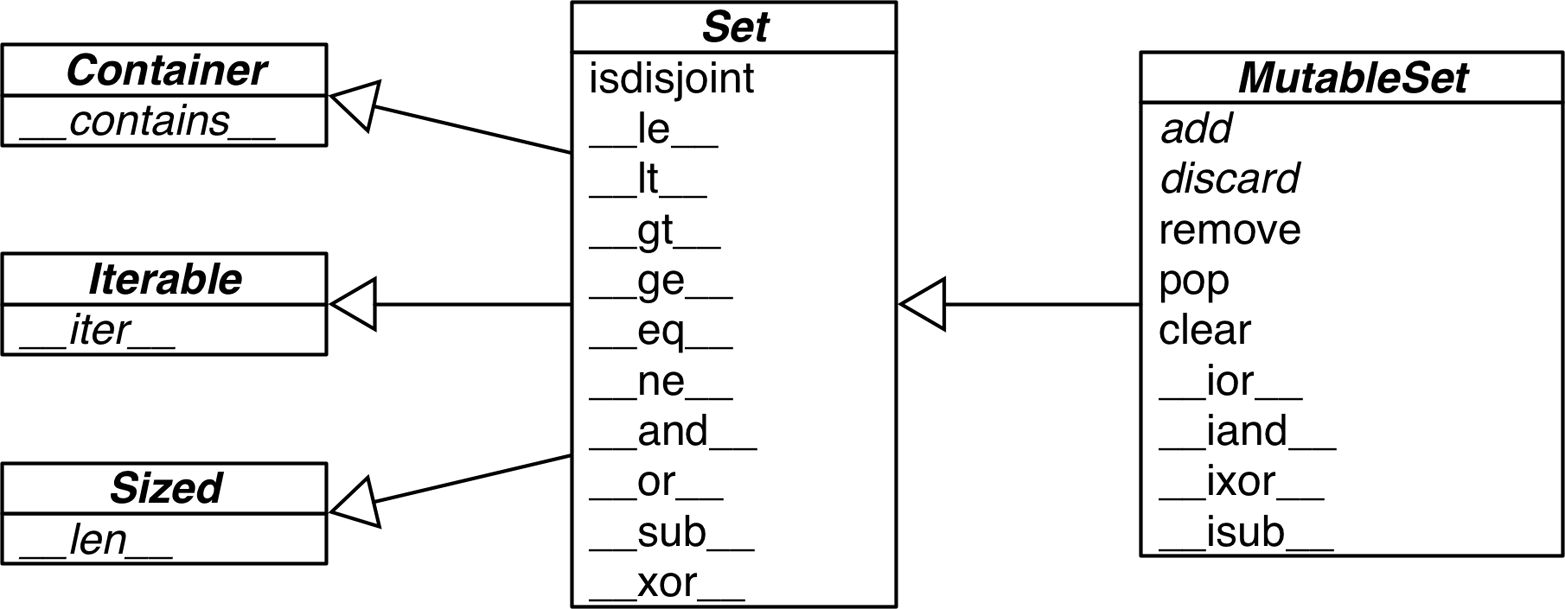
Figure 3-2. UML class diagram for MutableSet and its superclasses from collections.abc (names in italic are abstract classes and abstract methods; reverse operator methods omitted for brevity)
Tip
The infix operators in Table 3-2 require that both operands be sets, but all other methods take one or more iterable arguments. For example, to produce the union of four collections, a, b, c, and d, you can call a.union(b, c, d), where a must be a set, but b, c, and d can be iterables of any type.
| Math symbol | Python operator | Method | Description |
|---|---|---|---|
S ∩ Z |
|
|
Intersection of |
|
|
Reversed |
|
|
Intersection of |
||
|
|
|
|
|
|
||
S ∪ Z |
|
|
Union of |
|
|
Reversed |
|
|
Union of |
||
|
|
|
|
|
|
||
S Z |
|
|
Relative complement or difference between |
|
|
Reversed |
|
|
Difference between |
||
|
|
|
|
|
|
||
|
Complement of |
||
S ∆ Z |
|
|
Symmetric difference (the complement of the intersection |
|
|
Reversed |
|
|
|
||
|
|
|
Warning
As I write this, there is a Python bug report—(issue 8743)—that says: “The set() operators (or, and, sub, xor, and their in-place counterparts) require that the parameter also be an instance of set().”, with the undesired side effect that these operators don’t work with collections.abc.Set subclasses. The bug is already fixed in trunk for Python 2.7 and 3.4, and should be history by the time you read this.
Table 3-3 lists set predicates: operators and methods that return True or False.
| Math symbol | Python operator | Method | Description |
|---|---|---|---|
|
|
||
e ∈ S |
|
|
Element |
S ⊆ Z |
|
|
|
|
|
||
S ⊂ Z |
|
|
|
S ⊇ Z |
|
|
|
|
|
||
S ⊃ Z |
|
|
|
In addition to the operators and methods derived from math set theory, the set types implement other methods of practical use, summarized in Table 3-4.
| set | frozenset | ||
|---|---|---|---|
|
● |
Add element |
|
|
● |
Remove all elements of |
|
|
● |
● |
Shallow copy of |
|
● |
Remove element |
|
|
● |
● |
Get iterator over |
|
● |
● |
|
|
● |
Remove and return an element from |
|
|
● |
Remove element |
This completes our overview of the features of sets.
We now change gears to discuss how dictionaries and sets are implemented with hash tables. After reading the rest of this chapter, you will no longer be surprised by the apparently unpredictable behavior sometimes exhibited by dict, set, and their brethren.
dict and set Under the Hood
Understanding how Python dictionaries and sets are implemented using hash tables is helpful to make sense of their strengths and limitations.
Here are some questions this section will answer:
-
How efficient are Python
dictandset? -
Why are they unordered?
-
Why can’t we use any Python object as a
dictkey orsetelement? -
Why does the order of the
dictkeys orsetelements depend on insertion order, and may change during the lifetime of the structure? -
Why is it bad to add items to a
dictorsetwhile iterating through it?
To motivate the study of hash tables, we start by showcasing the amazing performance of dict and set with a simple test involving millions of items.
A Performance Experiment
From experience, all Pythonistas know that dicts and sets are fast. We’ll confirm that with a controlled experiment.
To see how the size of a dict, set, or list affects the performance of search using the in operator, I generated an array of 10 million distinct double-precision floats, the “haystack.” I then generated an array of needles: 1,000 floats, with 500 picked from the haystack and 500 verified not to be in it.
For the dict benchmark, I used dict.fromkeys() to create a dict named haystack with 1,000 floats. This was the setup for the dict test. The actual code I clocked with the timeit module is Example 3-14 (like Example 3-11).
Example 3-14. Search for needles in haystack and count those found
found=0forninneedles:ifninhaystack:found+=1
The benchmark was repeated another four times, each time increasing tenfold the size of haystack, to reach a size of 10,000,000 in the last test. The result of the dict performance test is in Table 3-5.
| len of haystack | Factor | dict time | Factor |
|---|---|---|---|
1,000 |
1x |
0.000202s |
1.00x |
10,000 |
10x |
0.000140s |
0.69x |
100,000 |
100x |
0.000228s |
1.13x |
1,000,000 |
1,000x |
0.000290s |
1.44x |
10,000,000 |
10,000x |
0.000337s |
1.67x |
In concrete terms, to check for the presence of 1,000 floating-point keys in a dictionary with 1,000 items, the processing time on my laptop was 0.000202s, and the same search in a dict with 10,000,000 items took 0.000337s. In other words, the time per search in the haystack with 10 million items was 0.337µs for each needle—yes, that is about one third of a microsecond per needle.
To compare, I repeated the benchmark, with the same haystacks of increasing size, but storing the haystack as a set or as list. For the set tests, in addition to timing the for loop in Example 3-14, I also timed the one-liner in Example 3-15, which produces the same result: count the number of elements from needles that are also in haystack.
Example 3-15. Use set intersection to count the needles that occur in haystack
found=len(needles&haystack)
Table 3-6 shows the tests side by side. The best times are in the “set& time” column, which displays results for the set & operator using the code from Example 3-15. The worst times are—as expected—in the “list time” column, because there is no hash table to support searches with the in operator on a list, so a full scan must be made, resulting in times that grow linearly with the size of the haystack.
| len of haystack | Factor | dict time | Factor | set time | Factor | set& time | Factor | list time | Factor |
|---|---|---|---|---|---|---|---|---|---|
1,000 |
1x |
0.000202s |
1.00x |
0.000143s |
1.00x |
0.000087s |
1.00x |
0.010556s |
1.00x |
10,000 |
10x |
0.000140s |
0.69x |
0.000147s |
1.03x |
0.000092s |
1.06x |
0.086586s |
8.20x |
100,000 |
100x |
0.000228s |
1.13x |
0.000241s |
1.69x |
0.000163s |
1.87x |
0.871560s |
82.57x |
1,000,000 |
1,000x |
0.000290s |
1.44x |
0.000332s |
2.32x |
0.000250s |
2.87x |
9.189616s |
870.56x |
10,000,000 |
10,000x |
0.000337s |
1.67x |
0.000387s |
2.71x |
0.000314s |
3.61x |
97.948056s |
9,278.90x |
If your program does any kind of I/O, the lookup time for keys in dicts or sets is negligible, regardless of the dict or set size (as long as it does fit in RAM). See the code used to generate Table 3-6 and accompanying discussion in Appendix A, Example A-1.
Now that we have concrete evidence of the speed of dicts and sets, let’s explore how that is achieved. The discussion of the hash table internals explains, for example, why the key ordering is apparently random and unstable.
Hash Tables in Dictionaries
This is a high-level view of how Python uses a hash table to implement a dict. Many details are omitted—the CPython code has some optimization tricks6—but the overall description is accurate.
Note
To simplify the ensuing presentation, we will focus on the internals of dict first, and later transfer the concepts to sets.
A hash table is a sparse array (i.e., an array that always has empty cells). In standard data structure texts, the cells in a hash table are often called “buckets.” In a dict hash table, there is a bucket for each item, and it contains two fields: a reference to the key and a reference to the value of the item. Because all buckets have the same size, access to an individual bucket is done by offset.
Python tries to keep at least 1/3 of the buckets empty; if the hash table becomes too crowded, it is copied to a new location with room for more buckets.
To put an item in a hash table, the first step is to calculate the hash value of the item key, which is done with the hash() built-in function, explained next.
Hashes and equality
The hash() built-in function works directly with built-in types and falls back to calling __hash__ for user-defined types. If two objects compare equal, their hash values must also be equal, otherwise the hash table algorithm does not work. For example, because 1 == 1.0 is true, hash(1) == hash(1.0) must also be true, even though the internal representation of an int and a float are very different.7
Also, to be effective as hash table indexes, hash values should scatter around the index space as much as possible. This means that, ideally, objects that are similar but not equal should have hash values that differ widely. Example 3-16 is the output of a script to compare the bit patterns of hash values. Note how the hashes of 1 and 1.0 are the same, but those of 1.0001, 1.0002, and 1.0003 are very different.
Example 3-16. Comparing hash bit patterns of 1, 1.0001, 1.0002, and 1.0003 on a 32-bit build of Python (bits that are different in the hashes above and below are highlighted with ! and the right column shows the number of bits that differ)
32-bit Python build
1        00000000000000000000000000000001
                                          != 0
1.0      00000000000000000000000000000001
------------------------------------------------
1.0      00000000000000000000000000000001
           ! !!! ! !! ! !    ! ! !! !!!   != 16
1.0001   00101110101101010000101011011101
------------------------------------------------
1.0001   00101110101101010000101011011101
          !!!  !!!! !!!!!   !!!!! !!  !   != 20
1.0002   01011101011010100001010110111001
------------------------------------------------
1.0002   01011101011010100001010110111001
          ! !   ! !!! ! !  !! ! !  ! !!!! != 17
1.0003   00001100000111110010000010010110
------------------------------------------------
The code to produce Example 3-16 is in Appendix A. Most of it deals with formatting the output, but it is listed as Example A-3 for completeness.
Note
Starting with Python 3.3, a random salt value is added to the hashes of str, bytes, and datetime objects. The salt value is constant within a Python process but varies between interpreter runs. The random salt is a security measure to prevent a DOS attack. Details are in a note in the documentation for the __hash__ special method.
With this basic understanding of object hashes, we are ready to dive into the algorithm that makes hash tables operate.
The hash table algorithm
To fetch the value at my_dict[search_key], Python calls hash(search_key) to obtain the hash value of search_key and uses the least significant bits of that number as an offset to look up a bucket in the hash table (the number of bits used depends on the current size of the table). If the found bucket is empty, KeyError is raised. Otherwise, the found bucket has an item—a found_key:found_value pair—and then Python checks whether search_key == found_key. If they match, that was the item sought: found_value is returned.
However, if search_key and found_key do not match, this is a hash collision. This happens because a hash function maps arbitrary objects to a small number of bits, and—in addition—the hash table is indexed with a subset of those bits. In order to resolve the collision, the algorithm then takes different bits in the hash, massages them in a particular way, and uses the result as an offset to look up a different bucket.8 If that is empty, KeyError is raised; if not, either the keys match and the item value is returned, or the collision resolution process is repeated. See Figure 3-3 for a diagram of this algorithm.

Figure 3-3. Flowchart for retrieving an item from a dict; given a key, this procedure either returns a value or raises KeyError
The process to insert or update an item is the same, except that when an empty bucket is located, the new item is put there, and when a bucket with a matching key is found, the value in that bucket is overwritten with the new value.
Additionally, when inserting items, Python may determine that the hash table is too crowded and rebuild it to a new location with more room. As the hash table grows, so does the number of hash bits used as bucket offsets, and this keeps the rate of collisions low.
This implementation may seem like a lot of work, but even with millions of items in a dict, many searches happen with no collisions, and the average number of collisions per search is between one and two. Under normal usage, even the unluckiest keys can be found after a handful of collisions are resolved.
Knowing the internals of the dict implementation we can explain the strengths and limitations of this data structure and all the others derived from it in Python. We are now ready to consider why Python dicts behave as they do.
Practical Consequences of How dict Works
In the following subsections, we’ll discuss the limitations and benefits that the underlying hash table implementation brings to dict usage.
Keys must be hashable objects
An object is hashable if all of these requirements are met:
-
It supports the
hash()function via a__hash__()method that always returns the same value over the lifetime of the object. -
It supports equality via an
__eq__()method. -
If
a == bisTruethenhash(a) == hash(b)must also beTrue.
User-defined types are hashable by default because their hash value is their id() and they all compare not equal.
Warning
If you implement a class with a custom __eq__ method, and you want the instances to be hashable, you must also implement a suitable __hash__, to make sure that when a == b is True then hash(a) == hash(b) is also True. Otherwise you are breaking an invariant of the hash table algorithm, with the grave consequence that dicts and sets will not handle your objects reliably. On the other hand, if a class has a custom __eq$__ that depends on mutable state, its instances are not hashable and you must never implement a __hash__ method in such a class.
dicts have significant memory overhead
Because a dict uses a hash table internally, and hash tables must be sparse to work, they are not space efficient. For example, if you are handling a large quantity of records, it makes sense to store them in a list of tuples or named tuples instead of using a list of dictionaries in JSON style, with one dict per record. Replacing dicts with tuples reduces the memory usage in two ways: by removing the overhead of one hash table per record and by not storing the field names again with each record.
For user-defined types, the __slots__ class attribute changes the storage of instance attributes from a dict to a tuple in each instance. This will be discussed in “Saving Space with the __slots__ Class Attribute” (Chapter 9).
Keep in mind we are talking about space optimizations. If you are dealing with a few million objects and your machine has gigabytes of RAM, you should postpone such optimizations until they are actually warranted. Optimization is the altar where maintainability is sacrificed.
Key search is very fast
The dict implementation is an example of trading space for time: dictionaries have significant memory overhead, but they provide fast access regardless of the size of the dictionary—as long as it fits in memory. As Table 3-5 shows, when we increased the size of a dict from 1,000 to 10,000,000 elements, the time to search grew by a factor of 2.8, from 0.000163s to 0.000456s. The latter figure means we could search more than 2 million keys per second in a dict with 10 million items.
Key ordering depends on insertion order
When a hash collision happens, the second key ends up in a position that it would not normally occupy if it had been inserted first. So, a dict built as dict([(key1, value1), (key2, value2)]) compares equal to dict([(key2, value2), (key1, value1)]), but their key ordering may not be the same if the hashes of key1 and key2 collide.
Example 3-17 demonstrates the effect of loading three dicts with the same data, just in different order. The resulting dictionaries all compare equal, even if their order is not the same.
Example 3-17. dialcodes.py fills three dictionaries with the same data sorted in different ways
# dial codes of the top 10 most populous countriesDIAL_CODES=[(86,'China'),(91,'India'),(1,'United States'),(62,'Indonesia'),(55,'Brazil'),(92,'Pakistan'),(880,'Bangladesh'),(234,'Nigeria'),(7,'Russia'),(81,'Japan'),]d1=dict(DIAL_CODES)('d1:',d1.keys())d2=dict(sorted(DIAL_CODES))('d2:',d2.keys())d3=dict(sorted(DIAL_CODES,key=lambdax:x[1]))('d3:',d3.keys())assertd1==d2andd2==d3
d1: built from the tuples in descending order of country population.d2: filled with tuples sorted by dial code.d3: loaded with tuples sorted by country name.The dictionaries compare equal, because they hold the same
key:valuepairs.
Example 3-18 shows the output.
Example 3-18. Output from dialcodes.py shows three distinct key orderings
d1:dict_keys([880,1,86,55,7,234,91,92,62,81])d2:dict_keys([880,1,91,86,81,55,234,7,92,62])d3:dict_keys([880,81,1,86,55,7,234,91,92,62])
Adding items to a dict may change the order of existing keys
Whenever you add a new item to a dict, the Python interpreter may decide that the hash table of that dictionary needs to grow. This entails building a new, bigger hash table, and adding all current items to the new table. During this process, new (but different) hash collisions may happen, with the result that the keys are likely to be ordered differently in the new hash table. All of this is implementation-dependent, so you cannot reliably predict when it will happen. If you are iterating over the dictionary keys and changing them at the same time, your loop may not scan all the items as expected—not even the items that were already in the dictionary before you added to it.
This is why modifying the contents of a dict while iterating through it is a bad idea. If you need to scan and add items to a dictionary, do it in two steps: read the dict from start to finish and collect the needed additions in a second dict. Then update the first one with it.
Tip
In Python 3, the .keys(), .items(), and .values() methods return dictionary views, which behave more like sets than the lists returned by these methods in Python 2. Such views are also dynamic: they do not replicate the contents of the dict, and they immediately reflect any changes to the dict.
We can now apply what we know about hash tables to sets.
How Sets Work—Practical Consequences
The set and frozenset types are also implemented with a hash table, except that each bucket holds only a reference to the element (as if it were a key in a dict, but without a value to go with it). In fact, before set was added to the language, we often used dictionaries with dummy values just to perform fast membership tests on the keys.
Everything said in “Practical Consequences of How dict Works” about how the underlying hash table determines the behavior of a dict applies to a set. Without repeating the previous section, we can summarize it for sets with just a few words:
Chapter Summary
Dictionaries are a keystone of Python. Beyond the basic dict, the standard library offers handy, ready-to-use specialized mappings like defaultdict, OrderedDict, ChainMap, and Counter, all defined in the collections module. The same module also provides the easy-to-extend UserDict class.
Two powerful methods available in most mappings are setdefault and update. The setdefault method is used to update items holding mutable values, for example, in a dict of list values, to avoid redundant searches for the same key. The update method allows bulk insertion or overwriting of items from any other mapping, from iterables providing (key, value) pairs and from keyword arguments. Mapping constructors also use update internally, allowing instances to be initialized from mappings, iterables, or keyword arguments.
A clever hook in the mapping API is the __missing__ method, which lets you customize what happens when a key is not found.
The collections.abc module provides the Mapping and MutableMapping abstract base classes for reference and type checking. The little-known MappingProxyType from the types module creates immutable mappings. There are also ABCs for Set and MutableSet.
The hash table implementation underlying dict and set is extremely fast. Understanding its logic explains why items are apparently unordered and may even be reordered behind our backs. There is a price to pay for all this speed, and the price is in memory.
Further Reading
In The Python Standard Library, 8.3. collections — Container datatypes includes examples and practical recipes with several mapping types. The Python source code for the module Lib/collections/__init__.py is a great reference for anyone who wants to create a new mapping type or grok the logic of the existing ones.
Chapter 1 of Python Cookbook, Third edition (O’Reilly) by David Beazley and Brian K. Jones has 20 handy and insightful recipes with data structures—the majority using dict in clever ways.
Written by A.M. Kuchling—a Python core contributor and author of many pages of the official Python docs and how-tos—Chapter 18, “Python’s Dictionary Implementation: Being All Things to All People,” in the book Beautiful Code (O’Reilly) includes a detailed explanation of the inner workings of the Python dict. Also, there are lots of comments in the source code of the dictobject.c CPython module. Brandon Craig Rhodes’ presentation The Mighty Dictionary is excellent and shows how hash tables work by using lots of slides with… tables!
The rationale for adding sets to the language is documented in PEP 218 — Adding a Built-In Set Object Type. When PEP 218 was approved, no special literal syntax was adopted for sets. The set literals were created for Python 3 and backported to Python 2.7, along with dict and set comprehensions. PEP 274 — Dict Comprehensions is the birth certificate of dictcomps. I could not find a PEP for setcomps; apparently they were adopted because they get along well with their siblings—a jolly good reason.
1 Chapter 18 of Beautiful Code: Leading Programmers Explain How They Think, edited by Andy Oram and Greg Wilson (O’Reilly, 2007).
2 The original script appears in slide 41 of Martelli’s “Re-learning Python” presentation. His script is actually a demonstration of dict.setdefault, as shown in our Example 3-4.
3 This is an example of using a method as a first-class function, the subject of Chapter 5.
4 The exact problem with subclassing dict and other built-ins is covered in “Subclassing Built-In Types Is Tricky”.
5 We are not actually using MappingProxyType in Pingo.io because it is new in Python 3.3 and we need to support Python 2.7 at this time.
6 The source code for the CPython dictobject.c module is rich in comments. See also the reference for the Beautiful Code book in “Further Reading”.
7 Because we just mentioned int, here is a CPython implementation detail: the hash value of an int that fits in a machine word is the value of the int itself.
8 The C function that shuffles the hash bits in case of collision has a curious name: perturb. For all the details, see dictobject.c in the CPython source code.