5

Test Generation from Finite State Models

The purpose of this chapter is to introduce techniques for the generation of test data from finite state models of software designs. A fault model and three test generation techniques are presented. The test generation techniques presented are the W-method, the Unique Input/Output method, and the Wp-method.

5.1  Software Design and Testing

Development of most software systems includes a design phase. In this phase the requirements serve as the basis for a design of the application to be developed. The design itself can be represented using one or more notations. Finite state machines (FSM), statecharts, and Petri nets are three design notations used in software design.

A simplified software development process is shown in Figure 5.1. Requirements analysis and design is a step that ideally follows requirements gathering. The end result of the design step is a design artifact that expresses a high-level application architecture and interactions amongst low-level application components. The design is usually expressed using a variety of notations such as those embodied in the UML design language. For example, UML statecharts are used to represent the design of the real-time portion of the application, and UML sequence diagrams are used to show the interactions between various application components.

 

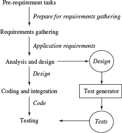
Figure 5.1 Design and test generation in a software development process. A design is an artifact generated in the Analysis and Design phase. This artifact becomes an input to the Test Generator algorithm that generates tests for input to the code during testing.

The design is often subjected to test prior to its input to the coding step. Simulation tools are used to check if the state transitions depicted in the statecharts do conform to the application requirements. Once the design has passed the test, it serves as an input to the coding step. Once the individual modules of the application have been coded, successfully tested, and debugged, they are integrated into an application and another test step is executed. This test step is known by various names such as system test and design verification test. In any case, the test cases against which the application is run can be derived from a variety of sources, design being one.

In this chapter, we show how a design can serve as source of tests that are used to test the application itself. As shown in Figure 5.1, the design generated at the end of the analysis and design phase serves as an input to a test generation procedure. This test generation procedure generates a number of tests that serve as inputs to the code in the test phase. Note that though Figure 5.1 seems to imply that the test generation procedure is applied to the entire design, this is not necessarily true; tests can be generated using portions of the design.

 

We introduce several test generation procedures to derive tests from FSMs. An FSM offers a simple way to model state-based behavior of applications. The statechart is a rich extension of the FSM and needs to be handled differently when used as an input to a test generation algorithm. The Petri net is a useful formalism to express concurrency and timing and leads to yet another set of algorithms for generating tests. All test generation methods described in this chapter can be automated, though only some have been integrated into commercial test tools.

There exist several algorithms that take an FSM and some attributes of its implementation as inputs to generate tests. Note that the FSM serves as a source for test generation and is not the item under test. It is the implementation of the FSM that is under test. Such an implementation is also known as Implementation Under Test and abbreviated as IUT. For example, an FSM may represent a model of a communication protocol while an IUT is its implementation. The tests generated by the algorithms introduced in this chapter are inputs to the IUT to determine if the IUT behavior conforms to the requirements.

The following methods are introduced in this chapter: the W-method, the transition tour method, the distinguishing sequence method, the unique input/output method, and the partial W-method. In Section 5.9, we compare the various methods introduced. Before proceeding to describe the test generation procedures, we introduce a fault model for FSMs, the characterization set of an FSM, and a procedure to generate this set. The characterization set is useful in understanding and implementing the test generation methods introduced subsequently.

5.2  Finite State Machines

Many devices used in daily life contain embedded computers. For example, an automobile has several embedded computers to perform various tasks, engine control being one example. Another example is a computer inside a toy for processing inputs and generating audible and visual responses. Such devices are also known as embedded systems. An embedded system can be as simple as a child’s musical keyboard or as complex as the flight controller in an aircraft. In any case, an embedded system contains one or more computers for processing inputs.

An embedded computer often receives inputs from its environment and responds with appropriate actions. While doing so, it moves from one state to another. The response of an embedded system to its inputs depends on its current state. It is this behavior of an embedded system in response to inputs that is often modeled by an FSM. Relatively simpler systems, such as protocols, are modeled using FSMs. More complex systems, such as the engine controller of an aircraft, are modeled using statecharts which can be considered as a generalization of FSMs. In this section, we focus on FSMs. The next example illustrates a simple model using an FSM.

 

Example 5.1   Consider a traditional table lamp that has a three-way rotary switch. When the switch is turned to one of its positions, the lamp is in the OFF state. Moving the switch clockwise to the next position moves the lamp to an ON-DIM state. Moving the switch further clockwise moves the lamp to the ON-BRIGHT state. Finally, moving the switch clockwise one more time brings the lamp back to the OFF state. The switch serves as the input device that controls the state of the lamp. The change of lamp state in response to the switch position is often illustrated using a state diagram as in Figure 5.2(a).

Our lamp has three states OFF, ON_DIM, and ON_BRIGHT, and one input. Note that the lamp switch has three distinct positions, though from a lamp user’s perspective the switch can only be turned clockwise to its next position. Thus, “turning the switch one notch clockwise” is the only input. Suppose that the switch also can be moved counterclockwise. In this latter case, the lamp has two inputs one corresponding to the clockwise motion and the other to the counterclockwise motion. The number of distinct states of the lamp remains three but the state diagram is now as in Figure 5.2(b).

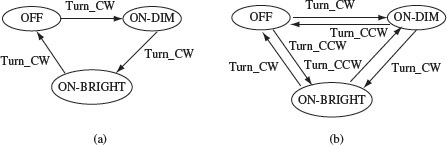
Figure 5.2 Change of lamp state in response to the movement of a switch. (a) Switch can only move one notch clockwise (CW). (b) Switch can move one notch clockwise and counterclockwise (CCW).

In the above example, we have modeled the table lamp in terms of its states, inputs, and transitions. In most practical embedded systems, the application of an input might cause the system to perform an action in addition to performing a state transition. The action might be as trivial as “do nothing” and simply move to another state, or a complex function might be executed. The next example illustrates one such system.

 

Example 5.2   Consider a machine that takes a sequence of one or more unsigned decimal digits as input and converts the sequence to an equivalent integer. For example, if the sequence of digits input is 3, 2, and 1, then the output of the machine is 321. We assume that the end of the input digit sequence is indicated by the asterisk (*) character. We shall refer to this machine as the DIGDEC machine. The state diagram of DIGDEC is shown in Figure 5.3.

The DIGDEC machine can be in any one of three states. It begins its operation in state q₀. Upon receiving the first digit, denoted by d in the figure, it invokes the function INIT to initialize variable num to d. In addition, the machine moves to state q₁ after performing the INIT operation. In q₁ DIGDEC can receive a digit or an end-of-input character which in our case is the asterisk. If it receives a digit, it updates num to 10 * num + d and remains in state q₁. Upon receiving an asterisk the machine executes the OUT operation to output the current value of num and moves to state q₂. Notice the double circle around state q₂. Often, such a double circle is used to indicate a final state of an FSM.

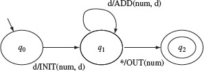
Figure 5.3 State diagram of the DIGDEC machine that converts sequence of decimal digits to an equivalent decimal number.

Historically, FSMs that do not associate any action with a transition are known as Moore machines. In Moore machines, actions depend on the current state. In contrast, FSMs that do associate actions with each state transition are known as Mealy machines. In this book, we are concerned with Mealy machines. In either case, an FSM consists of a finite set of states, a set of inputs, a start state, and a transition function which can be defined using the state diagram. In addition, a Mealy machine has a finite set of outputs. A formal definition of a Mealy machine follows.

 

Finite State Machine:

 

A finite state machine is a six tuple (X, Y, Q, q₀, δ, O) where

• X is a finite set of input symbols also known as the input alphabet,
• Y is a finite set of output symbols also known as the output alphabet,
• Q is a finite set of states,
• q₀ ϵ Q is the initial state,
• δ : Q × X → Q is a next-state or state transition function, and
• O : Q × X → Y is an output function.

In some variants of FSM more than one state could be specified as an initial state. Also, sometimes, it is convenient to add F ⊆ Q as a set of final or accepting states while specifying an FSM. The notion of accepting states is useful when an FSM is used as an automaton to recognize a language. Also note that the definition of the transition function δ implies that for any state q_i in Q, there is at most one next state. Such FSMs are also known as deterministic FSMs. In this book, we are concerned only with deterministic FSMs. The state transition function for non-deterministic FSMs is defined as

 

 

which implies that such an FSM can have more than one possible transition out of a state on the same symbol. Non-deterministic FSMs are usually abbreviated as NFSM or NDFSM or simply as NFA for Non-deterministic Finite Automata.

Figure 5.4 Multiple labels for an edge connecting two states in an FSM.

The state transition and the output functions are extended to strings as follows. Let q_i and q_j be two, possibly same, states in Q and s = a₁a₂ . . . a_n a string over the input alphabet X of length n ≥ 0. δ(q_i, s) = q_j if δ(q_i, a₁) = q_k and δ(q_k, a₂a₃ . . . a_n) = q_j. The output function is extended similarly. Thus, O(q_i, s) = O(q_i, a₁) · O(δ(q_i, a₁), a₂, a₃, . . . , a_n). Also, δ(q_i, ϵ) = q_i and O(q_i, ϵ) = ϵ.

 

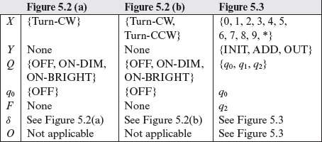
Table 5.1 contains a formal description of the state and output functions of FSMs given in Figures 5.2 and 5.3. There is no output function for the table lamp. Note that the state transition function δ and the output function O can be defined by a state diagram as in Figures 5.2 and 5.3. Thus, for example, from Figure 5.2(a), we can derive δ(OFF, Turn_CW) = ON_DIM. As an example of the output function, we get O = INIT(num, 0) from Figure 5.3.

 

Table 5.1 Formal description of three FSMs from Figures 5.2 and 5.3.

A state diagram is a directed graph that contains nodes representing states and edges representing state transitions and output functions. Each node is labeled with the state it represents. Each directed edge in a state diagram connects two states.

Each edge is labeled i/o where i denotes an input symbol that belongs to the input alphabet X and ο denotes an output symbol that belongs to the output alphabet Y . i is also known as the input portion of the edge and ο its output portion. Both i and ο might be abbreviations. As an example, the edge connecting states q₀ and q₁ in Figure 5.3 is labeled d/INIT(num, d) where d is an abbreviation for any digit from 0 to 9 and INIT(num, d) is an action.

 

Multiple labels can also be assigned to an edge. For example, the label i₁/o₁ and i₂/o₂ associated with an edge that connects two states q_i and q_j implies that the FSM can move from q_i to q_j upon receiving either i₁ or i₂. Further, the FSM outputs o₁ if it receives input i₁ and outputs o₂ if it receives o₂. The transition and the output functions can also be defined in tabular form as explained in Section 5.2.2.

5.2.1  Excitation using an input sequence

In most practical situations, an implementation of an FSM is excited using a sequence of input symbols drawn from its input alphabet. For example, suppose that the table lamp whose state diagram is in Figure 5.2(b) is in state ON-BRIGHT and receives the input sequence r where

 

r = Turn_CCW Turn_CCW Turn_CW

 

Using the transition function in Figure 5.2(b), it is easy to verify that the sequence s will move the lamp from state ON_BRIGHT to state ON_DIM. This state transition can also be expressed as a sequence of transitions given below.

 

δ(ON_BRIGHT, Turn_CCW) = ON_DIM

δ(ON_DIM, Turn_CCW) = OFF

δ(OFF, Turn_CW) = ON_DIM

 

For brevity, we will use the notation δ(q_k, z) = q_j to indicate that an input sequence z of length one or more moves an FSM from state q_k to state q_j. Using this notation, we can write δ(ON_BRIGHT, r) = ON_DIM for the state diagram in Figure 5.2(b).

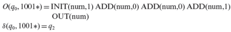
We will use a similar abbreviation for the output function O. For example, when excited by the input sequence 1001*, the DIGDEC machine ends up in state q₂ after executing the following sequence of actions and state transitions:

 

O(q₀, 1) = INIT(num,1), δ(q₀, 1) = q₁

O(q₁, 0) = ADD(num,0), δ(q₁, 0) = q₁

O(q₁, 0) = ADD(num,0), δ(q₁, 0) = q₁

O(q₁, 1) = ADD(num,1), δ(q₁, 1) = q₁

O(q₁, *) = OUT(num), δ(q₁, *) = q₂

 

Once again, for brevity, we will use the notation O(q, r) to indicate the action sequence executed by the FSM on input r when starting in state q. We also assume that a machine remains in its current state when excited with an empty sequence. Thus, δ(q, ϵ) = q. Using the abbreviation for state transitions, we can express the above action and transition sequence as follows

5.2.2  Tabular representation

A table is often used as an alternative to the state diagram to represent the state transition function δ and the output function O. The table consists of two sub-tables that consist of one or more columns each. The leftmost sub-table is the output or the action sub-table. The rows are labeled by the states of the FSM. The rightmost sub-table is the next state sub-table. The output sub-table, that corresponds to the output function O, is labeled by the elements of the input alphabet X. The next state sub-table, that corresponds to the transition function δ, is also labeled by elements of the input alphabet. The entries in the output sub-table indicate the actions taken by the FSM for a single input received in a given state. The entries in the next state sub-table indicate the state to which the FSM moves for a given input and in a given current state. The next example illustrates how the output and transition functions can be represented in a table.

 

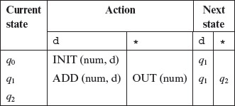
Example 5.3   The table given below shows how to represent functions δ and Ο for the DIGDEC machine. In this table, the column labeled “Action” defines the output function by listing the actions taken by the DIGDEC machine for various inputs. Sometimes, this column is also labeled as “Output” to indicate that the FSM generates an output symbol when it takes a transition. The column labeled “Next State” defines the transition function by listing the next state of the DIGDEC machine in response to an input. Empty entries in the table should be considered as undefined. However, in certain practical situations, the empty entries correspond to an “error” action. Note that in the table below we have used the abbreviation d for the ten digits, 0 through 9.

5.2.3  Properties of FSM

FSMs can be characterized by one or more of several properties. Some of the properties found useful in test generation are given below. We shall use these properties later while explaining algorithms for test generation.

 

Completely specified FSM: An FSM Μ is said to be completely specified if from each state in Μ there exists a transition for each input symbol. The machine described in Example 5.1 with state diagram in Figure 5.2(a) is completely specified as there is only one input symbol and each state has a transition corresponding to this input symbol. Similarly, the machine with state diagram shown in Figure 5.2(b) is also completely specified as each state has transitions corresponding to each of the two input symbols. The DIGDEC machine in Example 5.2 is not completely specified as state q₀ does not have any transition corresponding to an asterisk and state q₂ has no outgoing transitions.

 

Strongly connected: An FSM Μ is considered strongly connected if for each pair of states (q_i, q_j), there exists an input sequence that takes Μ from state q_i to q_j. It is easy to verify that the machine in Example 5.1 is strongly connected. The DIGIDEC machine in Example 5.2 is not strongly connected as it is impossible to move from state q₂ to q₀, from q₂ to q₁, and from q₁ to q₀. In a strongly connected FSM, given some state q_i ≠ q₀, one can find an input sequence s ϵ X* that takes the machine from its initial state to q_i. We therefore say that in a strongly connected FSM, every state is reachable from the initial state.

 

V-equivalence: Let and be two FSMs. Let V denote a set of non-empty strings over the input alphabet X, i.e. V ⊆ X⁺. Let q_i and q_j, i ≠ j, be the states of machines M₁ and M₂, respectively. States q_i and q_j are considered V-equivalent if O₁(q_i, s) = O₂(q_j, s) for all s ϵ V. Stated differently, states q_i and q_j are considered V-equivalent if M₁ and M₂, when excited in states q_i and q_j, respectively, yield identical output sequences. States q_i and q_j are said to be equivalent if O₁(q_i, s) = O₂(q_j, s) for any set V. If q_i and q_j are not equivalent, then they are said to be distinguishable. This definition of equivalence also applies to states within a machine. Thus, machines M₁ and M₂ could be the same machine.

Machine equivalence: Machines M₁ and M₂ are said to be equivalent if (a) for each state σ in M₁, there exists a state σ′ in M₂ such that σ and σ′ are equivalent and (b) for each state σ in M₂, there exists a state σ′ in M₁ such that σ and σ′ are equivalent. Machines that are not equivalent are considered distinguishable. If M₁ and M₂ are strongly connected, then they are equivalent if their respective initial states, are equivalent. We write M₁ = M₂ if machines M₁ and M₂ are equivalent and M₁ ≠ M₂ when they are distinguishable. Similarly, we write q_i = q_j when states q_i and q_j are equivalent and q_i ≠ q_j if they are distinguishable.

 

k-equivalence: Let and be two FSMs. States q_i ϵ Q₁ and q_j ϵ Q₂ are considered k-equivalent if when excited by any input of length k, yield identical output sequences. States that are not k-equivalent are considered k-distinguishable. Once again, M₁ and M₂ may be the same machines implying that k-distinguishability applies to any pair of states of an FSM. It is also easy to see that if two states are k-distinguishable for any k > 0, then they are also distinguishable for any n > k. If M₁ and M₂ are not k-distinguishable, then they are said to be k-equivalent.

 

Minimal machine: An FSM Μ is considered minimal if the number of states in Μ is less than or equal to any other FSM equivalent to M.

 

Example 5.4   Consider the DIGDEC machine in Figure 5.3. This machine is not completely specified. However, it is often the case that certain erroneous transitions are not indicated in the state diagram. A modified version of the DIGDEC machine appears in Figure 5.5. Here, we have labeled explicitly the error transitions by the output function ERROR( ).

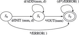
Figure 5.5 State diagram of a completely specified machine for converting a sequence of one or more decimal digits to their decimal number equivalent. d|* refers to digit or any other character.

5.3  Conformance Testing

The term conformance testing is used during the testing of communication protocols. An implementation of a communication protocol is said to conform to its specification if the implementation passes a collection of tests derived from the specification. In this chapter, we introduce techniques for generating tests to test an implementation for conformance testing of a protocol modeled as an FSM. Note that the term conformance testing applies equally well to the testing of any implementation that corresponds to its specification, regardless of whether or not the implementation is that of a communication protocol.

 

Communication protocols are used in a variety of situations. For example, a common use of protocols is in public data networks. These networks use access protocols such as the X.25 which is a protocol standard for wide area network communications. The Alternating Bit Protocol (ABP) is another example of a protocol used in the connection-less transmission of messages from a transmitter to a receiver. Musical instruments such as synthesizers and electronic pianos use the MIDI (Musical Instrument Digital Interface) protocol to communicate amongst themselves and a computer. These are just a few examples of a large variety of communication protocols that exist and new ones are often under construction.

 A protocol can be specified in a variety of ways. For example, it could be specified informally in textual form. It could also be specified more formally using an FSM, a visual notation such as a statechart, and using languages such as LOTOS (Language of Temporal Ordering Specification), Estelle, and SDL. In any case, the specification serves as a source for implementers and also for automatic code generators. As shown in Figure 5.6, an implementation of a protocol consists of a control portion and a data portion. The control portion captures the transitions in the protocol from one state to another. It is often modeled as an FSM. The data portion maintains information needed for the correct behavior. This includes counters and other variables that hold data. The data portion is modeled as a collection of program modules or segments.

 

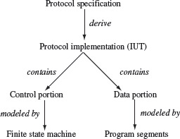
Figure 5.6 Relationship amongst protocol specification, implementation, and models.

Testing an implementation of a protocol involves testing both the control and data portions. The implementation under test is often referred to as IUT. In this chapter, we are concerned with testing the control portion of an IUT. Techniques for testing the data portion of the IUT are described in other chapters. Testing the control portion of an IUT requires the generation of test cases. As shown in Figure 5.7, the IUT is tested against the generated tests. Each test is a sequence of symbols that are input to the IUT. If the IUT behaves in accordance with the specification, as determined by an oracle, then its control portion is considered equivalent to the specification. Non-conformance usually implies that the IUT has an error that needs to be fixed. Such tests of an IUT are generally effective in revealing certain types of implementation errors discussed in Section 5.4.

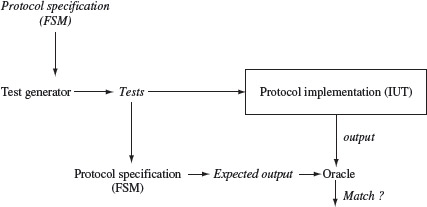
Figure 5.7 A simplified procedure for testing a protocol implementation against an FSM model. Italicized items represent data input to some procedure. Note that the model itself serves as data input to the test generator and as a procedure for deriving the expected output. 

A significant portion of this chapter is devoted to describing techniques for generating tests to test the control portion of an IUT corresponding to a formally specified design. The techniques described for testing IUTs modeled as FSMs are applicable to protocols and other requirements that can be modeled as FSMs. Most complex software systems are generally modeled using statecharts, and not FSMs. However, some of the test generation techniques described in this chapter are useful in generating tests from statecharts.

5.3.1  Reset inputs

The test methods described in this chapter often rely on the ability of a tester to reset the IUT so that it returns to its start state. Thus, given a set of test cases T = {t₁, t₂, . . . , t_n}, a test proceeds as follows:

 

1. Bring the IUT to its start state. Repeat the following steps for each test in Τ.
2. Select the next test case from Τ and apply it to the IUT. Observe the behavior of the IUT and compare it against the expected behavior as shown in Figure 5.7. The IUT is said to have failed if it generates an output different from the expected output.
3. Bring the IUT back to its start state by applying the reset input and repeat the above step but with the next test input.

It is usually assumed that the application of the reset input generates a null output. Thus, for the purpose of testing an IUT against its control specification FSM Μ = (X, Y, Q, q₁, δ, O), the input and output alphabets are augmented as follows:

X = X ∪ {Re}

Y = Y ∪ {null}

where Re denotes the reset input and null the corresponding output.

 While testing a software implementation against its design, a reset input might require executing the implementation from the beginning, i.e. restarting the implementation, manually or automatically via, for example, a script. However, in situations where the implementation causes side effects, such as writing to a file or sending a message over a network, bringing the implementation to its start state might be a non-trivial task if its behavior depends on the state of the environment. While testing continuously running programs, such as network servers, the application of a reset input does imply bringing the server to its initial state but not necessarily shutting it down and restarting.

 

The transitions corresponding to the reset input are generally not shown in the state diagram. In a sense, these are hidden transitions that are allowed during the execution of the implementation. When necessary, these transitions could be shown explicitly as in Figure 5.8.

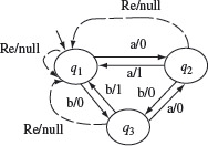
Figure 5.8 Transitions corresponding to reset (Re) inputs. 

Example 5.5   Consider the test of an application that resides inside a microwave oven. Suppose that one test, say t₁, corresponds to testing the “set clock time” functions. Another test, say t₂, corresponds to the heating ability of the oven under “low power” setting. Finally, the third test t₃ tests the ability of the oven under “high power” setting. In its start state, the oven has electrical power applied and is ready to receive commands from its keypad. We assume that the clock time setting is not a component of the start state. This implies that the current time on the clock, e.g. 1:15 pm or 2:09 am, does not have any effect on the state of the oven.

It seems obvious that the three tests mentioned above can be executed in any sequence. Further, once a test is completed and the oven application, and the oven, does not fail, the oven will be in its start state and hence no explicit reset input is required prior to executing the next test.

However, the scenario mentioned above might change after the application of, for example, t₂, if there is an error in the application under test or in the hardware that receives control commands from the application under test. For example, the application of t₂ is expected to start the oven’s heating process. However, due to some hardware or software error, this might not happen and the oven application might enter a loop waiting to receive a “task completed” confirmation signal from the hardware. In this case, tests t₃ or t₁ cannot be applied unless the oven control software and hardware are reset to their start state.

It is due to situations such as the one described in the previous example that require the availability of a reset input to bring the IUT under test to its start state. Bringing the IUT to its start state gets it ready to receive the next test input.

5.3.2  The testing problem

There are several ways to express the design of a system or a subsystem. FSM, statecharts, and Petri Nets are some of the formalisms to express various aspects of a design. Protocols, for example, are often expressed as FSMs. Software designs are expressed using statecharts. Petri nets are often used to express aspects of designs that relate to concurrency and timing. The design is used as a source for the generation of tests that are used subsequently to test the IUT for conformance to the design.

 Let Μ be a formal representation of a design. As above, this could be an FSM, a statechart, or a Petri net. Other formalisms are possible too. Let R denote the requirements that led to M. R may be for a communication protocol, an embedded system such as the automobile engine or a heart pacemaker. Often, both R and Μ are used as the basis for the generation of tests and to determine the expected output as shown in Figure 5.7. In this chapter, we are concerned with the generation of tests using M.

 

The testing problem is to determine if the IUT is equivalent to M. For the FSM representation, equivalence was defined earlier. For other representations, equivalence is defined in terms of the input/output behavior of the IUT and M. As mentioned earlier, the protocol or design of interest might be implemented in hardware, software, or a combination of the two. Testing the IUT for equivalence against Μ requires executing it against a sequence of test inputs derived from Μ and comparing the observed behavior with the expected behavior as shown in Figure 5.7. Generation of tests from a formal representation of the design and their evaluation in terms of their fault detection ability is the key subject of this chapter.

5.4  A Fault Model

Given a set of requirements R, one often constructs a design from the requirements. An FSM is one possible representation of the design. Let M_d be a design intended to meet the requirements in R. Sometimes, M_d is referred to as a specification that guides the implementation. M_d is implemented in hardware or software. Let M_i denote an implementation that is intended to meet the requirements in R and has been derived using M_d. Note that, in practice, M_i is unlikely to be an exact analog of M_d. In embedded real-time systems and communications protocols, it is often the case that M_i is a computer program that uses variables and operations not modeled in M_d. Thus, one could consider M_d as a finite state model of M_i.

The problem in testing is to determine whether or not M_i conforms to R. To do so, one tests M_i using a variety of inputs and checks for the correctness of the behavior of M_i with respect to R. The design M_d can be useful in generating a set Τ of tests for M_i. Tests so generated are also known as black-box tests, because they have been generated with reference to M_d and not M_i. Given T, one tests M_i against each test t ϵ Τ and compares the behavior of M_i with the expected behavior given by exciting M_d in the initial state with test t.

 

In an ideal situation, one would like to ensure that any error in M_i is revealed by testing it against some test t ϵ Τ derived from M_d. One reason why this is not feasible is that the number of possible implementations of a design M_d is infinite. This gives rise to the possibility of a large variety of errors one could introduce in M_i. In the face of this reality, a fault model has been proposed. This fault model defines a small set of possible fault types that can occur in M_i. Given a fault model, the goal is to generate a test set Τ from a design M_d. Any fault in M_i of the type in the fault model, is guaranteed to be revealed when tested against Τ.

A widely used fault model for FSMs is shown in Figure 5.9. This figure illustrates four fault categories.

• Operation error: Any error in the output generated upon a transition is an operation error. This is illustrated by machines Μ and M₁ in Figure 5.9 where FSM M₁ generates an output 0, instead of a 1, when symbol a is input in state q₀. More formally, an operation error implies that for some state q_i in Μ and some input symbol s, O(q_i, s) is incorrect.

   

  A fault model for testing using FSMs includes four types of errors: operation error, transfer error, extra state error, and missing state error. An operation error implies an incorrect output function. A transfer error implies an incorrect state transition function.

• Transfer error: Any error in the transition from one state to the next is a transition error. This is illustrated by machine M₂ in Figure 5.9 where FSM M₂ moves to state q₁, instead of moving to q₀ from q₀ when symbol a is input. More formally, a transfer error implies that for some state q_i in Μ and some input symbol s, δ(q_i, x) is incorrect.
• Extra state error: An extra state may be introduced in the implementation. In Figure 5.9, machine M₃ has q₂ as the extra state when compared with the state set of machine M. However, an extra state may or may not be an error. For example, in Figure 5.10, machine Μ represents the correct design. Machines M₁ and M₂ have one extra state each. However, M₁ is an erroneous design but M₂ is not. This is because M₂ is actually equivalent to Μ even though it has an extra state.
  

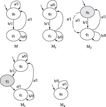
  Figure 5.9 Machine Μ represents the correct design. Machines M₁, M₂, M₃, and M₄ each contain an error.

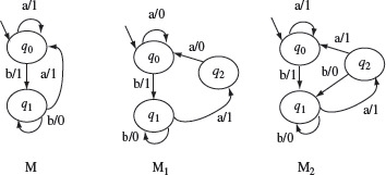
Figure 5.10 Machine Μ represents the correct design. Machines M₁ and M₂ each have an extra state. However, M₁ is erroneous and M₂ is equivalent to M. 

• Missing state error: A missing state is another type of error. We note from Figure 5.9 that machine M₄ has q₁ missing when compared with machine M. Given that the machine representing the correct design is minimal and complete, a missing state implies an error in the IUT.

The above fault model is generally used to evaluate a method for generating tests from a given FSM. The faults indicated above are also known collectively as sequencing faults or sequencing errors. It may be noted that a given implementation could have more than one error of the same type. Other possibilities, such as two errors one each of a different type, also exist.

5.4.1  Mutants of FSMs

As mentioned earlier, given a design M_d, one could construct many correct and incorrect implementations. Let I(M_d) denote the set of all possible implementations of M_d. In order to make I finite, we assume that any implementation in I(M_d) differs from M_d in known ways. One way to distinguish an implementation from its specification is through the use of mutants. A mutant of M_d is an FSM obtained by introducing one or more errors one or more times. We assume that the errors introduced belong to the fault model described earlier. Using this method, we see in Figure 5.9 four mutants M₁, M₂, M₃, and M₄ of machine M. More complex mutants can also be obtained by introducing more than one error in a machine. Figure 5.11 shows two such mutants of machine Μ of Figure 5.9.

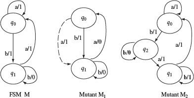
Figure 5.11 Two mutants of machine M. Mutant M₁ is obtained by introducing into Μ one operation error in state q₁ and one transfer error in state q₀ for input a. Mutant M₂ has been obtained by introducing an extra state q₂ in machine Μ and an operation error in state q₁, on input b. 

Note that a mutant may be equivalent to M_d implying that the output behaviors of M_d and the mutant are identical on all possible inputs. Given a test set T, we say that a mutant is distinguished from M_d by a test t ϵ T, if the output sequence generated by the mutant is different from that generated by M_d when excited with t in their respective initial states. In this case, we also say that Τ distinguishes the mutant.

Using the idea of mutation, one can construct a finite set of possible implementations of a given specification M_d. Of course, this requires that some constraints are placed on the process of mutation, i.e. on how the errors are introduced. We caution the reader that the technique of testing software using program mutation is different from the use of mutation described here. This difference is discussed in Chapter 8. The next example illustrates how to obtain one set of possible implementations.

 

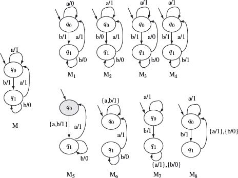
Example 5.6   Let Μ shown in Figure 5.12 denote the correct design. Suppose that we are allowed to introduce only one error at a time in M. This generates four mutants M₁, M₂, M₃, and M₄ shown in Figure 5.12 obtained by introducing an operation error. Considering that each state has two transitions, we get four additional mutants M₅, M₆, M₇, and M₈ by introducing the transfer error.

Figure 5.12 Eight first-order mutants of Μ generated by introducing operation and transfer errors. Mutants M₁, M₂, M₃, and M₄ are generated by introducing operation errors in M. Mutants M₅, M₆, M₇, and M₈ are generated by introducing transfer errors in M.

Introducing an additional state to create a mutant is more complex. First, we assume that only one extra state can be added to the FSM. However, there are several ways in which this state can interact with the existing states in the machine. This extra state can have two transitions that can be specified in 36 different ways depending on the tail state of the transition and the associated output function. We delegate to Exercise 5.10 the task of creating all the mutants of Μ by introducing an extra state.

Removing a state can be done in only two ways: remove q₀ or remove q₁. This generates two mutants. In general, this could be more complex when the number of states is greater than three. Removing a state will require the redirection of transitions and hence the number of mutants generated will be more than the number of states in the correct design.

Any non-empty test starting with symbol a distinguishes Μ from M₁. Mutant M₂ is distinguished from Μ by the input sequence ab. Note that when excited with ab, Μ outputs the string 11, whereas M₂ outputs the string 10. Input ab also distinguishes M₅ from M. The complete set of distinguishing inputs can be found using the W-method described in Section 5.6.

5.4.2  Fault coverage

One way to determine the “goodness” of a test set is to compute how many errors it reveals in a given implementation M_i. A test set that can reveal all errors in M_i is considered superior to one that fails to reveal one or more errors. Methods for the generation of test sets are often evaluated based on their fault coverage. The fault coverage of a test set is measured as a fraction between 0 and 1 and with respect to a given design specification. We give a formal definition of fault coverage in the following where the fault model presented earlier is assumed to generate the mutants.

 

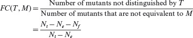
N_t: Total number of first-order mutants of the machine Μ used for generating tests. This is also the same as |I(M)|.

N_e: Number of mutants that are equivalent to M.

N_f : Number of mutants that are distinguished by test set Τ generated using some test generation method. Recall that these are the faulty mutants as no input in Τ is able to distinguish these mutants.

N_l: Number of mutants that are not distinguished by Τ.

The fault coverage of a test suite Τ with respect to a design M, and an implementation set I(M), is denoted by FC(T, M) and computed as follows.

In Section 5.9, we will see how FC can be used to evaluate the goodness of various methods to generate tests from FSMs. Next, we introduce the characterization set, and its computation, useful in various methods for generating tests from FSMs.