
9
Test Selection, Minimization, and Prioritization for Regression Testing
CONTENTS
9.1 What is regression testing?
9.3 Regression test selection: the problem
9.4 Selecting regression tests
9.5 Test selection using execution trace
9.6 Test selection using dynamic slicing
The purpose of this chapter is to introduce techniques for the selection, minimization, and prioritization of tests for regression testing. The source Τ from which tests are selected is likely derived using a combination of black-box and white-box techniques and used for system or component testing. However, when this system or component is modified, for whatever reason, one might be able to retest it using only a subset of Τ and ensure that despite the changes, the existing unchanged code continues to function as desired. A sample of techniques for the selection, minimization, and prioritization of this subset are presented in this chapter.
9.1 What Is Regression Testing?
The word regress means to return to a previous, usually worse, state. Regression testing refers to that portion of the test cycle in which a program Ρ' is tested to ensure that not only does the newly added or modified code behaves correctly, but also that code carried over unchanged from the previous version Ρ continues to behave correctly. Thus regression testing is useful, and needed, whenever a new version of a program is obtained by modifying an existing version.
A program that is modified for reasons such as correction, addition of features, etc., is often retested to ensure that the unchanged parts of the program continue to work correctly. Such testing is commonly referred to as “regression testing.”
Regression testing is sometimes referred to as “program revalidation.” The term “corrective regression testing” refers to regression testing of a program obtained by making corrections to the previous versions. Another term “progressive regression testing” refers to regression testing of a program obtained by adding new features. A typical regression testing scenario often includes both corrective and progressive regression testing. In any case, techniques described in this chapter are applicable to both types of regression testing.
To understand the process of regression testing, let us examine a development cycle exhibited in Figure 9.1. The figure shows a highly simplified develop-test-release process for program P, referred to as Version 1. While Ρ is in use, there might be a need to add new features, remove any reported errors, and rewrite some code to improve performance. Such modifications lead to P′, referred to as Version 2. This modified version must be tested for any new functionality (step 5 in the figure). However, when making modifications to Ρ the developers might mistakenly add or remove code that causes the existing and unchanged functionality from Ρ to stop behaving as desired. One performs regression testing (step 6) to ensure that any malfunction of the existing code is detected and repaired prior to the release of P′.
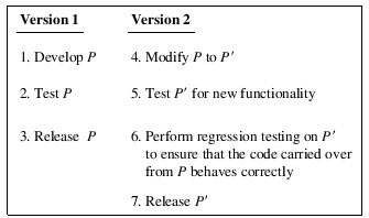
Figure 9.1 Two phases of product development and maintenance. Version 1 (P) is developed, tested, and released in the first phase. In the next phase, Version 2 (P′) is obtained by modifying Version 1.
It should be obvious from the above description that regression testing can be applied in each phase of software development. For example, during unit testing, when a given unit such as a class is modified by adding new methods, one needs to perform regression testing to ensure that methods not modified continue to work as required. Certainly, regression testing is redundant in cases where the developer can demonstrate through suitable arguments that the methods added can have no effect on the existing methods.
Regression testing may occur in any phase of software development. Thus, it might not be a distinct test phase by itself.
Regression testing is also needed when a subsystem is modified to generate a new version of an application. When one or more components of an application are modified, the entire application must also be subject to regression testing. In some cases regression testing might be needed when the underlying hardware changes. In this case, regression testing is performed despite any change in the software.
In the remainder of this chapter you will find various techniques for regression testing. It is important to note that some techniques introduced in this chapter, while sophisticated, might not be applicable in certain environments while absolutely necessary in others. Hence, it is important to understand not only the technique for regression testing but also its strengths and limitations.
9.2 Regression Test Process
A regression test process is exhibited in Figure 9.2. The process assumes that P′ is available for regression testing. There is usually a long series of tasks that lead to P′ from P. These tasks, not shown in Figure 9.2, include creation of one or more modification requests and the actual modification of the design and the code. A modification request might lead to a simple error fix, or to a complex redesign and coding of a component of P. In any case, regression testing is recommended after Ρ has been modified and any newly added functionality tested and found correct.
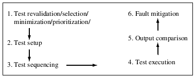
Figure 9.2 A subset of tasks in regression testing.
Regression testing becomes necessary after a program is changed due to modification requests. Such testing ensures that the changes made do not affect the correctness of other parts of the program.
The tasks in Figure 9.2 are shown as if they occur in the given sequence. This is not necessarily true and other sequencings are possible. Several of the tasks shown can be completed while Ρ is being modified to P′. It is important to note that except in some cases, for test selection, all tasks shown in the figure are performed in almost all phases of testing and are not specific to regression testing.
9.2.1 Revalidation, selection, minimization, and prioritization
While it would be ideal to test P′ against all tests developed for P, this might not be possible for several reasons. For example, there might not be sufficient time available to run all tests. Also, some tests for Ρ might become invalid for P′ due to reasons such as a change in the input data and its format for one or more features. In yet another scenario, the inputs specified in some tests might remain valid for P′ but the expected output might not. These are some reasons that necessitate Step 1 in Figure 9.2.
A brute force regression test might run all tests for the original program Ρ against the modified program P′. However, for several reasons, doing so might not be feasible or desirable.
Test revalidation refers to the task of checking which tests for Ρ remain valid for P′. Revalidation is necessary to ensure that only tests that are applicable to P′ are used during regression testing.
Test selection can be interpreted in several ways. Validated tests might be redundant in that they do not traverse any of the modified portions in P′. The identification of tests that traverse modified portions of P′ is often referred to as test selection and sometimes as the regression test selection (RTS) problem. However, note that both test minimization and prioritization described next are also techniques for test selection.
Prior to executing a modified program against the test cases used in its previous incarnation, one needs to ensure that these tests are valid. A valid test is one that will test, as desired, a feature in the modified program.
Test minimization discards tests seemingly redundant with respect to some criteria. For example, if both t1 and t2 test function f in Ρ then one might decide to discard t2 in favor of t1. The purpose of minimization is to reduce the number of tests to execute for regression testing.
Test prioritization refers to the task of prioritizing tests based on some criteria. A set of prioritized tests becomes useful when only a subset of tests can be executed due to resource constraints. Test selection can be achieved by selecting a few tests from a prioritized list. However, several other methods for test selection are available as discussed later in this chapter. Revalidation, followed by selection, minimization, and prioritization is one possible sequence to execute these tasks.
The regression test selection problem is to identify tests to be run for regression testing of a modified program. Test minimization and test prioritization are two techniques for regression test selection.
Example 9.1 A Web service is a program that can be used by another program over the Web. Consider a Web service named ZC, short for ZipCode. The initial version of ZC provides two services: ZtoC and ZtoA. Service ZtoC inputs a zip code and returns a list of cities and the corresponding state while ZtoA inputs a zip code and returns the corresponding area code. We assume that while the ZipCode service can be used over the Web from wherever an Internet connection is available, it serves only the United States.
Let us suppose that ZC has been modified to ZC’ as follows. First, a user can select from a list of countries and supply the zip code to obtain the corresponding city in that country. This modification is made only to the ZtoC function while ZtoA remains unchanged. Note that the term “zip code” is not universal. For example, in India, the equivalent term is “pin code” which is 6-digits long as compared to the 5-digit zip code used in the United States. Second, a new service named ZtoT has been added which inputs a country and a zip code and returns the corresponding time zone.
Consider the following two tests (only inputs specified) used for testing ZC:
t1: <service=ZtoC, zip=47906>
t2: <service=ZtoA, zip=47906>
A simple examination of the two tests reveals that test t1 is not valid for ZC’ as it does not list the required country field. Test t2 is valid as we have made no change to ZtoA. Thus we need to either discard t1 and replace it by a new test for the modified ZtoC or simply modify t1 appropriately. We prefer to modify and hence our validated regression test suite for ZC’ is
t1: <country=USA, service=ZtoC, zip=47906>
t2: <service=ZtoA, zip=47906>
Note that testing ZC’ requires additional tests to test the ZtoT service. However, we need only the two tests listed above for regression testing. To keep this example short, we have listed only a few tests for ZC. In practice one would develop a much larger suite of tests for ZC which will then be the source of regression tests for ZC’.
9.2.2 Test setup
Test setup refers to the process by which the application under test is placed in its intended, or simulated, environment ready to receive data and able to transfer any desired output information. This process could be as simple as double clicking on the application icon to launch it for testing and as complex as setting up the entire special purpose hardware and monitoring equipment and initializing the environment before the test could begin. Test setup becomes even more challenging when testing embedded software such as that found in printers, cell phones, Automated Teller Machines, medical devices, and automobile engine controllers.
Note that test setup is not special to regression testing, it is also necessary during other stages of testing such as during integration or system testing. Often test setup requires the use of simulators that allow the replacement of a “real device” to be controlled by the software with its simulated version. For example, a heart simulator is used while testing a commonly used heart control device known as the pacemaker. The simulator allows the pacemaker software to be tested without having to install it inside a human body.
The test setup process and the setup itself are highly dependent on the application under test and its hardware and software environment. For example, the test setup process and the setup for an automobile engine control software is quite different from that of a cell phone. In the former one needs an engine simulator, or the actual automobile engine to be controlled, while in the latter one needs a test driver that can simulate the constantly changing environment.
9.2.3 Test sequencing
The sequence in which tests are input to an application may or may not be of concern. Test sequencing often becomes important for an application that has an internal state and is continuously running. Banking software, Web service, engine controller are examples of such applications. Sequencing requires grouping and sequencing tests to be run together. The following example illustrates the importance of test sequencing.
The sequence in which a program is executed against tests becomes important when the state of the program and that of its environment determines the program’s response to the next test case. Banking applications are one example where test sequencing becomes important.
Example 9.2 Consider a simplified banking application referred to as SATM. Application SATM maintains account balances and offers users the following functionality: login, deposit, withdraw, and exit. Data for each account are maintained in a secure database.
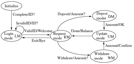
Figure 9.3 exhibits the behavior of SATM as a finite state machine. Note that the machine has six distinct states, some referred to as modes in the figure. These are labeled as Initialize, LM, RM, DM, UM, and WM. When launched, the SATM performs initialization operations, generates an “ID?” message, and moves to the LM state. If a user enters a valid ID, SATM moves to the RM state else it remains in the LM state and again requests for an ID.
Figure 9.3 State transition in a simplified banking application. Transitions are labeled as X/Y, where X indicates an input and Y the expected output. “Complete” is an internal input indicating that the application moves to the next state upon completion of operations in its current state.
While in the RM state the application expects a service request. Upon receiving a Deposit request it enters the DM state and asks for an amount to be deposited. Upon receiving an amount it generates a confirmatory message and moves to the UM state where it updates the account balance and gets back to the RM state. A similar behavior is shown for the Withdraw request. SATM exits the RM state upon receiving an Exit request.
As an example, the state transitions in a banking application require that tests be sequenced appropriately.
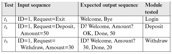
Let us now consider a set of three tests designed to test the Login, Deposit, Withdraw, and Exit features of SATM. The tests are given in the following table in the form of a test matrix. Each test requires that the application be launched fresh and the user (tester in this case) log in. We assume that the user with ID=1 begins with an account balance of 0. Test t1 checks the login module and the Exit feature, t2 the Deposit module, and t3 the Withdraw module. As you might have guessed, these tests are not sufficient for a thorough test of SATM, but they suffice to illustrate the need for test sequencing as explained next.
Now suppose that the Withdraw module has been modified to implement a change in withdrawal policy, e.g. “No more than $300 can be withdrawn on any single day.” We now have the modified SATM’ to be tested for the new functionality as well as to check if none of the existing functionality has broken. What tests should be rerun?
Assuming that no other module of SATM has been modified, one might propose that tests t1 and t2 need not be rerun. This is a risky proposition unless some formal technique is used to prove that indeed the changes made to the Withdraw module cannot affect the behavior of the remaining modules.
Let us assume that the testers are convinced that the changes in SATM will not affect any module other than Withdraw. Does this mean that we can run only t3 as a regression test? The answer is in the negative. Recall our assumption that testing of SATM begins with an account balance of 0 for the user with ID=1. Under this assumption, when run as the first test, t3 will likely fail because the expected output will not match the output generated by SATM’ (see Exercise 9.1).
The argument above leads us to conclude that we need to run test t3 after having run t2. Running t2 ensures that SATM’ is brought to the state in which we expect test t3 to be successful.
Note that the finite state machine shown in Figure 9.3 ignores the values of internal variables and databases used by SATM and SATM’. During regression as well as many other types of testing, test sequencing is often necessary to bring the application to a state where the values of internal variables, and contents of the databases used, correspond to the intention at the time of designing the tests. It is advisable that such intentions (or assumptions) be documented along with each test.
Regression tests can be executed automatically using some of the existing tools, also known as “test runners.” Nevertheless, no general purpose tool might be applicable in a given environment for the automated execution of regression tests.
9.2.4 Test execution
Once the testing infrastructure has been set up, tests selected, revalidated, and sequenced, it is time to execute them. This task is often automated using a generic or a special purpose tool. General purpose tools are available to run regression tests for applications such as Web service (see Section 9.10). However, most embedded systems, due to their unique hardware requirements, often require special purpose tools that input a test suite and automatically run the application against it in a batch mode.
The importance of a tool for test execution cannot be overemphasized. Commercial applications tend to be large and the size of the regression test suite usually increases as new versions arrive. Manual execution of regression tests might become impractical and error prone.
9.2.5 Output comparison
Each test needs verification. This is also done automatically with the help of the test execution tool that compares the generated output with the expected output. However, this might not be a simple process, especially in embedded systems. In such systems, often it is the internal state of the application, or the state of the hardware controlled by the application, that must be checked. This is one reason why generic tools that offer an oracle might not be appropriate for test verification.
Automated testing requires running a program against inputs and checking if the output is correct. The latter is the “oracle” problem. In the case of regression testing the expected test outputs might be available from the past.
One of the goals for test execution is to measure an application’s performance. For example, one might want to know how many requests per second can be processed by a Web service. In this case performance, and not functional correctness, is of interest. The test execution tool must have special features to allow such measurements.
9.3 Regression Test Selection: The Problem
Let us examine the regression testing problem with respect to Figure 9.4. Let Ρ denote Version X that has been tested using test set Τ against specification S. Let P′ be generated by modifying P. The behavior of P′ must conform to specification S′. Specifications S and S′ could be the same and P′ is the result of modifying Ρ to remove faults. S′ could also be different from S in that S′ contains all features in S and a few more, or that one of the features in S has been redefined in S′.
The regression test selection problem is to select a set of tests Τ such that the execution of the modified program P′against Τ will ensure that the functionality carried over from Ρ continues to work correctly.
The regression testing problem is to find a test set Tr on which P′ is to be tested to ensure that code that implements functionality carried over from Ρ works correctly. As shown in Figure 9.4, often Tr is a subset of Τ used for testing P.
In addition to regression testing, P′ must also be tested to ensure that the newly added code behaves correctly. This is done using a newly developed test set Td. Thus P′ is tested against T′ = Tr ∪ Td where Tr is the regression test suite and Td the development test suite intended to test any new functionality in P′. Note that we have subdivided Τ into three categories: redundant tests (Tu), obsolete tests (To), and regression tests (Tr). While Ρ is executed against the entire T, P′ is executed only against the regression set Tr and the development set Td. Tests in Τ that cause Ρ to terminate prematurely or enter into an infinite loop might be included in To or in Tr depending on their purpose.
The modified program Ρ must also be tested to ensure the newly implemented code is correct.
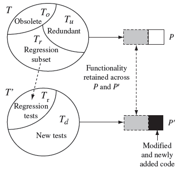
Figure 9.4 Regressing testing as a test selection problem. A subset Tr of set Τ is selected for retesting the functionality of Ρ that remains unchanged in P′.
Some tests from the previous version of the modified program might become obsolete and will not be included in the regression tests for P′.
In summary, the regression test selection problem (RTS) problem is stated as follows: Find a minimal Tr such that ∀t ϵ Tr and t′ϵ Tu ⋃ Tr, P(t) =P′(t) =⇒ P(t′)= P′(t′). In other words, the RTS problem is to find a minimal subset Tr of non-obsolete tests from Τ such that if P′ passes tests Tr then it will also pass tests in Tu. Notice that determination of Tr requires that we know the set of obsolete tests To. Obsolete tests are those no longer valid for P′ for some reason.
Identification of obsolete tests is a largely manual activity. As mentioned earlier, this activity is often referred to as test case revalidation. A test case valid for Ρ might be invalid for P′ because the input, output, or both input and output components of the test are rendered invalid by the modification to P. Such a test case either becomes obsolete and is discarded while testing P′ or is corrected and becomes a part of Tr or Tu.
Identification of obsolete tests is likely to be a manual activity.
Note that the notion of “correctness” in the above discussion is with respect to the correct functional behavior. It is possible that a solution to the RTS problem ignores a test case t on which P′ fails to meet its performance requirement whereas Ρ does. Algorithms for test selection in the remainder of this chapter ignore the performance requirement.
9.4 Selecting Regression Tests
In this section, we summarize several techniques for selecting tests for regression testing. Details of some of these techniques follow in the subsequent sections.
9.4.1 Test all
This is perhaps the simplest of all regression testing techniques. The tester is unwilling to take any risks and tests the modified program P′ against all non-obsolete tests from P. Thus, with reference to Figure 9.4, we use T′ = T – To in the test-all strategy.
A straightforward way to select regression tests is to select them all!
While the test-all strategy might be the least risky among the ones described here, it does suffer from a significant disadvantage. Suppose that P′ has been developed and the added functionality verified. Assume that one week remains to release P′. However, the test-all strategy will require at least 3-weeks for completion. In this situation one might want to use a smaller regression test suite than Τ – To. Various techniques for obtaining smaller regression test sets are discussed later in this chapter. Nevertheless, the test-all strategy combined with tools for automated regression test tools is perhaps the most widely used technique in the commercial world.
9.4.2 Random selection
Random selection of tests for regression testing is one possible method to reduce the number of tests. In this approach tests are selected randomly from the set Τ – To. The tester can decide how many tests to select depending on the level of confidence required and the available time for regression testing.
Another way to select regression tests is to select them randomly from the full set of tests.
Under the assumption that all tests are equally good in their fault detection ability, the confidence in the correctness of the unchanged code increases with an increase in the number of tests sampled and executed successfully. However, in most practical applications such an assumption is unlikely to hold. This is because some of the sampled tests might bear no relationship to the modified code while others might. This is the prime weakness of the random selection approach to regression testing. Nevertheless, random selection might turn out to be better than no regression testing at all.
9.4.3 Selecting modification traversing tests
Several regression test selection techniques aim to select a subset of Τ such that only tests that guarantee the execution of modified code and code that might be impacted by the modified code in P′ are selected while those that do not are discarded. These techniques use methods to determine the desired subset and aim at obtaining a minimal regression test suite. Techniques that obtain a minimal regression test suite without discarding any test that will traverse a modified statement are known as “safe” regression test selection techniques.
Tests that traverse the code that has been modified are good candidates to select for regression testing.
A key advantage of modification traversing tests is that when under time crunch, testers need to execute only a relatively smaller number of regression tests. Given that a “safe” technique is used, execution of such tests is likely a superior alternative to the test-all and random-selection strategies.
The sophistication of techniques to select modification traversing tests requires automation. It is impractical to apply these techniques to large commercial systems unless a tool is available that incorporates at least one safe test minimization technique. Further, while test selection appears attractive from the test effort point of view, it might not be a practical technique when tests are dependent on each other in complex ways and that this dependency cannot be incorporated in the test selection tool.
Two or more tests selected for regression might traverse exactly the same portions of the modified code. Some of these tests could be considered as redundant and excluded from the regression test. Doing so reduces the size of the regression test suite and the time to complete the test.
9.4.4 Test minimization
Suppose that Tr is a modification traversing subset of Τ. There are techniques that could further reduce the size of Tr. Such test minimization techniques aim at discarding redundant tests from Tr. A test t in Tr is considered redundant if another test u in Tr achieves the same objective as t. The objective in this context is often specified in terms of code coverage such as basic block coverage or any other form of control flow or data flow coverage. Requirements coverage is another possible objective used for test minimization.
Test minimization might not be safe in the sense that tests not selected might be actually useful in revealing errors despite the fact that they are considered redundant according to some criterion (black- or white-box).
While test minimization might lead to a significant reduction in the size of the regression test suite, it is not necessarily safe. When tests are designed carefully, minimization might discard a test case whose objective does match that used for minimization. The next example illustrates this point.
Example 9.3 Consider the following trivial program P′required to output the sum of two input integers. However, due to an error, the program outputs the difference of the two integers.
int x, y;
output (x–y)
Now suppose that Tr contains 10 tests, nine with y = 0 and one, say tnz, with non-zero values of both x and y. tnz is the only test that causes P′ to fail.
Suppose that Tr is minimized so that the basic block coverage obtained by executing P′ remains unchanged. Obviously, each of the 10 tests in Tr covers the lone basic block in P′ and therefore all but one test will be discarded by a minimization algorithm. If tnz is the one discarded then the error in P′ will not be revealed by the minimized test suite.
While the above example might seem trivial, it does point to the weakness of test minimization. Situations depicted in this example could arise in different forms in realistic applications. Hence it is recommended that minimization be carried out with caution. Tests discarded by a minimization algorithm must be reviewed carefully before being truely discarded.
9.4.5 Test prioritization
One approach to regression test selection is through test prioritization. In this approach, a suitable metric is used to rank all tests in Tr (see Figure 9.4). A test with the highest rank has the highest priority, the one with the next highest rank has the second highest priority, and so on. Prioritization does not eliminate any test from Tr. Instead, it allows the tester to decide which tests to select based on their relative priority and individual relationships based on sequencing and other requirements.
Once tests are selected for regression testing, they could be prioritized (ranked) based on one or more criteria. A ranked list of tests can be used to decide when to stop testing in case not enough resources are available to run all tests.
Example 9.4 Let R1, R2, and R3 be three requirements carried over unchanged from Ρ to P′. One approach first ranks the requirements for P′ according to their criticality. For example, a ranking might be: R2 most critical, followed by R3, and lastly R1. Any new requirements implemented in P′ but not in Ρ are not used in this ranking as they correspond to new tests in set Td as shown in Figure 9.4.
Now suppose that the regression subset Tr from Ρ is {t1, t2, t3, t4, t5} and that t1 tests R1, t2 and t3 test R2, and t4 and t5 test R3. We can now prioritize the tests in this order: t2, t3, t4, t5, t1, where t2 has the highest priority for execution and t1 the lowest. It is up to the tester to decide which tests to select for regression testing. If the tester believes that changes made to Ρ to arrive at P′ are unlikely to have any effect on code that implements R3, then tests t4 and t5 need not be executed. In case the tester has resources to run only three tests before Ρ' is to be released, then t2, t3, and t4 can be selected.
Several other more sophisticated techniques are available for test prioritization. Some of these use the amount of code covered as a metric to prioritize tests. These techniques, and others for test selection, are discussed in the following sections.
9.5 Test Selection Using Execution Trace
Let Ρ be a program containing one or more functions. Ρ has been tested against tests in Τ as shown in Figure 9.4. Ρ is modified to P′ by adding new functionality and fixing some known errors. The newly added functionality has been tested and found correct. Also, the corrections made have been tested and found adequate. Our goal now is to test P′ to ensure that the changes made do not affect the functionality carried over from P. While this could be achieved by executing P′ against all the non-obsolete tests in T, we want to select only those that are necessary to check if the modifications made do not affect functionality common to Ρ and P′.
An execution trace of a program Ρ is a sequence of program elements executed when Ρ is run against a test.
Our first technique for selecting a subset of Τ is based on the use of execution slice obtained from the execution trace of P. The technique can be split into two phases. In the first phase, Ρ is executed and the execution slice recorded for each test case in Tno = Tu ⋃ Tr (see Figure 9.4). Tno contains no obsolete test cases and hence is a candidate for full regression test. In the second phase, the modified program P′ is compared with Ρ and Tr is isolated from Tno by an analysis of the execution slice obtained in the first phase.
9.5.1 Obtaining the execution trace
Let G = (Ν, E) denote the control flow graph (CFG) of Ρ, Ν being a set of nodes and Ε a set of directed edges joining the nodes. Each node in Ν corresponds to a basic block in P. Start and End are two special elements of Ν such that Start has no ancestor and End has no descendent. For each function f in Ρ we generate a separate CFG denoted by Gf . The CFG for Ρ is also known as the main CFG and corresponds to the main function in P. All other CFGs are known as child CFGs. When necessary, we will use the notation CFG(f) to refer to the CFG of function f.
Nodes in each CFG are numbered as 1, 2, and so on with 1 being the number of the Start node. A node in a CFG is referred to by prefixing the function name to its number. For example, P.3 is node 3 in GP and f.2 node 2 in Gf .
A possible execution trace for program Ρ executed against a test is the sequence of nodes in the control flow graph of Ρ that are touched during execution.
We execute Ρ against each test in Tno. During execution against t ∊ Tno, the execution trace is recorded as trace(t). The execution trace is a sequence of nodes. We save an execution trace as a set of nodes touched during the execution of P. Such a set is also known as an execution slice of P. Start is the first node in an execution trace and End the last node. Notice that an execution trace contains nodes from functions of Ρ invoked during its execution.
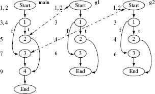
Figure 9.5 Control flow graph for function main, and its child functions g1 and g2 in Program 9.1. Line numbers corresponding to each basic block, represented as a node, are placed to the left of the corresponding node. Labels t and f indicate, respectively, true and false values of the condition in the corresponding node. Dotted lines indicate points of function calls.
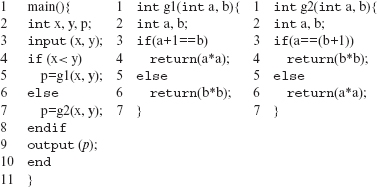
Example 9.5 Consider Program 9.1. It contains three functions: main, g1, and g2. The CFGs and child CFGs appear in Figure 9.5.
Program P9.1
Now consider the following test set:
Executing Program P9.1 against the three test cases in Τ results in the following execution traces corresponding to each test and the CFGs in Figure 9.5. We have shown the execution trace as a sequence of nodes traversed. However, a tool that generates the trace can, for the purpose of test selection, save it as a set of nodes, thereby conserving memory space.
Test (t) |
Execution trace (trace(t)) |
|---|---|
|
t1 |
main.Start, main.1, main.2, g1.Start, g1.1, g1.3, g1.End, main.2, main.4, main.End. |
|
t2 |
main.Start, main.1, main.3, g2.Start, g2.1, g2.2, g2.End, main.3, main.4, main.End. |
|
t3 |
main.Start, main.1, main.3, g2.Start, g2.1, g2.3, g2.End, main.2, main.3, main.End. |
While collecting the execution trace we assume that Ρ is started in its initial state for each test input. This might create a problem for continuously running programs, e.g. an embedded system that requires initial setup and then responds to external events that serve as test inputs. In such cases a sequence of external events serves as test case. Nevertheless, we assume that Ρ is brought into an initial state prior to the application of any external sequence of inputs that is considered a test case in Tno.
Finding an execution trace for a continuously running program might become challenging if the program needs to be brought to its initial state for each trace.
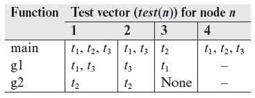
Let test(n) denote the set of tests such that each test in test(n) traversed node n at least once. Given the execution trace for each test in Tno, it is easy to find test(n) for each n ϵ N. test(n) is also known as test vector corresponding to node n.
Example 9.6 Test vectors for each node in the CFGs shown in Figure 9.5 can be found from the execution traces given in Example 9.5. These are listed in the following table. All tests traverse the Start and End nodes and hence the corresponding test vectors are not listed.
9.5.2 Selecting regression tests
This is the second phase in the selection of modification traversing regression tests. It begins when P′ is ready, has been tested and found correct in any added functionality and error fixes. The two key steps in this phase are: construct CFG and syntax trees for P′ and select tests. These two steps are described next.
Construct CFG and syntax trees: The first step in this phase is to get the CFG of P′ denoted as G′= (Ν′ ,Ε′). We now have G and G′ as the CFGs of Ρ and P′ . Recall that other than the special nodes, each node in a CFG corresponds to a basic block.
Selection of tests using execution traces requires the use of control flow graphs of the original program Ρ and the modified version P′. Also, fa syntax tree is constructed for each node in each CFG.
During the construction of G and G′, a syntax tree is also constructed for each node. Though not mentioned earlier, syntax trees for G can be constructed during the first phase. Each syntax tree represents the structure of the corresponding basic block denoted by a node in the CFG. This construction is carried out for the CFGs of each function in Ρ and P′.
The syntax trees for the Start and End nodes consist of exactly one node each labeled Start and End, respectively. The syntax trees for other nodes are constructed using traditional techniques often used by compiler writers. In a syntax tree, a function call is represented by parameter nodes, one for each parameter, and a call node. The call node points to a leaf labeled with the name of the function to be called.
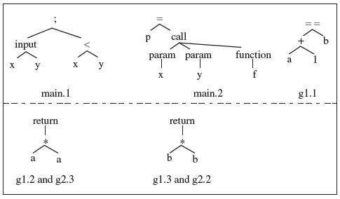
Example 9.7 Syntax trees for some nodes in Figure 9.5 are shown in Figure 9.6. Note the semicolon that labels the tree for node 1 in function main. It indicates left to right sequencing of statements or expressions.
Figure 9.6 Syntax trees for some nodes in the CFGs of functions main, g1, and g2 of Ρ shown in Figure 9.5. A semicolon (;) indicates left to right sequencing of two or more statements within a node.
Compare CFGs and select tests: In this step the CFGs for Ρ and P′ are compared and a subset of Τ selected. The comparison starts from the Start node of the main functions of Ρ and P′ and proceeds further down recursively identifying corresponding nodes that differ in Ρ and P′. Only tests that traverse such nodes are selected.
A test t is selected only if the execution traces in Ρ and P′differ, i.e., the traces traverse nodes n1 and n2 in the two CFGs that have different syntax trees.
While traversing the CFGs, two nodes n ϵ Ν and n′ ϵ N′ are considered equivalent if the corresponding syntax trees are identical. Two syntax trees are considered identical when their roots have the same labels and the same corresponding descendants (see Exercise 9.4). Function calls can be tricky. For example, if a leaf node is labeled as a function name foo, then the CFGs of the corresponding functions in Ρ and P′ must be compared to check for the equivalence of the syntax trees.
Example 9.8 Suppose that the basic blocks in nodes n and n′ in G and G′ have identical syntax trees shown in Figure 9.7(a). However, these two nodes are not considered equivalent because the CFGs of function foo in P, and foo′ in P′, are not identical. The difference in the two CFGs is due to different labels of edges going out of node 1 in the CFGs. In Figure 9.7(b), the edge labeled f goes to node 3 while the edge with the same label goes to node 2 in Figure 9.7(c).
Procedure for selecting modification traversing tests
|
Input: |
• G, G′ : CFGs of programs Ρ and P′ and syntax trees corresponding to each node in a CFG. • Test vector test(n) for each node n in each CFG. • T: Set of non-obsolete tests for P. |
|
Output: |
T′: A subset of Τ. |
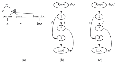
Figure 9.7 Syntax trees with identical function call nodes but different function CFGs. (a) Syntax tree for nodes n and n′, respectively, in G and G′. (b) CFG for foo in P. (c) CFG for foo′in P′.
/*
After initialization, procedure SelectTests is invoked. In turn SelectTests recursively traverses G and G′ starting from their corresponding start nodes. A node n in G found to differ from its corresponding node in G′ leads to the selection of all tests in Τ that traverse n.
*/
|
Step 1 |
Set T′ = Ø. Unmark all nodes in G and in its child CFGs. |
|
Step 2 |
Call procedure SelectTests(G.Start), G’.Start’), where G.Start and G’.Start are, respectively, the start nodes in G and G’. |
|
Step 3 |
T′ is the desired test set for regression testing P′. |
End of Procedure SelectTestsMain
Procedure: SelectTests (N, N′ )
|
Input: |
Ν, N′, where Ν is a node in G and Ν′ its corresponding node in G′. |
|
Output: |
T′. |
|
Step 1 |
Mark node Ν to ensure that it is ignored in the next encounter. |
|
Step 2 |
If Ν and Ν′ are not equivalent, then T′ = T′ ⋃ test(N) and return, otherwise go to the next step. |
|
Step 3 |
Let S be the set of successor nodes of N. Note that S is empty if Ν is the End node. |
|
Step 4 |
Repeat the next step for each nϵS. |
4.1 |
If n is marked then return else repeat the following steps. |
4.1.1 |
Let l =label(N ,n). The value of l could be t, f, or ϵ (for empty). |
4.1.2 |
n′ = getNode(l, Ν′ ). n′ is the node in G’ that corresponds to n in G. Also, the label on edge (Ν′, n′) is l. |
4.1.3 |
SelectTests(n, n′). |
|
Step 5 |
Return from SelectTests. |
End of Procedure SelectTests
Example 9.9 Next we illustrate the regression test selection procedure using Program P9.1. The CFGs of functions main, g1, and g2 are shown in Figure 9.5. test(n) for each node in the three functions is given in Example 9.6.
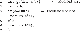
Now suppose that function g1 is modified by changing the condition at line 3 as shown in Program P9.2. The CFG of g1 changes only in that the syntax tree of the contents of node 1 is now different from that shown in Figure 9.5. We will use the SelectTests procedure to select regression tests for the modified program. Note that all tests in Τ in Example 9.5 are valid for the modified program and hence are candidates for selection.
Program P9.2
Let us follow the steps as described in SelectTestsMain. G and G’ refer to, respectively, the CFGs of Program P9.1 and its modified version–the only change being in g1.
SelectTestsMain.Step 1: T′ = Ø.
SelectTestsMain.Step 2: SelectTests (G.main.Start, G′ .main.Start).
SelectTests.Step 1: Ν = G.main.Start and N′ = G’.main.Start. Mark G.main.Start.
SelectTests.Step 2 G.main.Start and G’.main.Start are equivalent hence proceed to the next step.
SelectTests.Step 3 S = succ(G.Start) = {G.main.1}.
SelectTests.Step 4: Let n=G.main.1.
SelectTests.Step 4.1: n is unmarked, hence proceed further.
SelectTests.Step 4.1.1: l = label(G.main.Start, n) = ∊.
SelectTests.Step 4.1.2: n′ = getNode(∊, G’.main.Start)=G’.main.1.
SelectTests.Step 4.1.3: SelectTests(n, n′).
SelectTests.Step 1: N =G.main.1 and N′ =G’.main.1. Mark G.main.1.
SelectTests.Step 2 G.main.1 and G’.main.1 are equivalent hence proceed to the next step.
SelectTests.Step 3 S = succ(G.main.l) = {G.main.2, G.main.3}.
SelectTests.Step 4: Let n = G.main.2.
SelectTests.Step 4.1: n is unmarked hence proceed further.
SelectTests.Step 4.1.1: l = label(G.main.1, n) = t.
SelectTests.Step 4.1.2: n′ = getNode (l, G’.main.1)=G’.main.2.
SelectTests.Step 4.1.3: SelectTests(n, n′ ).
SelectTests.Step 1: N = G.main.2 and N′ = G’.main.2. Mark G.main.2.
As G.main.2 contains a call to g1, the equivalence needs to be checked with respect to the CFGs of g1 and g2. Ν and N′ are not equivalent due to the modification in gl. Hence T′ = tests(N) = tests(G.main.2) = {t1, t3}. This call to SelectTests terminates. We continue with the next element of S. Exercise 9.6 asks you to complete the steps in this example.
9.5.3 Handling function calls
The SelectTests algorithm compares respective syntax trees while checking for the equivalence of two nodes. In the event the nodes being checked contain a call to function f that has been modified to f′, a simple check as in Example 9.9 indicates non-equivalence if f and f′ differ along any one of the corresponding nodes in their respective CFGs. This might lead to selection of test cases that do not execute the code corresponding to a change in f.
Finding the equivalence of two corresponding nodes in the CFGs of Ρ and P′ requires careful attention to any function calls within the nodes.
Example 9.10 Suppose that g1 in Program P9.1 is changed by replacing line 4 by return (a*a*a). This corresponds to a change in node 2 in the CFG for g1 in Figure 9.5. It is easy to conclude that despite t1 not traversing node 2, SelectTests will include t1 in T′. Exercise 9.7 asks you to modify SelectTests, and the algorithm to check for node equivalence, to ensure that only tests that touch the modified nodes inside a function are included in T′.
9.5.4 Handling changes in declarations
The SelectTests algorithm selects modification traversing tests for regression testing. Suppose that a simple change is made to variable declaration and that this declaration occurs in the main function. SelectTests will be unable to account for the change made simply because we have not included declarations in the CFG.
One method to account for changes in declarations is to add a node corresponding to the declarations in the CFG of a function. This is done for the CFG of each function in P. Declarations for global variables belong to a node placed immediately following the Start node in the CFG for main.
A CFG might not capture changes in declarations. A simple way to tackle this problem is to have one node in the CFG for each declaration. Thus, a test will be selected if the corresponding trace traverses nodes containing declarations that differ. However, this method will likely lead to the selection of all tests as each will traverse a declaration node.
The addition of a node representing declarations will force SelectTests to compare the corresponding declaration nodes in the CFGs for Ρ and P′. Tests that traverse the declaration node will be included in T′ if the nodes are found not equivalent. The problem now is that any change in the declaration will force the inclusion of all tests from Τ in T′. This is obviously due to the fact that all tests traverse the node following the Start node in the CFG for main. Next we present another approach to test selection in the presence of changes in declarations.
Let declChangef be the set of all variables in function f whose declarations have changed in f′. Variables removed or added are not included in declChangef (see Exercise 9.8). Similarly, we denote by gdeclChange the set of all global variables in P whose declarations have changed.
Let usef(n) be the set of variable names used at node n in the CFG of function f. This set can be computed by traversing the CFG of each function and analyzing the syntax tree associated with each node. Any variable used–not assigned to–in an expression at node n in the CFG of function f is added to usef(n). Note that declChangef is empty when there has been no change in declarations of variables in f. Similarly, usef(n) is empty when node n in CFG(f) does not use any variable, e.g. in statement x = 0.
Procedure SelectTestsMainDecl is a modified version of procedure SelectTestsMain. It accounts for the possibility of changes in declarations and carefully selects only those tests that need to be run again for regression testing.
Procedure for selecting modification traversing tests while accounting for changes in variable declarations.
|
Input: |
|
|
Output: |
T′: A subset of Τ. |
Procedure: SelectTestsMainDecl
/*
Procedure SelectTestsDecl is invoked repeatedly after the initialization step. In turn SelectTestsDecl looks for any changes in declarations and selects those tests from Τ that traverse nodes affected by the changes. Procedure SelectTests, as decribed earlier, is called upon the termination of processDecl.
*/
|
Step 1 |
Set T′ = Ø. Unmark all nodes in G and in its child CFGs. |
|
Step 2 |
For each function f in G, call procedure SelectDeclTest f, declChangef , gdeclChange). Each call updates T′. |
|
Step 3 |
Call procedure SelectTest(G.Start, G’.Start’), where G.Start and G’.Start are, respectively, the start nodes in G and G’. This procedure may add new tests to T′. |
|
Step 4 |
T′is the desired test set for regression testing P'. |
End of Procedure SelectTestsMainDecl
Procedure: SelectTestsDecl (f, declChangef , gdeclChange)
|
Input: |
f is function name and declChangef is a set of variable names in f whose declarations have changed. 1 |
|
Output: |
T′. |
|
Step 1 |
Repeat the following step for each node n ϵ CFG(f). |
1.1 |
if use(n). ∩ declChangef ≠ Ø or use(n) ∩ gdeclChange ≠ Ø then T′= T′∪ test(n). |
End of Procedure SelectTestsDecl
The SelectTests procedure remains unchanged. Note that in the approach described above, the CFG of each function does not contain any nodes corresponding to declarations in the function. Declarations involving explicit variable initializations are treated in two parts: a pure declaration part followed by an initialization part. Initializations are included in a separate node placed immediately following the Start node. Thus any change in the initialization part of a variable declaration, such as “int x =0;” changed to “int x =1;” is processed by SelectTests.
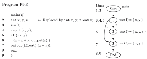
Example 9.11 Consider Program P9.3 and its CFG shown next to the code in Figure 9.8. As indicated, suppose that the type of variable z is changed from int to float. We refer to the original and the modified programs as Ρ and P′, respectively. It is easy to see that gdeclChange = Ø and declChangemain = {z}. Suppose the following test set is used for testing P.
Figure 9.8 Program and its CFG for Example 9.11.
We can easily trace CFG(P) for each test case to find the test vectors. These are listed below:
Abbreviating usemain as use, Step 1 in Procedure SelectTestsDecl proceeds as follows:
node 1: use(1)∩ declChangemain = Ø. Hence Τ′does not change,
node 2: use(2) ∩ declChangemain = {z}. Hence T′ = T′∪ test(2) = {t1, t3}.
node 3: use(3) ∩ declChangemain = Ø. Hence T′does not change.
Procedure SelectTestsDecl terminates at this point. Procedure SelectTests does not change T′as all the corresponding nodes in CFG(P) and CFG(P′) are equivalent. Hence we obtain the regression test T′= {t1 t3}.
9.6 Test Selection Using Dynamic Slicing
Selection of modification traversing tests using execution trace may lead to regression tests that are really not needed. Consider the following scenario. Program Ρ has been modified by changing the statement at line l. There are two tests t1 and t2 used for testing P. Suppose that both traverse l. The execution slice technique described earlier will select both t1 and t2.
Selection of regression tests using the execution trace method may lead to a larger than necessary test suite.
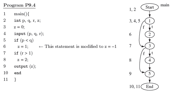
Figure 9.9 A program and its CFG for Example 9.12.
Now suppose that whereas t1 traverses l, the statement at l does not affect the output of Ρ along the path traversed from the Start to the End node in CFG(P). On the contrary, traversal of l by t2 does affect the output of P. In this case there is no need to test Ρ′on t1.
Example 9.12 Consider Program P9.4 that takes three inputs, computes, and outputs z. Suppose that Ρ is modified by changing the statement at line 6 as shown. Consider the following test set used for testing P:
Tests t1 and t3 traverse node 2 in CFG(P) shown in Figure 9.9, t2 does not. Hence if we were to use SelectTests described earlier, then T′ = {t1, t3}. This T′ is a set of modification traversing tests. However, it is easy to check that even though t1 traverses node 2, output z does not depend on the value of z computed at this node. Hence, there is no need to test P′ against t1 it needs to be tested only against t3.
We will now present a technique for test selection that makes use of program dependence graph and dynamic slicing to select regression tests. The main advantage of this technique over the technique based exclusively onthe execution slice is that it selects only those tests that are modification traversing and might affect the program output.
9.6.1 Dynamic slicing
Let Ρ be the program under test and t a test case against which Ρ has been executed. Let l be a location in Ρ where variable ν is used. The dynamic slice of Ρ with respect to t and ν is the set of statements in Ρ that lie in trace(t) and did effect the value of ν at l. Obviously, the dynamic slice is empty if location l was not traversed during this execution. The notion of a dynamic slice grew out of a static slice based on program Ρ and not on its execution.
Given a test t variable ν in program P, and an execution trace of Ρ with respect to t, a dynamic slice is the set of statements in the execution trace that did affect v.
Example 9.13 Consider Ρ to be Program P9.4 in Figure 9.9 and test t: < p = 1, q = 3, r = 2 >. The dynamic slice of Ρ with respect to variable z at line 9 and test t1 consists of statements at lines 4, 5, 7, and 8. The static slice of z at line 9 consists of statements at lines 3, 4, 5, 6, 7, and 8. It is generally the case that a dynamic slice for a variable is smaller than the corresponding static slice. For t: < p = 1, q = 0, r = 0 >, the dynamic slice contains 3, 4, 5, and 7. The static slice does not change.
9.6.2 Computation of dynamic slices
There are several algorithms for computing a dynamic slice. These vary across attributes such as the precision of the computed slice and the amount of computation and memory needed. A precise dynamic slice is one that contains exactly those statements that might affect the value of variable ν at the given location and for a given test input. We use DS(t,v,l) to denote the dynamic slice of variable ν at location l with respect to test t. When the variable and its location are easily identified from the context, we simply write DS to refer to the dynamic slice.
A precise dynamic slice consists of exactly the statements that affect a given variable ν at a given point in the program. Not all algorithms for computing a dynamic slice will always give a precise dynamic slice.
Next we present an algorithm for computing dynamic slices based on the dynamic dependence graph. Several other algorithms are cited in the bibliography section. GIven program P, test t, variable ν, and location l, computation of a dynamic slice proceeds in the following steps.
The dynamic dependence graph is used in computing the dynamic slice of Ρ with respect to a variable ν at a given location and test t.
Procedure: DSLICE
|
Step 1 |
Execute Ρ against test case t and obtain trace(t). |
|
Step 2 |
Construct the dynamic dependence graph G from Ρ and trace(t). |
|
Step 3 |
Identify in G the node n labeled l and containing the last assignment to v. If no such node exists then the dynamic slice is empty, otherwise proceed to the next step. |
|
Find in G the set DS(t, v, n) of all nodes reachable from n, including n. DS(t, v, n) is the dynamic slice of Ρ with respect to variable ν at location l for test t. |
End of Procedure DSLICE
In Step 2 of DSLICE we construct the dynamic dependence graph (DDG). This graph is similar to the program dependence graph (PDG) introduced in Chapter 1. Given program P, a PDG is constructed from Ρ whereas a DDG is constructed from the execution trace trace(t) of P. Thus, statements in Ρ that are not in trace(t) do not appear in the DDG.
While a program dependence graph is constructed from the given program, the dynamic program dependence graph is constructed from a trace of Ρ for a given test case.
Construction of G begins by initializing it with one node for each declaration. These nodes are independent of each other and no edge exists between them. Then a node corresponding to the first statement in trace(t) is added. This node is labeled with the line number of the executed statement. Subsequent statements in trace(t) are processed one by one. For each statement, a new node n is added to G. Control and data dependence edges from n are then added to the existing nodes in G. The next example illustrates the process.
Example 9.14 Consider the program in Figure 9.10. We have ignored the function header and declarations as these do not affect the computation of the dynamic slice in this example (see Exercise 9.11). Suppose now that 9.14 is executed against test case t :< x = 2, y = 4 >. Also, we assume that successive values of x are 0 and 5. Function f1(x) evaluates to 1, 2, and 3, respectively, for x = 2,0, and 5. Under these assumptions we get trace(t) = (1,21,31,4, 61,71,22,32,5 , 62,72,8); superscripts differentiate multiple occurrences of a node.
The construction of DDG is exhibited in Figure 9.10 above the solid line. To begin with, node labeled 1 is added to G. Node 2 is added next. This node is data independent on node 1 and hence an edge, indicated as a solid line, is added from node 2 to node 1.
Next, node 3 is added. This node is data dependent on node 1 as it uses variable x defined at node 1. Hence an edge is added from node 3 to node 1. Node 3 is also control dependent on node 2 and hence an edge, indicated as a dotted line, is added from node 3 to node 2. Node 4 is added next and data and control dependence edges are added, respectively, from node 4 to node 1 and to node 3. The process continues as described until the node corresponding to the last statement in the trace, i.e. at line 8, is added. The final DDG is shown in Figure 9.10 below the solid line.
Figure 9.10 A program and its dynamic dependence graph for Example 9.14 and test < x =2, y = 4 >. Function header and declarations omitted for simplicity. Construction process for the first four nodes is shown above the solid line.
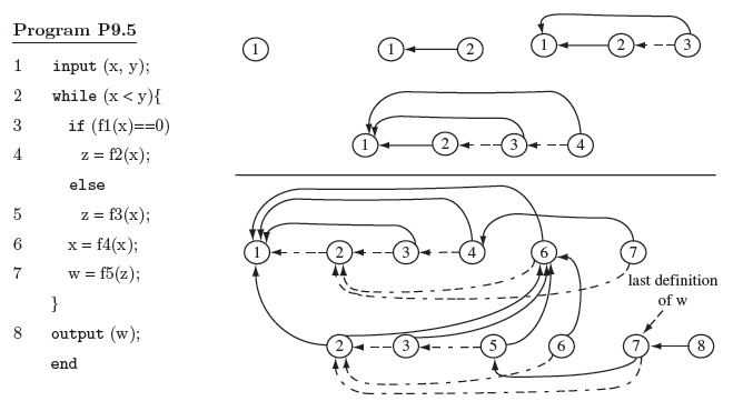
The DDG is used for the construction of a dynamic slice as mentioned in Steps 3 and 4 of procedure DSLICE. When computing the dynamic slice for the purpose of regression test selection, this slice is often based on one or more output variables which is w in Program P9.5.
The dynamic program dependence graph is used to obtain dynamic slices.
Example 9.15 To compute the dynamic slice for variable w at line 8, we identify the last definition of w in the DDG. This occurs at line 7 and, as marked in the figure, corresponds to the second occurrence of node 7 in Figure 9.10. We now trace backwards starting at node 7 and collect all reachable nodes to obtain the desired dynamic slice as {1, 2, 3, 5, 6, 7, 8} (also see Exercise 9.10).
9.6.3 Selecting tests
Given a test set Τ for P, we compute the dynamic slice of all, or a selected set of, output variables for each test case in T. Let DS(t) denote such a dynamic slice for t ϵ T. DS(t) is computed using the procedure described in the previous section. Let n be a node in Ρ modified to generate P′. Test t ϵ Τ is added to T′ if n belongs to DS(t).
Dynamic slices are computed for all or a selected subset of the output variables of a program.
We can use SelectTests to select regression tests but with a slightly modified interpretation of test(n). We now assume that test(n) is the set of tests t ϵ Τ such that n ϵ DS(t). Thus, for each node n in CFG(P), only those tests that traverse n and might have effected the value of at least one of the selected output variables are selected and added to T′.
Example 9.16 Suppose that line 4 in Program P9.5 is changed to obtain P'. Should t from Example 9.14 be included in Τ'? If we were to use only the execution slice, then t will be included in T′because it causes the traversal of node 4 in Figure 9.10. However, the traversal of node 4 does not effect the computation of w at node 8 and hence, when using the dynamic slice approach, t is not included in T′. Note that node 4 is not in DS(t) with respect to variable w at line 8 and hence t should not be included in T.
9.6.4 Potential dependence
The dynamic slice contains all statements in trace(t) that had an effect on program output. However, there might be a statement s in the trace that did not effect program output but may affect if changed. By not including s in the dynamic slice we exclude t from the regression tests. This implies that an error in the modified program due to a change in s might go detected.
A dynamic slice contains all statements in a program that had an impact on an output variable.
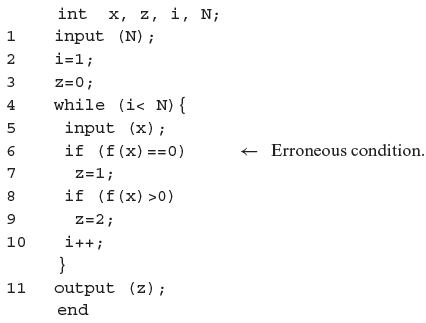
Example 9.17 Let Ρ denote Program P9.6. Suppose Ρ is executed against test case t: < Ν = 1, x = 1 > and that f(x) < 0 during the first and only iteration of the loop in P. We obtain trace(t) = (1,2,3,4,5,6,8,10,4,11). The DDG for this trace is shown in Figure 9.11; for this example ignore the edges marked as “p.” The dynamic slice DS(t, z, 11) = {3,11} for output z at location 11.
Program P9.6
Notice that DS(t, z, 11) does not include the node corresponding to line 6. Hence t will not be selected for regression testing of Ρ obtained by modifying the if statement at line 6. But, of course, t must be included in the regression test.
We define the concept of potential dependence to overcome the problem illustrated in the previous example. Let trace(t) be a trace of Ρ on test t. Let ν be a variable used at location Lν and P a predicate that appears at location Lp prior to the traversal of location Lν. A potential dependency is said to exist between ν and p when the following two conditions hold:
Potential dependance is used to include test cases that would otherwise be excluded when using the dynamic slicing algorithm mentioned earlier.
- ν is never defined on the subpath traversed from Lp to Lv but there exists another path, say r, from Lp to Lν where ν is defined.
- Changing the evaluation of p may cause path r to be executed.
The following example illustrates how to use the above definition to identify potential dependencies.
Example 9.18 Let us apply the above definition of potential dependence to Program P9.6 when executed against t as in Example 9.17. The subpath traversed from node 6 to node 11 contains nodes in the following sequence: 6, 8, 10, 4, 11. Node 11 has a potential dependency on node 6 because (i) z is never defined on this subpath but there exists a path r from node 6 to node 11 along which z is defined and (ii) changing the evaluation of the predicate at node 6 causes r to be executed. This potential dependency is shown in Figure 9.11. Note that one possible subpath r contains nodes in the following sequence: 6, 7, 8, 10, 4, 11.
Figure 9.11 Dynamic dependence graph for Program P9.6 obtained from trace(t), t: <N = 1, x = 1 >. Unmarked dotted edges indicate control dependence. Edges marked “p” indicate potential dependence.
Using a similar argument it is easy to show the existence of potential dependency between nodes 8 and 11. The two potential dependencies are shown by dotted edges labeled “p” in Figure 9.11.
Procedure to compute potential dependencies.
|
Input: |
• Program Ρ and its CFG G. There is exactly one node in G for each statement in P. • trace(t) for test t obtained by executing Ρ against t. • DDG(t). • Location L and variable ν in Ρ for which the potential dependencies are to be computed. |
|
Output: |
PD: Set of edges indicating potential dependencies between L and other nodes in DDG(t). |
Procedure: ComputePotentialDep
/*
Procedure ComputePotentialDep is invoked after the construction of the dynamic dependence graph G corresponding to a given trace. It uses G to determine reaching definitions of ν at location L. These definitions are then used to iteratively compute PD.
*/
For each program variable ν defined at location L, there exist a set of nodes known as the “reaching definition.” A node Lv is in this set if there is a path from the start of the CFG to Lv and then to node L without an intermediate redefinition of ν.
Static reaching definitions are computed from Ρ and not from its execution trace.
End of Procedure ComputePotentialDep
Example 9.19 Let us apply procedure ComputePotentialDep to compute potential dependencies for variable z at location 11 for trace(t) = (1,2,3,4,5,6,8,10,42,11) as in Example 9.17. The inputs to ComputePotentialDep include data from Program P9.6, G shown in Figure 9.11, trace(t), location L = 11, and variable ν = z.
Step 1: From Ρ we get the static reaching definitions of ν at L as S = {3,7,9}. Note that in general this is a difficult task for large programs and especially those that contain pointer references (see bibliographic notes for general algorithms for computing static reaching definitions).
Step 2: Node 3 has no control dependency. Noting from P, nodes 7 and 9 are control dependent on, respectively, nodes 6 and 8. Each of these nodes is in turn control dependent on node 4. Thus we get C = {4,6,8}.
Step 3: Node 3 contains the last definition of z in trace(t). Hence D = z.
Step 4: PD =Ø.
Step 5: Lv = 3. nodeSeq = (3,4,5,6,8,10,42,11). Each node in nodeSeq is marked NV. We show this as nodeSeq = (3NV,4NV, 5NV, 6NV, 7NV, 8NV, 10NV, 4NV,11NV)
Step 6: Select n = L = 11.
Step 6.1: n is marked NV hence we consider it.
Step 6.1.1: nodeSeq = (3NV,4NV, 5NV 6NV, 8NV, 10NV, 4NV, 11V). We have omitted the superscript 2 on the second occurrence of 4.
Step 6.1.2: As n is not in C, we ignore it and continue with the loop.
Step 6: Select n = L = 4.
Step 6.1: n is marked NV hence we consider it.
Step 6.1.1: nodeSeq = (3NV,4NV, 5NV 6NV, 8NV, 10NV, 4V, 11V).
Step 6.1.2: As n is in C, we process it. (a) PD = {4}. (b) Nodes 4 and 11 are not control dependent on any node and hence no other node needs to be marked.
Steps 6, 6.1, 6.1.1: Select n = 10. As n is marked NV we consider it and mark it V. nodeSeq = (3NV,4NV, 5NV 6NV, 8NV, 10V, 4V, 11V).
Step 6.1.2: Node 10 is not a control node hence we ignore it and move to the next iteration.
Steps 6, 6.1, 6.1.1: Select n = 8. This node is marked NV, hence we mark it V and process it. nodeSeq = (3NV,4NV, 5NV 6NV, 8V, 10V, 4V, 11V).
Step 6.1.2: Node 6 is in C hence (a) we add it to PD to get PD = {4, 8} and (b) mark node 4 as V because 8 is control dependent on these nodes. nodeSeq = (3NV,4NV, 5NV6V, 8V, 10V, 4V, 11V).
Steps 6, 6.1, 6.1.1: Select n = 6. This node is marked NV, hence we mark it V and process it. nodeSeq = (3NV,4NV, 5NV 6V, 8V, 10V, 4V, 11V).
Step 6.1.2: Node 8 is in C hence (a) we add it to PD to get PD = {4, 6, 8} and (b) there are no new nodes to be marked.
Steps 6, 6.1, 6.1.1, 6.1.2: Select n = 5. This node is marked NV, hence we mark it V and process it. nodeSeq = (3NV,4NV, 5V6V, 8V, 10V, 4V, 11V). We ignore 5 as it is not in C.
The remaining nodes in nodeSeq are either marked V or are not in C and hence will be ignored. The output of procedure ComputePotentialDep is PD = {4, 6, 8}.
Computing potential dependencies in the presence of pointers is a complex task. Several algorithms for computing such dependencies are available.
Computing potential dependences in the presence of pointers requires a complicated algorithm. See the bibliography section for references to algorithms for computing dependence relationships in C programs.
9.6.5 Computing the relevant slice
The relevant slice RS(t, v, n) with respect to variable ν at location n for a given test case t is the set of all nodes in the trace(t) which if modified may alter the program output. Given trace(t), the following steps are used to compute the relevant slice with respect to variable ν at location n.
A relevant slice of variable ν in program Ρ at location L and for a test input t is the set of all nodes in the program trace which if modified may alter the program output.
A relevant slice is derived from the dynamic program dependence graph by adding addition edges that correspond to potential dependence.
Example 9.20 Continuing with Example 9.19 and referring to Figure 9.11 that indicates the potential dependence, we obtain S = {1,4,5,6}, and hence RS(t, z,11) = S ⋃ DS(t, z,11) = {1,3,4,5,6,11}. If the relevant slice is used for test selection, test t in Example 9.17 will be selected if any statement on lines 1, 3, 4, 5, 6, and 11 is modified.
9.6.6 Addition and deletion of statements
Statement addition: Suppose that program Ρ is modified to P′ by adding statement s. Obviously, no relevant slice for Ρ would include the node corresponding to s. However, we do need to find tests in T, used for testing P, that must be included in the regression test set T′ for P′. To do so, suppose that (a) s defines variable x, as for example through an assignment statement, and (b) RS(t,x,l) is the relevant slice for variable x at location l corresponding to test case t ϵ T. We use the following steps to determine whether or not t needs to be included in T′.
Modification of a program via the addition on the deletion of statements may affect some relevant slices.
|
Step 1 |
Find the set s of statements s1,s2,…,sk,k≥ 0, that use x. Let nt, 1 ≤ i ≤ k denote the node corresponding to statement st in the DDG of P. A statement in S could be an assignment that uses x in an expression, an output statement, or a function or method call. Note that x could also be a global variable in which case all statements in Ρ that refer to x must be included in S. It is obvious that if k = 0 then the newly added statement s is useless and need not be tested. |
|
Step 2 |
For each test t ϵT, add t to T′ if for any j, 1 ≤j ≤ k, nj ϵ RS(t, x, l). |
Example 9.21 Suppose that Program P9.5 is modified by adding the statement x = g(w) immediately following line 4 as part of the then clause. The newly added statement will be executed when control arrives at line 3 and f1(x) = 0.
Set S of statements that use x is {2,3,4,5,6}. Now consider test t from Example 9.14. You may verify that the dynamic slice of t with respect to variable w at line 8 is the same as its relevant slice RS(8) which is {1,2,3,5,6,7,8} as computed in Example 9.15. Several statements in S belong to RS(t, w, 8) and hence t must be included in T′(also see Exercise 9.17).
Statement deletion: Now suppose that P′is obtained by deleting statement s from P. Let n be the node corresponding to s in the DDG of P. It is easy to see that all tests from Τ whose relevant slice includes n must be included in T′ .
Statement deletion and addition: An interesting case arises when Ρ′is obtained by replacing some statement s in Ρ by s′ such that the left side of s′ is different from that of s. Suppose that node n in the DDG of Ρ corresponds to s and that s′ modifies variable x. This case can be handled by assuming that s has been deleted and s′ added. Hence all tests t ϵ Τ satisfying the following conditions must be included in T′ (a) n ϵ RS(t, w, I) and (b) m ϵ RS(t,w,l) where node m in CFG(P) corresponds to some statement in Ρ that uses variable w.
Ρ′can be obtained by making several other types of changes in Ρ not discussed above. See Exercise 9.18 and work out how the relevant slice technique can be applied for modifications other than those discussed above.
9.6.7 Identifying variables for slicing
You might have noticed that we compute a relevant slice with respect to a variable at a location. In all examples so far, we used a variable that is part of an output statement. However, a dynamic slice can be constructed based on any program variable that is used at some location in P, the program that is being modified. For example, in Program 9.17 one may compute the dynamic slice with respect to variable z at line 9 or at line 10.
In large programs, the identification of variables and their locations could become an enormous task. Thus, one needs to carefully identify only the most critical variables and the locations where they are defined.
Some programs will have several locations and variables of interest at which to compute the dynamic slice. One might identify all such locations and variables, compute the slice of a variable at the corresponding location, and then take the union of all slices to create a combined dynamic slice (see Exercise 9.10). This approach is useful for regression testing of relatively small components.
In large programs there might be many locations that potentially qualify to serve as program outputs. The identification of all such locations might itself be an enormous task. In such situations a tester needs to identify critical locations that contain one or more variables of interest. Dynamic slices can then be built only on these variables. For example, in an access control application found in secure systems, such a location might be immediately following the code for processing an activation request. The state variable might be the variable of interest.
9.6.8 Reduced dynamic dependence graph
As described earlier, a dynamic dependence graph constructed from an execution trace has one node corresponding to each program statement in the trace. As the size of an execution trace is unbounded, so is that of the DDG. Here we describe another technique to construct a reduced dynamic dependence graph (RDDG). While an RDDG looses some information that exists in a DDG, the information loss does not impact the tests selected for regression testing (see Exercise 9.25). Furthermore, the technique for the construction of an RDDG does not require saving the complete trace in memory.
The size of a dynamic dependence graph is unbounded as it is directly proportional to that of the execution trace.
Construction of an RDDG, G proceeds during the execution of Ρ against a test t. For each executed statement s at location l, a new node n labeled l is added to G only when there does not already exist such a node. In case n is added to G, any of its control and data dependencies are also added. In case n is not added to G, the control and data dependences of n are updated. The number of nodes in the RDDG so constructed equals at most the number of distinct locations in P. In practice, however, most tests exercise only a portion of Ρ thus leading to a much smaller RDDG.
A reduced dynamic dependence graph contains at most one occurrence of each node in the program trace.
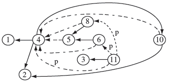
Example 9.22 Suppose 9.17 is executed against t and trace(t) = {1,2,3,41,5,6,8,9,10,| 42,52,62,82,102, | 43,53,63,7, 83,103, | 44,11}. Construction of RDDG G is shown in Figure 9.12. The vertical bars indicate the end of the first three iterations of the loop. Figure 9.12(a) shows the partial RDDG at the end of the first iteration of the loop, Figure 9.12(b) at the end of the second iteration, and Figure 9.12(c) the complete RDDG at the end of program execution. We have ignored the declaration node in this example.
Notice that none of the statements in trace(t) corresponds to more than one node in G. Also, note how new nodes and new dependence edges are added. For example, in the second iteration, a data dependence edge is added from node 4 to node 10, and from 10 to itself. The RDDG contains only 11 nodes in contrast to a DDG which would contain 22 nodes when constructed using the procedure described in Section 9.6.2.
The procedure for obtaining a dynamic slice from an RDDG remains the same as described in Section 9.6.2. To obtain the relevant slice one first discovers the potential dependences and then computes the relevant slice as illustrated in Section 9.6.5.
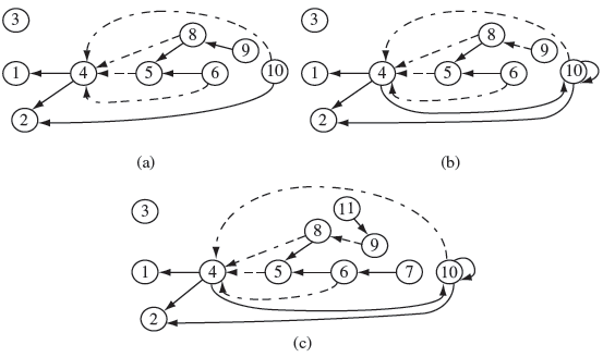
Figure 9.12 Reduced dynamic dependence graph for Program 9.17 obtained from trace(t) = {1,2,3,41, 5,6,8,9,10, | 42,52,62,82, 102, | 43,53,63,7,83, 103, | 44,11}. Intermediate status starting from (a) node 1 until node 10, (b) node 42 until node 102, and (c) complete RDDG for trace(t).
9.7 Scalability of Test Selection Algorithms
The execution slice and dynamic slicing techniques described above have several associated costs. First there is the cost of doing a complete static analysis of program Ρ that is modified to generate P′. While there exist several algorithms for static analysis to discover data and control dependencies, they are not always precise especially for languages that offer pointers. Second, there is the run time overhead associated with the instrumentation required for the generation of an execution trace. While this overhead might be tolerable for operating systems and non-embedded applications, it might not be for embedded applications.
The cost of dynamic slicing includes that of static program analysis and the construction of the dynamic dependence graph for every test input.
In dynamic slicing, there is the additional cost of constructing and saving the dynamic dependence graph for every test. Whether or not this cost can be tolerated depends on the size of the test suite and the program. For programs that run into several hundred thousands of lines of code and are tested using a test suite containing hundreds or thousands of tests, DDG (or the RDDG) at the level of data and control dependence at the statement level might not be cost effective at the level of system, or even integration, testing.
Thus, while both the execution trace and DDG-or RDDG-based techniques are likely to be cost effective when applied to regression testing of components of large systems, they might not be when testing the complete system. In such cases, one can use a coarse level data and control dependence analysis to generate dependence graphs. One may also use coarse level instrumentation for saving an execution trace. For example, instead of tracing each program statement, one could trace only the function calls. Also, dependence analysis could be done across functions and not across individual statements.
For very large programs, one might use coarse-level data and control dependence analysis to reduce the cost of generating dynamic dependence graphs.
Example 9.23 Consider Program P9.1 in Example 9.5. In that example we generate three execution traces using three tests. The traces are at the statement level.
Suppose that we want to collect the execution trace at the level of function calls. In this case the program needs to be instrumented only at call points, or only at the start of each function definition. Thus the total number of probes added to the program to obtain a function-level execution trace is equal to the number of functions in the program, three in this case–main, g1, and g2. The function traces corresponding to the three tests are shown in the following table:
t1
main, g1, main
t2
main, g2, main
t3
main, g1, main
Notice the savings in the number of entries in each execution trace. The function trace has a total of nine entries for all three tests whereas the statement level trace has 30. In general, the savings in storage requirements for a functional trace over statement trace will depend on the average size of the functions (see Exercise 9.35).
While tracing at a coarse level leads to reductions in the run time overhead, it also leads to a much smaller DDG. For example, rather than represent control and data dependencies across program variables, one can do the same across functions. In most practical applications, data and control dependencies at a coarse level will lead to smaller DDGs relative to those constructed using dependencies at the level of program variables.
In most applications, data and control dependence at a coarse-level will likely lead to smaller dynamic dependence graphs.
Consider two functions f1 and f2 in program P. Function f2 has data dependency on f1 if there is at least one variable defined in f1 such that its definition reaches f2. Similarly, f2 is control dependent on f1 when there are at least two paths from the start of Ρ to the end that pass through f1 but only one of these passes through f2 after having passed through f1 and the other path might be taken if a condition in f1 evaluated differently. It is important to note that construction of DDG (or RDDG) requires static analysis of Ρ to determine data and control dependence across various functions.
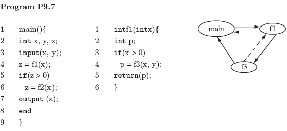
Figure 9.13 Dynamic data dependence graph for Program P9.7 corresponding to the function trace: main, f l, f 3, f l, and main.
Example 9.24 Program P9.7 consists of main and three functions f1, f2, and f3. Consider the function trace consisting of the following calling sequence: main, f1, f3, f1, and main. The DDG corresponding to this trace appears in Figure 9.13.
Notice the data and control dependence among various functions in the trace. main has data dependence on f1 due to its use of f1 to compute the value of z. Function f1 also has data dependence on main due to its use of x. f3 uses global variable y and hence has data dependence on main. Also, f3 is control dependent on f1 as it may or may not be called upon entry to f1 (see Exercise 9.22).
Computing dynamic slices using a DDG based on function traces can be tricky. First, one needs to ask the proper question. In the program variable based slicing discussed earlier, we are able to specify a variable and its location for slicing. Against what should the slice be constructed when traces are based on functions? Second, the DDG exhibits dependencies at the function level, and not at the level of program variables. Hence, how do we relate the slicing requirement to the DDG?
Computation of dynamic slices at the level of functions requires one to specify requirements for slices. This can be done by identifying variables of interest inside functions.
We can compute a dynamic slice based on a program variable at a specific location just as we did earlier. However, one needs to use static analysis to locate the function that contains the variable and its location. For example, if the slice is to be computed for z at line 7 in Program P9.7, then we know that this variable and location is inside main. Once the containing function has been identified, the dynamic slice is constructed using the DDG as before (see Exercise 9.23).
9.8 Test Minimization
Modification traversing test selection finds a subset T′of Τ to use for regression testing. Now suppose that Ρ contains n testable entities. Functions, basic block, conditions, and definition-use pairs are all examples of testable entities. Suppose that tests in Τ′cover, i.e. test, m < n of the testable entities. It is likely that there is an overlap among the entities covered by two tests in T′.
Test minimization is performed using one of more coverage criteria. These criteria could be black- or white-box.
We therefore ask: Is it possible, and beneficial, to reduce T′ to T'', such that T'' ⊆ T′ and each of the m entities covered by tests in T′ is also covered by tests in T''? Such a test reduction process is commonly referred in software testing as test minimization. Of course, we can also apply test minimization directly to Τ (see Exercise 9.28).
Example 9.25 Consider Program P9.7 and test set T={t1, t2, t3}. Figure 9.14 shows the CFG of P9.7. Let basic block be the entity of interest. The coverage of basic blocks for tests in Τ is as follows; note that we have excluded functions f2 and f3 from the coverage information assuming that these are library functions and that we do not have source code available to measure the corresponding block coverage.
t1 : main : 1, 2, 3 f1 : 1,3
t2 : main : 1,3 f1 : 1,3
t3 : main : 1,3 f1 : 1, 2, 3
Tests in Τ cover all six blocks, three in main and three in f1. However, it is easy to check that these six blocks can also be covered by t1 and t3. Hence rather than using T as a regression test one could also use T′= {t1,t3}, albeit with caution. Note that in this example the minimized test suite is unique.
A reduced (minimized) test suite might not have the same fault detection effectiveness as that of its container test set; however, the reduction in the effectiveness depends on the coverage criteria used. The stronger the coverage criterion, the less the reduction in the effectiveness.
One could obtain a significant reduction in the size of a test suite by applying coverage-based minimization as in the previous example. However, one might ask: Will the minimized test suite have the same fault detection effectiveness as the corresponding non-minimized version? The answer to this question depends on the modifications made to Ρ to obtain P′, the kind of faults in P′, and the entity used for minimization (see Exercise 9.29).
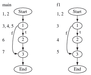
Figure 9.14 Control flow graph of Program P9.7.
9.8.1 The set cover problem
The test minimization problem can be formulated as the set cover problem. Let Ε be a set of entities and TE a set of subsets of E. A set cover is a collection of sets C ⊆ TE such that the union of all elements of ⊆ is TE. The set cover problem, more aptly the set cover optimization problem, is to find a minimal C. Relating this to test minimization, set Ε could be for example, a set of basic blocks, set TE a collection of sets of basic blocks covered by each test in Τ. The test minimization problem then is to find a minimal subset of TE that covers all elements of E.
The test minimization problem can formulated as a set cover problem.
Example 9.26 Let us formulate the test minimization problem as set cover problem with reference to Example 9.25. We get the following sets:
The solution to the test minimization problem is
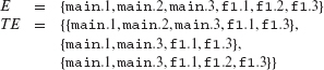
9.8.2 A procedure for test minimization
There exist several procedures for solving the set cover optimization problem. Given set TE, the naive algorithm computes the power set, 2TE, and selects from it the minimal covering subset. As the size of TE increases, the naive algorithm quickly becomes impractical (see Exercise 9.30).
The greedy algorithms or finding and minimizing a test set Τ selects test t that covers the maximal number of elements in P; an element might be a block, a decision, or any other entity depending on the minimization criterion.
The greedy algorithm is well known. Given a set of tests Τ and entities E, it begins by finding a test t ϵ Τ that covers the maximum number of entities in E. t is selected, removed from T, and the entities it covers are removed from E. The procedure now continues with the updated Τ and E. The greedy algorithm terminates when all entities have been covered. While the greedy algorithm is faster than the naive set enumeration algorithm, it fails to find the minimal set cover in certain cases. Below we present a slight variation of the greedy algorithm, named CMIMX.
The greedy algorithm might fail to find a minimal test set.
Procedure to find minimal covering set.
|
Input: |
An n × m matrix C. C(i, j) is 1 if test ti covers entity j, else it is 0. Each column of C contains at least one non-zero entry. Each column corresponds to a distinct entity and each row to a distinct test. |
|
Output: |
Minimal cover minCoν= {i1 ,i2,...., ik} such that for each column in C there is at least one non-zero entry in at least one row with index in minCov. |
Procedure: CMIMX
/* This procedure computes the minimal test cover for entities in C. */
|
Step 1 |
Set minCoν = Ø. yetToCover = m. |
|
Step 2 |
Unmark each of the n tests and m entities. An unmarked test is still under consideration, while a marked test is one already added to minCov. An unmarked entity is not covered by any test in minCov, whereas a marked entity is covered by at least one test in minCov. |
|
Step 3 |
Repeat the following steps while yetToCover > 0. |
3.1 |
Among the unmarked entities (columns) in C find those containing the least number of 1’s. Let LC be the set of indices of all such columns. Note that LC will be non-empty as every column in C contains at least one non-zero entry. |
3.2 |
Among all the unmarked tests (rows) in C that also cover entities in LC, find those that have the maximum number of non-zero entries. Let s be any one of these rows. |
3.3 |
Mark test s and add it to minCov. Mark all entities covered by test s. Reduce yetToCover by the number of entities covered by s. |
End of Procedure CMIMX
Example 9.27 Suppose program P has been executed against the five tests in test suite Τ. A total of six entities are covered by the tests as shown in the following table; 0 (1) in a column indicates that the corresponding entity is not covered (covered). The entities could be basic blocks in the program, functions, definition-uses, or any other testable element of interest. Further, a testable entity in Ρ not covered by any of the five tests is not included in the table.
Let us now follow procedure CMIMX to find the minimal cover set for the six entities. Input to the algorithm includes the 5 × 6 coverage matrix as shown in the above table.
Step 1: minCoν = Ø. yetToCover = 6.
Step 2: All five tests and six entities are unmarked.
Step 3: As yetToCover > 0, we execute the loop body.
Step 3.1: Among the unmarked entities, 4 and 6 each contain a single 1 and hence qualify as the highest priority entities. Thus LC={4,6}.
Step 3.2: Among the unmarked tests, t2 covers entities 1 and 4, and t4 covers entities 3 and 6. Both tests have identical benefits of 2 each in terms of the number of entities they cover. We arbitrarily select test t2. Thus s = 2.
Step 3.3: minCov = {2}. Test t2 is marked. Entities 1 and 4 covered by test t2 are also marked. yetToCover = 6 – 2 = 4.
Step 3.1: We continue with the second iteration of the loop as yetToCover > 0. Among the remaining unmarked entities, t6 is the one with the least cost (=1). Hence, LC = {6}.
Step 3.2: Only t4 covers entity 6 and hence s = 4.
Step 3.3: minCov = {2,4}. Test t4 and entities 3 and 6 are marked. yetToCover = 4 – 2 = 2.
Step 3.1: We continue with the third iteration of the loop as yetToCover > 0. The remaining entities, 2 and 5, have identical costs. Hence LC = {2,5}.
Step 3.2: Entities 2 and 5 are covered by unmarked tests t1, t3, and t5. Of these tests, t3 has the maximum benefit of 2. Hence s= 3.
Step 3.3: minCoν = {2,3,4}. Test t3 and entities 2 and 5 are marked. yetToCover =2 – 2 = 0.
Step 3: The loop and the procedure terminate with minCoν = {2,3,4} as the output.
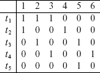
The difference between the greedy algorithm and CMIMX lies in Step 3.1 that is executed prior to applying the greedy test selection in Step 3.2. In this pre-greedy step, CMIMX prioritizes the entities for coverage. Entities covered by only one test get the highest priority, those covered by two tests get the next highest priority, and so on. One test that selects the highest priority entity is selected using the greedy algorithm. However, while the pre-greedy step allows CMIMX to find optimal solutions in cases where the greedy algorithm fails, it is not fail proof (see Exercises 9.31 and 9.32).
A modified version of the greedy algorithm prioritizes the entities to be covered and then applies the greedy algorithm.
9.9 Test Prioritization
Given programs Ρ and its modified version P′, the various techniques for test selection discussed so far lead to a regression test suite T′ derived from Τ used for testing P. While T′ is a subset of T, it might be overly large for testing P′. One might not have sufficient budget to execute P′ against all tests in T′. While test minimization algorithms could be used to further reduce the size of T′, this reduction is risky. Tests removed from T′ might be important for finding faults in P′. Hence one might not want to minimize T′. In such situations, one could apply techniques to prioritize tests in T' and then use only the top few high priority tests. In this section we introduce one technique for test prioritization.
Test prioritization aims at ranking tests in a test suite using some cost criterion. It is then up to a tester to decide how many tests to use for regression starting from the test at the top of the list.
Prioritization of tests requires a suitable cost criterion. Tests with lower costs are placed at the top of the list while those with higher cost at the bottom. The question obviously is: what cost criterion to use? Certainly, one could use multiple criteria to prioritize tests. It is important to keep in mind that tests being prioritized are the ones selected using some test selection technique. Thus, each test is expected to traverse at least some modified portion of P'. Of course, one could also prioritize all tests in Τ and then decide which ones to use when regression testing P'.
Test with lower cost are given high priority as compared to tests with higher cost. Of course, one could use multiple criteria to prioritize tests.
One cost criterion is derived directly from the notion of residual coverage. To understand residual coverage, suppose that Ε is a set of executable entities in P. For example, Ε could be any of set of basic blocks, definition-uses, all functions, or all methods in P. Suppose Ε is the set of all functions in P. Let E' ⊆ Ε be the set of functions actually called at least once during the execution of Ρ against tests in T'. We say that a function is covered if it is called at least once during some execution of P. Let us also assume that the library functions are excluded from Ε and hence from E'.
Residual coverage is one criterion used for prioritizing tests.
Let C(X) be the number of functions that remain to be covered after having executed Ρ against tests in set X ⊆ T'; initially C({}) =|E'|. C(X) is the residual coverage of Ρ with respect to X.
The cost of executing Ρ' against a test t in Τ' is the number of functions that remain uncovered after the execution of Ρ against t. Thus C(X) reduces, or remains unchanged, as tests are added to X. Hence the cost of a test is inversely proportional to the number of remaining functions it covers. Procedure PrTest, following the next example, computes the residual coverage for all tests in Τ' and determines the next highest priority test. This procedure is repeated until all tests in Τ' have been prioritized.
Example 9.28 Let Τ' = {t1, t2, t3} be the regression test for program Ρ' derived from test set Τ' for program P. Let E' be the set of functions covered when Ρ is executed against tests in Τ' and C({ }) = | E'| = 6. Now suppose t1 covers three of the six uncovered functions, t2 covers two, and t3 covers four. Note that there might be some overlap between the functions covered by the different tests.
The costs of t1, t2, and t3 are, respectively, 3, 4, and 2. Thus t3 is the lowest cost test and has the highest priority among the three tests. After having executed t3, we get C({t3}) = 2. We now need to select from the two remaining tests. Suppose that t1 covers none of the remaining functions and t2 covers 2. Then the cost of t1 is 2 and that of t2 is 0. Hence t2 has higher priority than t1. After executing t2, we get C({t2, t3}) = 0. The desired prioritized sequence of tests is < t3, t2, t1 >. Notice that execution of Ρ against t3 after having executed it against t3 and t1, will not reduce C(X) any further.
Procedure for prioritizing regression tests
|
Input: |
|
|
Output: |
PrT: A sequence of tests such that (a) each test in PrT belongs to T', (b) each test in Τ' appears exactly once in PrT, and (c) tests in PrT are arranged in the ascending order of cost. |
Procedure: PrTest
/*
PrT is initialized to test t with the least cost. The cost of each remaining test in Τ' is computed and the one with the least cost is appended to PrT and not considered any further. This procedure continues until all tests in Τ' have been considered.
*/
|
X' = Τ'. Find t ϵ X' such that |coν(t)| ≥ |coν(u)| for all u ϵ X', u ≠ t. |
|
|
Step 2 |
Set PrT =< t >, X' = X' {t}. Update entitiesCov by removing from it all entities covered by t. Thus entitiesCov = entitiesCoν cov(t). |
|
Step 3 |
Repeat the following steps while X' ≠ Ø and entityCoν ≠Ø. |
3.1 |
Compute the residual coverage for each test t ϵ Τ'. resCoν(t) = |entitiesCoν (coν(t) ∩ entitiesCoν)|. resCoν(t) indicates the count of currently uncovered entities that will remain uncovered after having executed Ρ against t. |
3.2 |
Find test t ϵ X' such that resCoν(t) ≤ resCoν(u), for all u ϵ X', u ≠ t. If two or more such tests exist then randomly select one. |
3.3 |
Update the prioritized sequence, set of tests remaining to be examined, and entities yet to be covered by tests in PrT. PrT = append(PrT, t), X' = X' {t}, and entitiesCoν = entitiesCoν coν(t). |
|
Step 4 |
Append to PrT any remaining tests in X'. All remaining tests have the same residual coverage which equals |entitiesCoν|. Hence these tests are tied. Random selection is one way to break the tie (also see Exercise 9.33). |
End of Procedure PrTest
Example 9.29 Consider application Ρ that consists of four classes C1, C2, C3, and C4. Each of these four classes is composed of one or more methods as follows: C1 = {m1, m12, m16}, C2 = {m2, m3, m4}, C3 = {m5, m6, m10, m11}, and C4 = {m7, m8, m9, m13, m14, m15}. In the following we refer to a method by an integer, e.g. m4, by 4.
Suppose that regression test set Τ' = {t1, t2, t3, t4, t5}. The methods covered by each test in Τ' are listed in the following table. Notice that method 9 has not been covered by any test in Τ' (see Exercise 9.26).
Let us now follow procedure PrTest to obtain a prioritized list of tests using residual coverage as the cost criterion. The inputs to PrTest are: Τ’, entitiesCov = {1,2,3,4,5,6, 7,8,10,11,12, 13,14,15,16}, and the test coverage vectors for each test in T' as in the table above. Note that we have excluded method 9 from entitiesCov as it is not covered by any test in Τ' and hence does not cause a difference in the relative residual coverage of each test.
Step 1:X' = {t1, t2, t4, t5}. t5 covers the largest number of functions–13– in X' and hence has the least cost.
Step 2:PrT = < t5 >. X' = {t1, t2, t3, t4}.
Step 3:We continue the process as X' and entityCoν are not empty.
Step 3.1:Compute the residual coverage for each test in X'.
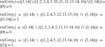
Step 3.2:t1 and t3 have the least cost. We arbitrarily select t3. One may instead use some other criteria to break the tie (see Exercise 9.33).
Step 3.3:PrT = < t5, t3 >. X' = {t1, t2, t4}, entitiesCoν = Ø.
Step 3: There is no function remaining to be covered. Hence we terminate the loop.
Step 4: t1, t2, and t4 remain to be prioritized. As entityCov is empty, the residual coverage criterion cannot be applied to differentiate among the priorities of these remaining tests. In this case we break the tie arbitrarily. This leads to PrT = < t5, t3, t1, t2, t4 >.
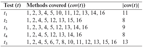
Test prioritization does not eliminate tests; it merely ranks them. It is then up to a tester to determine how many tests from the list to use for regression testing.
Prioritization of regression tests offers a tester an opportunity to decide how many and which tests to run under time constraints. Certainly, when all tests cannot be run, one needs to find some criteria to decide when to stop testing. This decision could depend on a variety of factors such as time constraint, test criticality, and customer requirements.
Note that the prioritization algorithm PrTest does not account for any sequencing requirements among tests in T'. As explained in Section 9.2.3, two or more tests in Τ' may be required to be executed in a sequence for P, and also for P'. Exercise 9.35 asks you to derive ways to modify PrTest to account for any test sequencing requirements.
Test prioritization must account for sequencing constraints amongst tests.
9.10 Tools
Regression testing for almost any non-trivial application requires the availability of a tool. The mere execution of large number of regression tests can be daunting and humanly impossible under the given time and budget constraints. Execution of tests may require application and test setup, recording of the outcome of each test, performance analysis, test abortion, and several others.
A variety of commercial tools perform exactly the tasks mentioned above, and a few others. However, there exist few tools that offer facilities for test selection using static and dynamic analysis, test minimization, and test prioritization. While test execution is an essential and time consuming task in regression testing, test selection, minimization, and prioritization, when used carefully, could lead to a significant reduction in the cost of regression testing.
There exist vela commercial and publicly available tools for regression testing. Few tools actually perform dynamic analysis or test prioritization.
Next we briefly review three advanced tools for regression testing that feature one or more of the techniques discussed in this chapter. The tools we have selected have all been developed in commercial environments and tested on large programs. This is by no means a complete set of tools; there exist several others developed in research and commercial environments that are not reviewed here.
Table 9.1 summarizes the capability of three tools across several attributes. Both ATAC/χSuds and TestTube work on a given source program written in C. Echelon is different in that it does test prioritization based on binary differencing technique. A key advantage of using binary differencing, in contrast to source code differencing, is that it avoids the complex static analyses required to determine the nature and impact of code changes such as variable renaming, or macro definitions.
The strength of ATAC/χSuds lies in the assessment of test adequacy across a variety of criteria as well as a seamless integration of regression testing with test execution, slicing, differencing, code coverage computation, test minimization across a variety of coverage criteria, test prioritization, a combination of minimization and prioritization, and test management. The strength of TestTube lies in its use of a coarse coverage criterion for test selection, namely function coverage.
None of the tools described here have reported an application in the embedded domain. It is important to note that due to the hardware storage and application timing constraints, a regression testing tool that is satisfactory in a non-embedded application might be unsuitable in an embedded environment.
Tool: Selenium
Link: http://seleniumhq.org/
Description
Table 9.1 A summary of three tools to aid in regression testing.
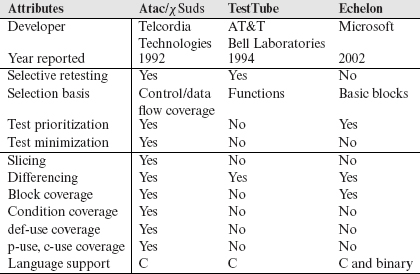
Selenium is fast becoming a popular tool for regression and system testing of Web applications. The Selenium IDE is a Firefox add-on that allows simple record and playback of interactions with the browser. The Selenium WebDriver allows for the automation of regression tests. The WebDriver enables driving a Web browser using its native support for automation. Support is available for Java, C#, Python, Ruby, Perl, and PHP. Several browsers including Firefox, Chrome, and Opera are also supported.
Tool: SilkTest
Link: http://www.borland.com/us/products/silk/index.aspx
Description
This tool is available from Borland. This tool is a part of the Silk tool suite that provides tools for test management, test automation, integration with an IDE such as Eclipse, and performance testing. SilkTest enables automating tests for WEb-based and other applications.
SUMMARY
Regression testing is an essential step in almost all commercial software development environments. The need for regression testing arises as corrective and progressive changes occur frequently in a development environment. Regression testing improves confidence in that existing and unchanged code will continue to behave as expected after the changes have been incorporated.
While test execution and logging of the test results are important aspects of regression testing, we have focused in this chapter on techniques for test selection, minimization, and prioritization. These three areas of regression testing require sophisticated tools and techniques. We have described in detail the most advanced techniques for test selection using dynamic slicing. These techniques evolved from research in program debugging and have found their way in regression testing.
While test selection using some form of program differencing is a safe technique for reducing the size of regression tests, test minimization is not. Despite research in the effect of test minimization on the fault detection effectiveness of the minimized test sets, discarding tests based exclusively on coverage is certainly risky and not recommended while testing highly critical systems. This is where test prioritization becomes useful. It simply prioritizes tests using one or more criteria and leaves to the tester the decision on which tests to select. Of course, one might argue that minimization assists the tester in that it takes such decision away from the tester. ATAC/χ Suds has a feature that allows a tester to combine minimization and prioritization and get the best of both worlds.
Exercises
9.1 In Example 9.2, we state “Under this assumption, when run as the first test, t3 will likely fail because the expected output will not match the output generated by SATM’. ” Under what conditions will this statement be false?
9.2 Given program Ρ and test t, explain the difference between an execution trace of Ρ against t when recorded as (a) a sequence of nodes traversed and (b) a set of nodes traversed. Use storage space as a parameter in your explanation. Give one example where a sequence is needed and a set representation will not suffice.
9.3 Draw the syntax trees in Example 9.7 not shown in Figure 9.6.
9.4 Write an algorithm that takes two syntax trees Tr and Tr' as inputs and returns true if they are identical and false otherwise. Recall from Section 9.5 that a leaf node might be a function name, say foo. In this case your algorithm must traverse the CFG of f, and the corresponding syntax trees, to determine equivalence.
9.5 In Example 9.9 there is only one function call at node 2 in main in Program P9.1. How will the application of SelectTests change if line 5 in main is replaced by: {p = g1(x, y) + g2(x, y)}?
9.6 Complete Example 9.9 to determine Τ' for the modified program.
9.7 Modify SelectTests such that Τ' includes only tests that traverse modified nodes in the main program and any called functions.
9.8 (a) Procedure SelectTestsMainDecl in Section 9.5.4 ignores the addition of any new variable declaration and deletion of any existing variable declaration. Does this imply that SelectTestsMainDecl is unsafe? (b) Suppose that variables added or removed from declarations in f are added to declChangef . In what ways will this change in the definition of declChange affect the behavior of SelectTestsMainDecl?
9.9 List at least one advantage of regression test selection using the dynamic slicing approach over the plain modification traversing approach.
9.10 Suppose that the output statement at line 8 in program P9.5 is replaced by: output (x, w);
Compute the dynamic slice with respect to x at line 8. Find the union of the dynamic slices computed with respect to variables x and w.
9.11 Consider test case t: < x =1, y = 0 >, Program P9.5, and its modification. Will t be selected by the SelectTests algorithm?
9.12 Consider the following test t, and the values of f1, f2, and f4, for program P9.5.
t: < x = 0, y = 3 > , f 1(0) = 0, f 2(0) = 4, f 4(0) = 5
Also assume that the output statement in Program P9.5 is as in Exercise 9.10. (a) Construct the DDG for Program P9.8 from its execution trace on t. (b) Compute the dynamic slices with respect to x and w at line 8. (c) Suppose Ρ' is P9.8 obtained from P9.5 by adding two initialization statements for w and z and removing the else part from the if statement.
Program P9.8
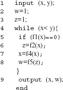
Will t be included in Τ' when using the dynamic slicing approach for test selection? (d) What property must be satisfied by a test case for it not to be included in Τ' when using the dynamic slicing approach? Construct one such test case, construct its DDG, and compute the dynamic slice with respect to w at line 9 in P9.8.
9.13 Consider Ρ to be Program P9.9.
Program P9.9
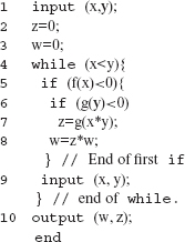
Suppose now that Ρ is executed against test t such that trace(t) = (1,2,3,4,5,6,8,9,4,10). (a) Construct the DDG for Ρ from trace(t). (b) Find the combined dynamic slice corresponding to variables w and z at line 10. (c) Compute the potential dependencies in the DDG. (d) Compute the combined relevant slice with respect to w and z.
9.14 Compute the relevant slice for program P9.6 corresponding to the trace obtained while executing it against t: < N = 2, x = 2, 4 >. Assume that f(2) = 0 and f(4) > 0.
9.15 Let Ρ and P' be the original and the modified programs, respectively. Let Τ be the tests for P. Suppose that P' is obtained by modifying an output statement s in P. Suppose also that s is the last executable statement in P. Which tests in Τ will not be selected when using the execution slice approach? The dynamic slicing approach?
9.16 Refer to Examples 9.17 and 9.20 and let Ρ be Program P9.6. Let e denote some error in Ρ that is corrected to create P'. Assume that correction of e requires a change to one of the existing statements, or the addition/deletion of a statement. You may also change the specification so that Ρ becomes erroneous. Now suppose that Ρ is executed against test t and e is not detected. Construct an e that will go undetected if (a) DS(t, z, 11) and (b) RS(t, z, 11) are used for test selection.
9.17 Consider the modification of Program P9.5, as indicated in Example 9.21. Suppose that t: < x = 1, y = 0 > and t ϵ T. Will t be selected for inclusion in Τ' by steps given in Section 9.6.6?
9.18 (a) Suppose that Program P9.9 is modified by removing a predicate as shown in Program P9.10. Should test t from Exercise 9.13 be included in the regression test for Program P9.10? (b) Now suppose that Program P9.10 is Ρ and is modified to Program P9.9 by adding predicate g(y) < 0. Consider test t such that trace(t) = {1,2,3,4,5,6,7,8,4,9}. Should t be included in the regression test for Program P9.9? (c) Give a general condition that can be used to decide whether or not a test should be included in T' when a predicate is added.
Program P9.10
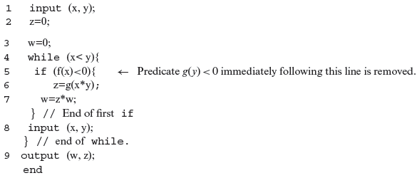
9.19 Let Ρ be a program tested against test set T. Under one maintenance scenario, P' is derived from Ρ through a series of modifications. These modifications are a mix of statement addition and deletion, predicate addition and deletion, addition of and removal of output variables, and perhaps others. Propose a systematic way of applying the relevant slice-based test selection technique that is scalable to large programs under the above maintenance scenario.
9.20 Dynamic slicing was originally proposed as a technique to aid in debugging programs. Subsequently it found an application in regression test selection. While the technique remains unchanged regardless of its application, the program dependence graph used as a source for computing the dynamic or relevant slice can be simplified when used for regression testing. Explain why.
9.21 Explain how one could use dynamic slicing as an aid in (i) program understanding and (ii) locating code corresponding to a specific feature implemented in a program.
9.22 Consider Program P9.7 in Figure 9.13. Suppose the following function trace trace(t) is obtained by executing the program against test t: main, f1, f2, main. (a) Draw the dynamic dependence graph from trace(t). (b) Now suppose a change is made in function f3. Will t be included in the regression test? (c) Will t be included in the regression test if a change is made to f1?
9.23 Compute the dynamic slice from the DDG in Figure 9.13 with respect to variable z at line 7.
9.24 Explain how you would compute potential dependencies in a DDG constructed out of function traces.
9.25 Exactly one node for each statement in the execution trace of Ρ appears in an RDDG constructed using the procedure described in Section 9.6.8. While such an RDDG is useful for regression test selection, it looses some information needed for constructing the dynamic slice with respect to a variable when debugging P. What information is lost and how does the loss might affect debugging of Ρ?
9.26 In Example 9.29, method 9 is not covered by any test in the regression test suite T'. Noting that Τ' ⊆ T, and Τ is the test set for application P, what might be the possible explanations for the lack of coverage of method 9 by tests in Τ'?
9.27 In what ways does a call graph differ from the dynamic dependence graph based on function trace?
9.28 Let T be a set of non-obsolete tests for P. Let P' be obtained by modifying P. Regression testing of P' is done using a subset Τ' of tests in Τ. What is the advantage of applying coverage-based test minimization procedure as in Section 9.8 to (a) Τ' and (b) T?
9.29 Let T be a test suite for testing Ρ and Τ' a minimized test suite for testing the modified version P' of P. Give reasons why the fault detection effectiveness of Τ' might be less than that of Τ. Construct an example to show that indeed there exist cases where a fault in P' is detected by a test case in Τ but by none in T'.
9.30 What is the time complexity of the naive algorithm for finding the minimal test set? Suppose that program Ρ is tested against n tests and a total of m entities are covered. Estimate how long it will take to find the minimal covering set when n = 100, m = 300; make suitable assumptions about the time it takes to perform various operations, e.g. set enumeration, required by the naive algorithm.
9.31 Consider the following “tricky” set cover problem. Let E = {1,2, … ,p} where P = 2k+1 – 2 for some k > 0. Let TE = {S1,S2,...,Sk,X, Y}, be such that (a) Si and Sj are disjoint for all 1 ≤ (i, j)≤ k,i≠ j, (b) Si contains 2i elements, (c) S1∪S2 ∪...∪Sk = E, and (d) X contains half the elements from each Si and Y contains the remaining half. Thus X ∩ Y = Ø and X ∪Y = E. The problem is to find the minimal set cover of E.
For example, for k = 2 we have E = {1,2,3,4,5,6}, TE = {S1, S2, X, Y}, S1 = {1,2},S2 = {3,4,5,6}, X = {1,3,4}, and Y = {2,5,6}. The minimal cover for this problem is {X, Y}. Show that both the greedy and the CMIMX algorithms fail to compute the minimal cover.
9.32 What is the importance of Step 3.1 in algorithm CMIMX?
9.33 In Example 9.29, two tests in Step 1 may tie for the minimum cost. A tie could also occur in Step 4 in procedure PrTest. Suggest at least two quantitative criteria that could be used to break the tie instead of breaking it through random selection as mentioned in procedure PrTest.
9.34 Let Τ' be a regression test for program P'. Let X = {<T'1>,<T'2>, .... , < T'k >}, k > 0 be a set of sequences of tests such that each sequence <T'i> contains tests from Τ' and that each test in Τ' occurs in at least one sequence in X. Modify PrTest to account for the requirement that if any < T'i > is selected for execution, the given sequencing constraint is not violated. Note that the sequences in X might not be disjoint.
9.35 Given a program Ρ composed of n functions and m tests, develop a formula to estimate the savings in storage requirements for function-level over statement-level execution traces. Make assumptions about the function size and coverage with respect to each test. How will your formula change for object-oriented programs where function-level execution trace is replaced by method-level execution trace?