2

Preliminaries: Mathematical

The purpose of this introductory chapter is to familiarize the reader with the basic mathematical concepts related to software testing. These concepts will likely be useful in understanding the material in subsequent chapters.

2.1  Predicates and Boolean Expressions

Let relop denote a relational operator in the set {<, >, ≤, ≥, =, ≠}. Let bop denote a Boolean operator in the set {∧, ∨, , ¬} where ∧, ∨, and are binary Boolean operators and ¬ is a unary Boolean operator. A Boolean variable takes on values from the set {true, false}. Given a Boolean variable a, ¬a and denote the complement of a.

 

A relational expression is an expression of the form e₁ relop e₂ where e₁ and e₂ are expressions that assume values from a finite or infinite set S. It should be possible to order the elements of S so that e₁ and e₂ can be compared using any one of the relational operators.

A predicate is a Boolean function that evaluates to true or false. It consists of relational symbols such as “<” and “>”, and Boolean connectors such as “and” and “or”. In computer programs such a function is also known as condition. A condition can be represented as a simple predicate or a compound predicate. A simple predicate is a Boolean variable or a relational expression where any one or more variables might be negated. A compound predicate is a simple predicate or an expression formed by joining two or more simple predicates, possibly negated, with a binary Boolean operator. Parentheses in any predicate indicate groupings of variables and relational expressions. Examples of predicates and other terms defined in this section are given in Table 2.1.

 

Table 2.1 Examples of terms defined in Section 2.1.

Item	Examples	Comment
Simple predicate	p q ∧ r a + b < c	p, q, and r are Boolean variables; a, b, and c are integer variables.
Compound predicate	¬(a + b < c) (a + b < c) ∧ (¬p)	Parentheses are used to make explicit the grouping of simple predicates.
Boolean expression	p, ¬p p ∧ q ∨ r
Singular Boolean expression	p ∧ q ∨ ∧ s	p, q, r, and s are Boolean variables.
Non-singular Boolean expression	p ∧ q ∨ ∧ p

A Boolean expression is composed of one or more Boolean variables joined by Boolean operators. In other words, a Boolean expression is a predicate that does not contain any relational expression. When it is clear from the context, we omit the ∧ operator and use the + sign instead of ∨. For example, Boolean expression p ∧ q ∨ ∧ s can be written as pq + s.

Note that the term pq is also known as a product of variables p and q. Similarly, the term rs is the product of Boolean variables r and s. The expression pq + s is a sum of two product terms pq and s. We assume left-to-right associativity for operators. Also, and takes precedence over or.

Each occurrence of a Boolean variable, or its negation, inside a Boolean expression, is considered as literal. For example, p, q, r, and p are four literals in the expression p ∧ q ∨ ∧ p.

A predicate p_r can be converted to a Boolean expression by replacing each relational expression in p_r by a distinct Boolean variable. For example, the predicate (a + b < c) ∧ (¬d) is equivalent to the Boolean expression e₁ ∧ e₂ where e₁ = a + b < c and e₂ = ¬d.

A Boolean expression is considered singular if each variable in the expression occurs exactly once. Consider the following Boolean expression Ε that contains k distinct Boolean expressions e₁, e₂, . . . , e_k.

 

 

For 1 ≤ i ≤ k, 1 ≤ j ≤ k, i ≠ j, we say that e_i and e_j are mutually singular if they do not share any variable. e_i is considered a singular component of Ε if and only if e_i is singular and is mutually singular with each of the other k – 1 components of E. e_i is considered non-singular if and only if it is non-singular by itself and is mutually singular with the remaining k – 1 elements of E.

 

A Boolean expression is considered to be in disjunctive normal form when it is expressed as a sum of product terms. It is in conjunctive normal form when expressed as a product of sums of terms. For example, pq + s is a DNF expression. A Boolean expression is in conjunctive normal form, also referred to as CNF, if it is written as a product of sums. For example, the expression (p + )(p + s)(q + )(q + s), is a CNF equivalent of expression pq + s. Note that any Boolean expression in CNF can be converted to an equivalent DNF and vice versa.

 

A Boolean expression can also be represented as an abstract syntax tree as shown in Figure 2.1. We use the term AST(p_r) for the abstract syntax tree of a predicate p_r. Each leaf node of AST(p_r) represents a Boolean variable or a relational expression. An internal node of AST(p_r) is a Boolean operator such as ∧, ∨, , and ¬, and is known as an AND node, OR node, XOR node, and a NOT node, respectively.

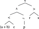
Figure 2.1 An abstract syntax tree for compound predicate (a + b < c) ∧ (¬p) ∨ (r > s).

2.2  Control Flow Graph

A control flow graph (CFG) captures the flow of control in a program. It consists of basic bocks and directed arcs connecting the blocks. Such a graph assists testers in the analysis of a program to understand its behavior in terms of the flow of control. A control flow graph can be constructed manually without much difficulty for relatively small programs, say containing less than about 50 statements. However, as the size of the program grows, so does the difficulty of constructing its control flow graph and hence arises the need for tools.

 

A CFG is also known by the names flow graph or program graph. However, it is not to be confused with the program dependence graph introduced in Section 2.5. In this section, we explain what a control flow graph is and how to construct one for a given program.

2.2.1  Basic blocks

Let P denote a program written in a procedural programming language, be it high level as C or Java, or a low level such as the 80 × 86 assembly. A basic block is the longest possible sequence of consecutive statements in a program such that control can enter the block only at the first statement and exit from the last. Thus, there cannot be any conditional statement inside a basic block other than at its end. Thus, a block has unique entry and exit points. These points are the first and the last statements, respectively, within a basic block. Control always enters a basic block at its entry point and exits from its exit point. There is no possibility of exit or a halt at any point inside the basic block except at its exit point. The entry and exit points of a basic block coincide when the block contains only one statement.

 

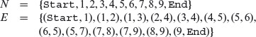
Example 2.1   The following program takes two integers x and y and outputs x^y. There are a total of 17 lines in this program including the begin and end. The execution of this program begins at line 1 and moves through lines 2, 3, and 4 to line 5 containing an if statement. Considering that there is a decision at line 5, control could go to one of two possible destinations at line 6 and line 8. Thus, the sequence of statements starting at line 1 and ending at line 5 constitutes a basic block. Its only entry point is at line 1 and the only exit point is at line 5.

Program P2.1

1  begin

2      int x, y, power;

3      float z;

4      input (x, y);

5      if (y<0)

6        power = -y;

7      else

8        power = y;

9      z = 1;

10      while (power! = 0){

11         z = z∗x;

12         power = power -1;

13      }

14      if (y<0)

15        z = 1/z;

16      output (z);

17   end

 

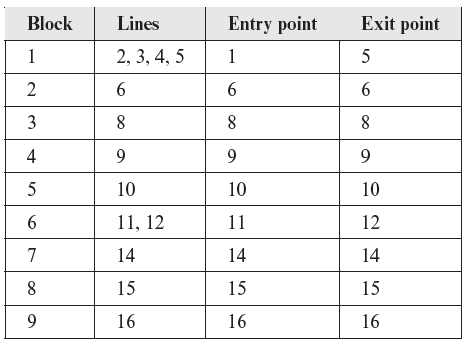
A list of all basic blocks in P2.1 is given below.

P2.1 contains a total of 9 basic blocks numbered sequentially from 1 to 9.

Note how the while at line 10 forms a block of its own. Also note that we have ignored lines 7 and 13 from the listing because these are syntactic markers, and so are begin and end that are also ignored.

Note that some tools for program analyses place a procedure call statement in a separate basic block. If we were to do that then we will place the input and output statements in P2.1 in two separate basic blocks. Consider the following sequence of statements extracted from P2.1.

 

1   begin

2     int x, y, power;

3     float z;

4     input (x, y);

5     if (y<0)

 

In the previous example, lines 1 through 5 constitute one basic block. The above sequence contains a call to the input function. If function calls are treated differently, then the above sequence of statements contains three basic blocks, one comprising lines 1 through 3, the second comprising line 4, and the third comprising line 5.

Function calls are often treated as blocks of their own because they cause the control to be transferred away from the currently executing function and hence raise the possibility of abnormal termination of the program. In the context of flow graphs, unless stated otherwise, we treat calls to functions like any other sequential statement that is executed without the possibility of termination.

2.2.2  Flow graphs

A flow graph G is defined as a finite set Ν of nodes and a finite set Ε of directed edges. A flow graph is another name for a CFG. It consists of nodes and directed edges. Each node represents a basic block in the program and each edge represents the flow of control from its source node to the destination node. An edge (i, j) in E, with an arrow directed from i to j, connects nodes n_i and n_j in N. We often write G = (Ν, E) to denote a flow graph G with nodes in Ν and edges in E. Start and End are two special nodes in Ν and are known as distinguished nodes. Every other node in G is reachable from Start. Also, every node in Ν has a path terminating at End. Node Start has no incoming edge and node End has no outgoing edge.

 

In a flow graph of program P, we often use a basic block as a node and edges indicate the flow of control across basic blocks. We label the blocks and the nodes such that block b_i corresponds to node n_i . An edge (i, j) connecting basic blocks b_i and b_j implies that control can go from block b_i to block b_j. Sometimes we will use a flow graph with one node corresponding to each statement in P.

A pictorial representation of a flow graph is often used in the analysis of the control behavior of a program. Each node is represented by a symbol, usually an oval or a rectangular box. These boxes are labeled by their corresponding block numbers. The boxes are connected by lines representing edges. Arrows are used to indicate the direction of flow. A block that ends in a decision has two edges going out of it. These edges are labeled true and false to indicate the path taken when the condition evaluates to true and false, respectively.

 

Example 2.2   The flow graph for P2.1 is defined as follows:

Figure 2.2(a) depicts this flow graph. Block numbers are placed right next to or above the corresponding box. As shown in Figure 2.2(b), the contents of a block may be omitted, and nodes are represented by circles, if we are interested only in the flow of control across program blocks and not their contents.

Figure 2.2 Flow graph representations of Program P2.1. (a) Statements in each block are shown. (b) Statements within a block are omitted.

2.2.3  Paths

Consider a flow graph G = (N, E). A sequence of k edges, k > 0, (e₁, e₂, . . . , e_k), denotes a path of length k through the flow graph if the following sequence condition holds: Given that n_p, n_q, n_r, and n_s are nodes belonging to N, and 0 < i < k, if e_i = (n_p, n_q) and e_i+1 = (n_r, n_s) then n_q = n_r.

 

Thus, for example, the sequence ((1, 3), (3, 4), (4, 5)) is a path in the flow graph shown in Figure 2.2. A path through a flow graph is a sequence of edges. It indicates the flow of control in the corresponding program. Not all paths extracted from a flow graph might be feasible implying that there does not exist any test input that will exercise an infeasible path in the corresponding program. However, ((1, 3), (3, 5), (6, 8)) is not a valid path through this flow graph. For brevity, we indicate a path as a sequence of blocks. For example, in Figure 2.2, the edge sequence ((1, 3), (3, 4), (4, 5)) is the same as the block sequence (1, 3, 4, 5).

For nodes n, m ∈ N, m is said to be a descendent of n if there is a path from n to m; in this case, n is an ancestor of m and m its descendent. If, in addition, n ≠ m, then n is a proper ancestor of m, and m a proper descendent of n. If there is an edge (n, m) ∈ E, then m is an immediate successor of n and n the immediate predecessor of m.

The set of all nodes that can be reached from node n along a path of length one or more is known as the successor set of node n. Similarly, the set of all nodes from which there exists a path of length one or more to node n is known as the predecessor set for node n. The set of successor and predecessor nodes of n is denoted as succ(n) and pred(n), respectively. The Start node has no ancestor and the End node has no descendent.

A path through a flow graph is considered complete if the first node along the path is Start and the terminating node is End. A path p through a flow graph for program P is considered feasible if there exists at least one test case that when input to P causes p to be traversed. If no such test case exists, then p is considered infeasible. Whether or not a given path is feasible is an undecidable problem. This statement implies that it is not possible to write an algorithm that takes as inputs an arbitrary program and a path through that program, and correctly outputs whether or not this path is feasible for the given program.

A subsequence of a path is subpath. A subpath that starts with the start node is known as an initial subpath. Given paths p = {n₁, n₂, . . . , n_t} and s = {i₁, i₂, . . . , i_u}, s is a subpath of p if for some 1 ≤ j ≤ t and j + u – 1 ≤ t, i₁ = n_j, i₂ = n_j+1, . . . , i_u = n_j+u–1. In this case, we also say that s and each node i_k for 1 ≤ k ≤ u, are included in p. Edge (n_m, n_m+1) that connects nodes n_m and n_m+1, is considered included in p for 1 ≤ m ≤ (t – 1).

Each path or subpath p in a CFG can be represented by a path vector of length e = |E|. A path vector is a list of n 0’s and 1’s. Each entry on the list corresponds to an edge in the flow graph. A 0 entry indicates that the corresponding edge does not lie along that path while a 1 indicates it does. Each entry in a path vector corresponds to an edge in the CFG and indicates the number of times that edge has been traversed along the path. Note that a path vector for a subpath will have 0’s corresponding to the edges not included in that subpath. We shall denote a path vector as V_p.

 

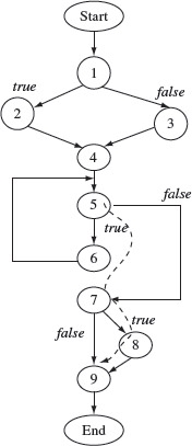
Example 2.3   In Figure 2.2, the following two are complete and feasible paths of lengths 10 and 9, respectively. The paths are listed using block numbers, the start node, and the terminating node.

Figure 2.3 shows the first of these two complete paths:

p₁ = (Start, 1, 2, 4, 5, 6, 5, 7, 8, 9, End)

p₂ = (Start, 1, 3, 4, 5, 6, 5, 7, 9, End)

As there are 13 edges in Figure 2.2(b), the path vector consists of 13 entries, one corresponding to each edge in the set Ε in Example 2.2. Assuming that the first entry in the path vector corresponds to the first entry in E, the second to the second entry in E, and so on, we obtain the following path vectors for p₁ and p₂.

V_p1 = [1101011111011]

V_p1 = [1010111110101]

(4, 5, 6) is a subpath of p₁. (Start, 1, 2, 4, 5) is an initial subpath. The next two paths of lengths 3 and 4 are incomplete. The first of these two paths is shown by a dashed line in Figure 2.3.

Figure 2.3 Flow graph representation of Program P2.1. A complete path is shown using bold edges and a sub-path using a dashed line.

p₃ = (5, 7, 8, 9)

p₄ = (6, 5, 7, 9, End)

The next two paths of lengths 10 and 7 are complete but infeasible.

p₅ = (Start, 1, 3, 4, 5, 6, 5, 7, 8, 9, End)

p₆ = (Start, 1, 2, 4, 5, 7, 9, End)

Finally, the next two paths are invalid as they do not satisfy the sequence condition stated earlier.

p₇ = (Start, 1, 2, 4, 8, 9, End)

p₈ = (Start, 1, 2, 4, 7, 9, End)

Nodes 2 and 3 in Figure 2.3 are successors of node 1, nodes 6 and 7 are successors of node 5, and nodes 8 and 9 are successors of node 7. Nodes 6, 7, 8, 9, and End are descendents of node 5. We also have succ(5)= {5, 6, 7, 8, 9, End} and pred(5)={Start, 1, 2, 3, 4, 5, 6}. Note that in the presence of loops, a node can be its own ancestor or descendent.

There can be many distinct paths through a program. Each additional condition in a program adds at least one path. A program with no condition contains exactly one path that begins at node Start and terminates at node End. However, each additional condition in the program increases the number of distinct paths by at least one. Depending on their location, conditions can have an exponential effect on the number of paths.

 

Example 2.4   Consider a program that contains the following statement sequence with exactly one statement containing a condition. This program has two distinct paths: one that is traversed when C₁ is true and the other when the condition is false.

begin

S₁;

S₂;

.

.

.

if (C₁) {. . .}

.

.

.

S_n;

end

 

We modify the program given above by adding another if. The modified program, shown below, has exactly four paths that correspond to four distinct combinations of conditions C₁ and C₂.

 

begin

S₁;

S₂;

.

.

.

if (C₁) {. . .}

.

.

.

if (C₂) {. . .}

S_n;

end

 

Notice the exponential effect of adding an if on the number of paths. However, if a new condition is added within the scope of an if statement then the number of distinct paths increases only by 1 as is the case in the following program that has only three distinct paths.

 

begin

S₁;

S₂;

 .

 .

 .

  if (C₁) {

 .

 .

 .

  if (C₂) {. . .}

 .

 .

 .

}

.

.

.

S_n;

end

 

The presence of loops can enormously increase the number of paths. Loops can significantly increase the number of paths in a program making exhaustive testing nearly impossible. Some assumptions on the distribution of the inputs can be used to estimate the number of paths in a program in the presence of loops and thus derive a few tests to test loops. Each traversal of the loop body adds a condition to the program thereby increasing the number of paths by at least one. Sometimes the number of times a loop is to be executed depends on the input data and cannot be determined prior to program execution. This becomes another cause of difficulty in determining the number of paths in a program. Of course, one can compute an upper limit on the number of paths based on some assumption on the input data.

 

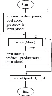
Example 2.5   Program P2.2 inputs a sequence of integers and computes their product. A Boolean variable done controls the number of integers to be multiplied. A flow graph for this program appears in Figure 2.4.

Program P2.2

1   begin

2   int num, product;

3   bool done;

4   product=1;

5   input(done);

6   while (!done) {

7       input(num);

8   product=product*num;

9       input(done);

10  }

11  output(product);

12  end

Figure 2.4 Flow graph of Program P2.2. Numbers 1 through 4 indicate the four basic blocks in P2.2.

As shown in Figure 2.4, Program P2.2 contains four basic blocks and one condition that guards the body of while. (Start, 1, 2, 4, End) is the path traversed when done is true the first time the loop condition is checked. If there is only one value of num to be processed, then the path followed is (Start, 1, 2, 3, 2, 4, End). When there are two input integers to be multiplied then the path traversed is (Start, 1, 2, 3, 2, 3, 2, 4, End).

Notice that the length of the path traversed increases with the number of times the loop body is traversed. Also, the number of distinct paths in this program is the same as the number of different lengths of input sequences that are to be multiplied. Thus, when the input sequence is empty, i.e., is of length 0, the length of the path traversed is 4. For an input sequence of length 1, it is 6, for 2 it is 8, and so on.

 

A set of linearly independent paths through a flow graph is known as a basis path set. Any path through the flow graph is a linear combination of the basis paths. The number of basis paths is equal to the cyclomatic complexity of the flow graph.

2.2.4  Basis paths

Let P denote a program and G its control flow graph. A basis path set consists of one or more linearly independent complete paths through G. Each path in this set is known as a basis path. A basis path set is also known as a basis set.

Let S denote the set of all paths in a CFG G and S_b the basis set consisting of n basis paths. Let p be any path in S, but not in S_b, and V_p its path vector. Let V_1, V₂, . . . V_n denote the path vectors of the basis paths. Then V_p can be represented as the following linear combination.

V_p = a₁V₁ + a₂V₂ . . . + a_nV_n, where a₁, a₂, . . . a_n are integers at least one of which is non-zero.

A basis set is constructed from G. The first path in the set could be any complete path through G that starts at node Start, ends at node End, and does not iterate any loop more than once. The subsequent paths can be derived by changing the outcome of one of the conditions in any of the paths derived so far such that the new path is not identical to any already derived. A basis path either skips the loop body or iterates it exactly once.

A path vector for each basis path consists of only 0s and 1s as each edge along such a path is either not traversed or traversed exactly once. The path vectors for the flow graphs in Figure 2.5 are listed just below the paths in the Table 2.2.

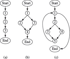
Figure 2.5 Sample control flow graphs to illustrate basis paths.

Table 2.2 Basis set and path vectors for the CFGs in Figure 2.5

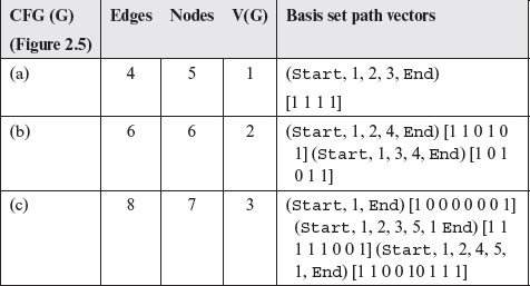
The number of basis paths is equal to the cyclomatic complexity of G. Recall from Chapter 1 that the cyclomatic complexity V(G) of a program with control graph G can be calculated by the following formula.

 

 

where e is the number of edges, n the number of nodes, and p the number of connected components in G.

Example 2.6   For each flow graph in Figure 2.5 the cyclomatic complexity, basis paths, and the corresponding path vectors are given in Table 2.2. The set of edges, and the corresponding sequencing of entries in the path vectors in this table are as follows.

Figure 2.5	Set of edges
(a)	{(Start, 1), (1, 2), (2, 3), (3, End)}
(b)	{Start, 1), (1, 2), (2, 4), (3, 4). (4,End)}
(c)	{Start, 1), (1, 2), (2, 3), (3, 5). (2, 4), (4, 5), (5, 1),(5,End)}

Exercises 2.3 through 2.6 ask you to derive basis sets for a few other programs.

2.2.5  Path conditions and domains

A path condition is a predicate that must evaluate to true for a path to be executed. For a straight line program having no conditional statements, the path condition is trivially true. However, for most programs, the path condition is a compound predicate obtained by conjoining the predicates along the path under consideration. A path condition partitions the input domain of a program. Thus, all inputs that satisfy the path condition are said to be in the path domain. The next example illustrates how to determine path conditions and hence the corresponding path domains.

 

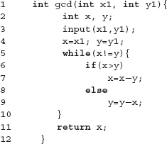
Example 2.7   Consider the following program that takes two non-negative integers x1 and y1 as inputs and computes their greatest common divisor.

The above program has an infinite number of paths one each for a set of pairs of integers. This set constitutes the domain of that path. Following is a list of a few paths through this program. These paths are labeled p₀, p₁₁, and p₁₂ where the first of the two indices denotes the number of times the loop is iterated and the second one indicates the variation within the loop due to the condition in the if statement.

Loop iterated zero times: p₀= (1, 2, 3, 4, 5, 11)

Loop iterated once:

For x > y: p₁₁: (1, 2, 3, 4, 5, 6, 7, 10, 5, 11)

For x ≤ y: p₁₂: (1, 2, 3, 4, 5, 6, 9, 10, 5, 11)

Note that each loop iteration leads to one additional path. This path depends on the code in the loop body. In the above example, the path could correspond to either the true or the false branch of the if statement.

 

A path domain can be computed by first finding the path conditions. The set of inputs that satisfy these conditions is the path domain for the path under consideration. For a program with no conditions the path domain is the input domain.

To determine the path domains, let us compute the condition associate with each path. Following are the conditions, and their simplified versions, for each of the three paths above.

p₀ : x1 = y1

p₁₁ : (x1 ≠ y1 ∧ (x1 – y1) = y1) → x1 = 2 ∗ y1

p₁₂ : (x1 ≠ y1 ∧ x1 = (y1 − x1)) → 2 ∗ x1 = y1

Note that each path condition is expressed in terms of the program inputs x1 and y1. Thus, for example, the first time the loop condition x ≠ y is evaluated, the values of program variables x and y are, respectively, x1 and y1. Hence the loop condition expressed in terms of input variables is x1 ≠ y1 and the corresponding path condition is x1 = y1. Similarly, the interpreted path conditions for P₁₁ and p₁₂ are, respectively, x1 = 2 ∗ y1 and 2 ∗ x1 = y1.

Expressing a condition along a path in terms of program input variables is known as interpretation of that condition. Obviously, the interpretation depends on the values of the program variables at the time the condition is evaluated.

Thus, the domain for path p₀ consists of all inputs for which x1 = y1. Similarly, the domains for the remaining two paths consist of all inputs that satisfy the corresponding conditions. Sample inputs in the domain of each of the three paths are given in the following as pairs of input integers.

p₀ : (4, 4), (10, 10)

p₁₁ : (4, 2), (8, 4)

p₁₂ : (4, 8), (5, 10)

 

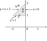
Example 2.8   Consider a program that takes two inputs denoted by integer variables x and y. Now consider the following sequence of three conditions that must evaluate to true in order for a path in this program to be executed.

y < x + 2

y > 1

x < 0

The above conditions define a path domain shown in Figure 2.6. Each of the above three conditions leads to a border segment, or simply border, shown as a darkened line and marked with an arrow. The path domain is the shaded area bounded by the three borders. All values of x and y that lie inside the domain will cause the path to be executed. Points that lie outside the domain or at the boundary will cause at least one of the above conditions to be false and hence the path will not be executed. For example, point c in the figure corresponds to (–0.5, 1). For this point the condition y > 1 is false.

 

Every path domain has a border along which lie useful tests.

Figure 2.6 Pictorial representation of a path domain corresponding to the condition y < x + 2 ∧ y > 1 ∧ x < 0. The shaded triangular area represents the path domain which is a subdomain of the entire program domain. Three sample points labeled a, b, and c, are shown. Point a lies inside the path domain, b lies outside, and c lies on one of the borders.

The path conditions in the above examples are linear and hence lead to straight line borders. Also, here we have assumed that the inputs are numbers, integers, or floating point values. In general, path condition dimensions could be arbitrary. Let relop = {<, ≤, >, ≥, =, ≠}. A general form of a set of m path conditions in n inputs x₁, x₂, . . . , x_n can be expressed as follows.

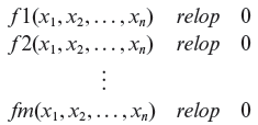
In case all functions in the above set of conditions are linear, the path conditions can be written as follows.

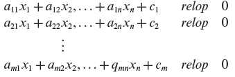
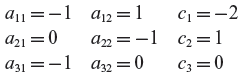
In the above conditions, a_ij denote the m × n coefficients of the input variables and c_j are m constants. Using the above standard notation, the path conditions in Example 2.8 can be expressed as follows.

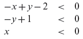
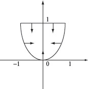
Figure 2.7 Non-linear path domain corresponding to the path condition y > x² ∧ y < 1. The arrows indicate the closed boundary of the parabolic domain.

In the above set of equations, the coefficients are given below.

Path conditions could also be non-linear. They could also contain arrays, strings, and other data types commonly found in programming languages. The next example illustrates a few other types of path conditions and the corresponding path domains.

 

Example 2.9   Consider the following two path conditions.

y − x²  >   0
y         <   1

Figure 2.7 is a graphical representation of the path domain that corresponds to the above conditions. The domain consists of points inside of a parabola bounded at the top by a line corresponding to the constraint y < 1.

Example 2.10   Often a condition in an if or a while loop contains reference to an array element. For instance, consider the following statements.

 

1   int x, n;

2   input (x, n);

3   inputArray(n, A);

4   . . . .

5   if(A[i]>x){

6   . . . .

 

The input domain of the above program consists of triples (x, n, A). The constraint A[i] > x defines a path domain consisting of all triples (x, n, Α′), where A′ is an array whose i^th element is greater than x. Of course, to define this domain more precisely one needs to know the range of variable i. Suppose that 0 ≤ i ≤ 10. In that case the path domain consists of all arrays of length 0 through 10 at least one of whose elements satisfies the path condition.

 

Just as in the case of arrays, it is often challenging to define path domains for abstract data types that occur in OO languages such as Java and C++. Consider, for example, a stack as used in the following program segment.

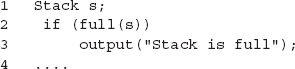
The path condition in the above program segment is full(s). Given stacks of arbitrary sizes, the path domain obviously consists of only stacks that are full. In situations like this, the program domain and the path domain are generally restricted for the purpose of testing by limiting stack size. Once done, one could consider stacks that are empty, full, or neither. Doing so partitions the program domain with respect to a stack into three subdomains one of which is a path domain.

That brings us to the end of this section to illustrate path conditions and path domains. Later in Chapter 4, we will see how to use path conditions to generate tests using a technique known as domain testing. (Also see Exercise 2.2.)

2.2.6  Domain and computation errors

Domain and computation errors are two error types based on the manner in which a program input leads to incorrect behavior. Specifically, a program P is said to contain a domain error if for a given input it follows a wrong path that leads to an incorrect output. P is said to contain a computation error if an input forces it to follow the correct path resulting in an incorrect output. An error in a predicate used in a conditional statement such as an if or a while leads to a domain error. An error in an assignment statement that computes a variable used later in a predicate may also lead to a domain error.

 

A domain error could occur because an incorrect path has been selected in which case it is considered as a path selection error. It could also occur due to a missing path in which case it is known as a missing path error. We shall return to the notion of domain errors in Chapter 4 while discussing domain testing as a technique for test data generation.

2.2.7  Static code analysis tools and static testing

A variety of questions related to code behavior are likely to arise during the code inspection process described briefly in Chapter 1. Consider the following example: A code inspector asks “Variable accel is used at line 42 in module updateAccel but where is it defined ?^,, The author might respond as “accel is defined in module computeAccel”. However, a static analysis tool could give a complete list of modules and line numbers where each variable is defined and used. Such a tool with a good user interface could simply answer the question mentioned above.

 

Static code analysis tools can provide control flow and data flow information. The control flow information, presented in terms of a CFG, is helpful to the inspection team in that it allows the determination of the flow of control under different conditions. A CFG can be annotated with data flow information to make a data flow graph. For example, to each node of a CFG, one can append the list of variables defined and used. This information is valuable to the inspection team in understanding the code as well as pointing out possible defects. Note that a static analysis tool might itself be able to discover several data flow related defects.

 

Several such commercial as well as open source tools are available. Purify from IBM Rational and Klockwork from Klockwork Inc. are two of the many commercially available tools for static analysis of C and Java programs. LAPSE (Lightweight Analysis for Program Security in Eclipse) is an open source tool for the analysis of Java programs.

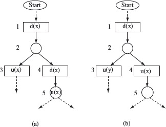
Example 2.11   Consider the CFGs in Figure 2.8 each of which has been annotated with data flow information. In (a) variable x is defined in block 1 and used subsequently in blocks 3 and 4. However, the CFG clearly shows that the definition of x at block 1 is used at block 3 but not at block 5. In fact the definition of x at block 1 is considered killed due to its redefinition at block 4.

Is the redefinition of x at block 5 an error ? The answer to this question depends on the function being computed by the code segment corresponding to the CFG. It is indeed possible that the redefinition at block 5 is erroneous. The inspection team must be able to answer this question with the help of the requirements and the static information obtained from an analysis tool.

Figure 2.8 Partial CFGs annotated with data flow information. d(x) and u(x), respectively, imply the definition and use of variable x in a block, (a) CFG that indicates a possible data flow error, (b) CFG with a data flow error.

Figure 2.8(b) indicates the use of variable y in block 3. If y is not defined along the path from Start to block 3, then there is a data flow error as a variable is used before it is defined. Several such errors can be detected by static analysis tools.

2.3  Execution History

Execution history of a program, also known as execution trace, is an organized collection of information about various elements of a program during a given execution. An execution slice is an executable sub-sequence of execution history. There are several ways to represent an execution history. For example, one possible representation is the sequence in which the functions in a program are executed against a given test input. Another representation is the sequence in which program blocks are executed. Thus, one could construct a variety of representations of the execution history of a program against a test input. For a program written in an object-oriented language like Java, an execution history could also be represented as a sequence of objects and the corresponding methods accessed.

 

Example 2.12   Consider Program P2.1 and its control flow graph in Figure 2.2 on page 78. We are interested in finding the sequence in which the basic blocks are executed when P2.1 is executed with the test input t₁ :< x = 2, y = 3 >. A straightforward examination of Figure 2.2 reveals the following sequence: 1, 3, 4, 5, 6, 5, 6, 5, 6, 7, 9. This sequence of blocks represents an execution history of P2.1 against test t₁. Another test t₂ :< x = 1, y = 0 > generates the following execution history expressed in terms of blocks: 1, 3, 4, 5, 7, 9.

An execution history may also include values of program variables. Obviously, the more the information in the execution history, the larger the space required to save it. What gets included or excluded from an execution history depends on its desired use and the space available for saving the history. For debugging a function, one might want to know the sequence of blocks executed as well as values of one or more variables used in the function. For selecting a subset of tests to run during regression testing, one might be satisfied with only a sequence of function calls or blocks executed. For performance analysis, one might be satisfied with a trace containing the sequence in which functions are executed. The trace is then used to compute the number of times each function is executed to assess its contribution to the total execution time of the program.

A complete execution history recorded from the start of a program’s execution until its termination represents a single execution path through the program. However, in some cases, such as during debugging, one might be interested only in partial execution history where program elements, such as blocks or values of variables, are recorded along a potion of the complete path. This portion might, for example, start when control enters a function of interest and end when the control exits this function.

2.4  Dominators and Post-Dominators

Let G = (Ν, E) be a control flow graph for program P. Recall that G has two special nodes labeled Start and End . We define the dominator and post-dominator as two relations on the set of nodes N. These relations find various applications, especially during the construction of tools for test adequacy assessment (Chapter 7) and regression testing (Chapter 9).

 

For nodes n and m in N, we say that n dominates m if n lies on every path from Start to m. We write dom(n, m) when n dominates m. In an analogous manner, we say that node n post-dominates node m if n lies on every path from m to the End node. We write pdom(n, m) when n post-dominates m. When n ≠ m, we refer to these as strict dominator and strict post-dominator relations. Dom(n) and PDom(n) denote, respectively the sets of dominators and post-dominators of node n.

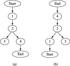
Figure 2.9 (a) Dominator and (b) post-dominator trees derived from the flow graph in Figure 2.4.

For n, m ∈ N, n is the immediate dominator of m when n is the last dominator of m along a path from the Start to m. We write idom(n, m) when n is the immediate dominator of m. Each node, except for Start, has a unique immediate dominator. Immediate dominators are useful in that we can use them to build a dominator tree. A dominator tree derived from G succinctly shows the dominator relation.

For n, m ∈ N, n is an immediate post-dominator of m if n is the first post-dominator along a path from m to End . Each node, except for End, has a unique immediate post-dominator. We write ipdom(n, m) when n is the immediate post-dominator of m. Immediate post-dominators allow us to construct a post-dominator tree that exhibits the post-dominator relation amongst the nodes in G.

Example 2.13   Consider the flow graph in Figure 2.4. This flow graph contains six nodes including Start and End. Its dominator and post-dominator trees are shown in Figure 2.9 (a) and (b), respectively. In the dominator tree, for example, a directed edge connects an immediate dominator to the node it dominates. Thus, among other relations, we have idom(1, 2) and idom(4, end). Similarly, from the post-dominator tree, we obtain ipdom(4, 2) and ipdom(End, 4).

Given a dominator and a post-dominator tree, it is easy to derive the set of dominators and post-dominators for any node. For example, the set of dominators for node 4, denoted as Dom(4) is {2, 1, Start}. Dom(4) is derived by first obtaining the immediate dominator of 4 which is 2, followed by the immediate dominator of 2 which is 1, and lastly the immediate dominator of 1, which is Start. Similarly, we can derive the set of post-dominators for node 2 as {4, End}.

2.5  Program Dependence Graph

A program dependence graph (PDG) for program P exhibits different kinds of dependencies amongst statements in P. For the purpose of testing, we consider data dependence and control dependence. These two dependencies are defined with respect to data and predicates in a program. Next we explain data and control dependence, how they are derived from a program, and their representation in the form of a PDG. We first show how to construct a PDG for programs with no procedures and then show how to handle programs with procedures.

 

2.5.1  Data dependence

Statements in a program exhibit a variety of dependencies. For example, consider Program P2.2. We say that the statement at line 8 depends on the statement at line 4 because line 8 may use the value of variable product defined at line 4. This form of dependence is known as data dependence.

Data dependence can be visually expressed in the form of a data dependence graph (DDG). A DDG for program P contains one unique node for each statement in P. Declaration statements are omitted when they do not lead to the initialization of variables. Each node in a DDG is labeled by the text of the statement as in a CFG or numbered corresponding to the program statement.

Two types of nodes are used: a predicate node is labeled by a predicate such as a condition in an if or a while statement and a data node labeled by an assignment, input, or output statement. A directed arc from node n₂ to n₁ indicates that node n₂ is data dependent on node n₁. This kind of data dependence is also known as flow dependence. A definition of data dependency follows.

 

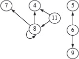
Example 2.14   Consider Program P2.2 and its data dependence graph in Figure 2.10. The graph shows seven nodes corresponding to the program statements. Data dependence is exhibited using directed edges. For example, node 8 is data dependent on nodes 4, 7, and itself because variable product is used at node 8 and defined at nodes 4 and 8, and variable num is used at node 8 and defined at node 7. Similarly, node 11 corresponding to the output statement, depends on nodes 4 and 8 because variable product is used at node 11 and defined at nodes 4 and 8.

Figure 2.10 Data dependence graph for Program P2.2. Node numbers correspond to line numbers. Declarations have been omitted.

Notice that the predicate node 6 is data dependent on nodes 5 and 9 because variable done is used at node 6 and defined through an input statement at nodes 5 and 9. We have omitted from the graph the declaration statements at lines 2 and 3 as the variables declared are defined in the input statements before use. To be complete, the data dependency graph could add nodes corresponding to these two declarations and add dependency edges to these nodes (see Exercise 2.7).

2.5.2  Control dependence

Another form of dependence is known as control dependence. For example, the statement at line 12 in Program P2.1 depends on the predicate at line 10. This is because control may or may not arrive at line 12 depending on the outcome of the predicate at line 10. Note that the statement at line 9 does not depend on the predicate at line 5 because control will arrive at line 9 regardless of the outcome of this predicate.

As with data dependence, control dependence can be visually represented as a control dependence graph (CDG). Each program statement corresponds to a unique node in the CDG. There is a directed edge from node n₂ to n₁ when n₂ is control dependent on n₁.

 

Example 2.15   Figure 2.11 shows the control dependence graph for P2.2. Control dependece edges are shown as dotted lines.

As shown, nodes 7, 8, and 9 are control dependent on node 6 because there exists a path from node 6 to each of the dependent nodes as well as a path that excludes these nodes. Notice that none of the remaining nodes is control dependent on node 6, the only predicate node in this example. Node 11 is not control dependent on node 6 because any path that goes from node 6 to program exit includes node 11.

Now that we know what data and control dependence is, we can show program dependence graph as a combination of the two dependences. Each program statement contains one node in the PDG. Nodes are joined with directed arcs showing data and control dependencies. A PDG can be considered as a combination of two subgraphs: a data dependence subgraph and a control dependence subgraph.

Example 2.16   Figure 2.12 shows the program dependence graph for P2.2. It is obtained by combining the graphs shown in Figures 2.10 and 2.11 (see Exercise 2.7).

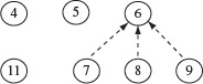
Figure 2.11 Control dependence graph for Program P2.2.

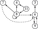
Figure 2.12 Program dependence graph for P2.2.

2.5.3  Call graph

As the name implies, a call graph is a directed graph in which each node is a call site, e.g., a procedure, and each edge connects two nodes (f, g) indicating that procedure f calls procedure g. For an object-oriented language such as C# or Java, a call graph captures calls to methods across objects.

 

A static call graph represents all potential procedure calls. A dynamic call graph captures calls that were actually made during one or more executions of the program. An exact static call graph is one that captures all potential call relationships. The problem of generating an exact static call graph is undecidable.

2.6  Strings, Languages, and Regular Expressions

Strings play an important role in testing. As we shall see in Section 5.2, strings serve as inputs to a finite state machine and hence to its implementation as a program. Thus, a string serves as a test input. A collection of strings also forms a language . For example, a set of all strings consisting of zeros and ones is the language of binary numbers. In this section we provide a brief introduction to strings and languages.

A collection of symbols is known as an alphabet. We will use an upper case letter such as X and Y to denote alphabets. Though alphabets can be infinite, we are concerned only with finite alphabets. For example, X = {0,1} is an alphabet consisting of two symbols 0 and 1. Another alphabet is Y = {dog, cat, horse, lion} that consists of four symbols “dog”, “cat”, “horse”, and “lion”.

 

A string over an alphabet X is any sequence of zero or more symbols that belong to X. For example, 0110 is a string over the alphabet {0, 1}. Also, dog cat dog dog lion is a string over the alphabet {dog, cat, horse, lion}. We will use lower case letters such as p, q, r to denote strings. The length of a string is the number of symbols in that string. Given a string s, we denote its length by |s|. Thus, |1011| =4 and |dogcatdog| = 3. A string of length 0, also known as an empty string, is denoted by ∈.

Let s₁ and s₂ be two strings over alphabet X. We write s₁ • s₂ to denote the concatenation of strings s₁ and s₂. For example, given the alphabet X = {0,1}, and two strings 011 and 101 over X, we obtain 011•101 = 011101. It is easy to see that |s₁ • s₂| = |s₁| + |s₂|. Also, for any string s, we have s • ∈ = s and ∈ • s = s.

A set L of strings over an alphabet X is known as a language. A language can be finite or infinite. Given languages L₁ and L₂, we denote their catenation as L₁ • L₂ that denotes the set L defined as:

 

L = L₁ • L₂ = {x • y|x ∈ L₁, y ∈ L₂}

 

The following sets are finite languages over the binary alphabet {0,1}.

 

∅: The empty set

{∈}: A language consisting only of one string of length zero

{00, 11, 0101}: A language containing three strings

 

A regular expression is a convenient means for a compact representation of sets of strings. For example, the regular expression (01)* denotes the set of strings that consists of the empty string, the string 01, and all strings obtaining by concatenating the string 01 with itself one or more times. Note that (01)* denotes an infinite set. A formal definition of regular expressions follows.

Regular Expressions

Given a finite alphabet X, the following are regular expressions over X:

• If a belongs to X, then a is a regular expression that denotes the set {a}.
• Let r₁ and r₂ be regular expressions over the alphabet X that denote, respectively, sets L₁ and L₂. Then r₁ • r₂ is a regular expression that denotes the set L₁• L₂.
• If r is a regular expression that denotes the set L, then r+ is a regular expression that denotes the set obtained by concatenating L with itself one or more times also written as L⁺. Also, r^*, known as the Kleene closure of r, is a regular expression. If r denotes the set L then r* denotes the set {∈} ∪ L⁺.
• If r₁ and r₂ are regular expressions that denote, respectively, sets L₁ and L₂, then r₁|r₂ is also a regular expression that denotes the set L₁∪L₂.

Regular expressions are useful in expressing both finite and infinite test sequences. For example, if a program takes a sequence of zeroes and ones and flips each zero to a 1 and a 1 to a 0, then a few possible sets of test inputs are 0*, (10)+, 010|100.

2.7  Tools

A large variety of tools are available for static analysis of code in various languages. Below is a sample of such tools.

Tool: EclipseCFG

Link: http://eclipsefcg.sourceforge.net/

Description

EclipseCFG is an Eclipse plugin for generating CFG for Java code. The CFG is generated for each method in the selected class. The CodeCover tool is integrated with Eclipse and EclipseCFG. This integration enables the CFG to graphically indicate statement and condition coverage. The tool also computes the McCabe complexity metric for each method.

Tool: LDRS Testbed.

Link: http://www.ldra.com/index.php/en/products-a-services/ldra-tool-suite/ldra-testbedr

Description

This is a commercial-strength static and dynamic analysis tool set. It analyzes the source code statically by doing a complete syntax analysis either for individual functions or for the entire system. The tool provides statement, branch, and MC/DC coverage. Hence, this tool is useful in environments that develop code that must meet DO-178B certification. The coverage results are displayed in a tabular form and can also be viewed in the form of a dynamic call graph.

Tool: CodeSonar

Link: http://www.grammatech.com/products/codesonar/support.html

Description

CodeSonar is a static analysis tool for C and C++ programs. It attempts to detect several problems in the code including data races, deadlocks, buffer overruns, and memory usage after it has been freed. It also includes a powerful feature for application architecture visualization.

Tool: gprof

Link: http://sourceware.org/binutils/docs/gprof/

Description

gprof is a profiler to collect run time statistics of a program. It generates a dynamic call graph of a program. The call graph is presented in textual form.

Exercises

2.1(a) Calculate the length of the path traversed when P2.2 is executed on an input sequence containing Ν integers. (b) Suppose that the statement on line 8 of P2.2 is replaced by the following.
8 if(num>0)product=product∗num:
Calculate the number of distinct paths in the modified P2.2 if the length of the input sequence can be 0, 1, or 2. (c) For an input sequence of length N, what is the maximum length of the path traversed by the modified P2.2 ?

2.2 (a) List the different paths in the program in Example 2.7 when the loop body is traversed twice. (b) For each path list the path conditions and a few sample values in the corresponding input domain.

2.3 Find the basis set and the corresponding path vectors for the flow graph in Figure 2.2. Construct a path p through this flow graph that is not a basis path. Find the path vector V_p for p. Express V_p as a linear combination of the path vectors for the basis paths.

2.4 Solve Exercise 2.7 but for the program in Example 2.7.

2.5 Let P denote a program that contains a total of n simple conditions in if and while statements. What is the maximum number of elements in the basis set for P? What is the largest path vector in P?

2.6 The basis set for a program is constructed using its CFG. Now suppose that the program contains compound predicates. Do you think the basis set for this program will depend on how compound predicates are represented in the flow graph? Explain your answer.

2.7 Construct the dominator and post-dominator trees for the control flow graph in Figure 2.2 and for each of the control flow graphs in Figure 2.13.

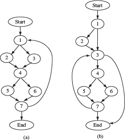
Figure 2.13 Control flow graphs for Exercise 2.7.

2.8 Let pred(n) be the set of all predecessors of node n in a CFG G=(N, E). The set of dominators of n can be computed using the following equations:

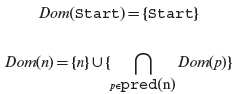
Using the above equation, develop an algorithm to compute the dominators of each node in N. (Note: There exist several algorithms for computing the dominators and post-dominators in a CFG. Try developing your own and then study the algorithms in relevant citations in the Bibliography.)

2.9 (a) Modify the dependence graph in Figure 2.10 by adding nodes corresponding to the declarations at lines 2 and 3 in Program P2.2 and the corresponding dependence edges. (b) Can you offer a reason why for Program P2.2 the addition of nodes corresponding to the declarations is redundant ? (c) Under what condition would it be useful to add nodes corresponding to declarations to the data dependence graph ?

2.10 Construct a program dependence graph for the exponentiation program P2.1.

2.11 What is the implication of a cycle in a call graph?