1
Inner Product Spaces (Pre-Hilbert)
This chapter will focus on inner product spaces, that is, vector spaces with a scalar product, specifically those of finite dimension.
1.1. Real and complex inner products
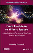
In real Euclidean spaces ℝ2 and ℝ3, the inner product of two vectors v, w is defined as the real number:
where ϑ is the smallest angle between v and w and ‖ ‖ represents the norm (or the magnitude) of the vectors.
Using the inner product, it is possible to define the orthogonal projection of vector v in the direction defined by vector w. A distinction must be made between:
- – the scalar projection of v in the direction of
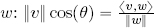 ; and
; and - – the vector projection of v in the direction of
 ;
;
where ![]() is the unit vector in the direction of w. Evidently, the roles of v and w can be reversed.
is the unit vector in the direction of w. Evidently, the roles of v and w can be reversed.
The absolute value of the scalar projection measures the “similarity” of the directions of two vectors. To understand this concept, consider two remarkable relative positions between v and w:
- – if v and w possess the same direction, then the angle between them ϑ is either null or π, hence cos(ϑ) = ±1, that is, the absolute value of the scalar projection of v in direction w is ‖v‖;
- – however, if v and w are perpendicular, then
 and hence cos(ϑ) = 0, showing that the scalar projection of v in direction w is null.
When the position of v relative to w falls somewhere in the interval between the two vectors described above, the absolute value of the scalar projection of v in the direction of w falls between 0 and ‖v‖; this explains its use to measure the similarity of the direction of vectors.
In this book, we shall consider vector spaces which are far more complex than ℝ2 and ℝ3, and the measure of vector similarity obtained through projection supplies crucial information concerning the coherence of directions.
Before we can obtain this information, we must begin by moving from Euclidean spaces ℝ2 and ℝ3 to abstract vector spaces. The general definition of an inner product and an orthogonal projection in these spaces may be seen as an extension of the previous definitions, permitting their application to spaces in which our representation of vectors is no longer applicable.
Geometric properties, which can only be apprehended and, notably, visualized in two or three dimensions, must be replaced by a set of algebraic properties which can be used in any dimension.
Evidently, these algebraic properties must be necessary and sufficient to characterize the inner product of vectors in a plane or in real space. This approach, in which we generalize concepts which are “intuitive” in two or three dimensions, is a classic approach in mathematics.
In this chapter, the symbol V will be used to describe a vector space defined over the field ![]() , where
, where ![]() is either ℝ or
is either ℝ or ![]() and is of finite dimension n < +∞. field
and is of finite dimension n < +∞. field ![]() contains the scalars used to construct linear combinations between vectors in V . Note that two finite dimensional vector spaces are isomorphic if and only if they are of the same dimension. Furthermore, if we establish a basis B = (b1, . . . , bn) for V , an isomorphism between V and
contains the scalars used to construct linear combinations between vectors in V . Note that two finite dimensional vector spaces are isomorphic if and only if they are of the same dimension. Furthermore, if we establish a basis B = (b1, . . . , bn) for V , an isomorphism between V and ![]() n can be constructed as follows:
n can be constructed as follows:

that is, I associates each v ∈ V with the vector of ![]() n given by the scalar components of v in relation to the established basis B. Since I is an isomorphism, it follows that
n given by the scalar components of v in relation to the established basis B. Since I is an isomorphism, it follows that ![]() n is the prototype of all vector spaces of dimension n over a field
n is the prototype of all vector spaces of dimension n over a field ![]() .
.
DEFINITION 1.1.– Let V be a vector space defined over a field ![]() .
.
A ![]() -form over V is an application defined over V × V with values in
-form over V is an application defined over V × V with values in ![]() , that is:
, that is:
DEFINITION 1.2.– Let V be a real vector space. A couple (V, 〈, 〉) is said to be a real inner product space (or a real pre-Hilbert space) if the form 〈, 〉 is:
1) bilinear, i.e.1 linear in relation to each argument (the other being fixed):
and:
2) symmetrical: 〈v, w〉 = 〈w, v〉, ∀v, w ∈ V ;
3) defined: 〈v, v〉 = 0 ![]() v = 0V , the null vector of the vector space V ;
v = 0V , the null vector of the vector space V ;
4) positive: 〈v, v〉 > 0 ∀v ∈ V , v ≠ 0V .
Upon reflection, we see that, for a real form over V , the symmetry and bilinearity requirements are equivalent to requiring symmetry and linearity on the left-hand side, that is:
The simplest and most important example of a real inner product is the canonical inner product, defined as follows: let v = (v1, v2, . . . , vn), w = (w1, w2, . . . , wn) be two vectors in ℝn written with their components in relation to any given, but fixed, basis ![]() in ℝn. The canonical inner product of v and w is:
in ℝn. The canonical inner product of v and w is:
where vt and wt in the final equations are the transposed vectors of v and w, giving us the matrix product of a line vector (treated as a 1 × n matrix) and a column vector (treated as an n × 1 matrix).
The extension of these definitions to complex vector spaces is not particularly straightforward. First, note that if V is a complex vector space, then there is no bilinear and definite-positive transformation over V × V . In this case, any vector v ∈ V would give the following:
As we shall see, the property of positivity is essential in order to define a norm (and thus a distance, and by extension, a topology) from a complex inner product. To obtain an algebraic structure for complex scalar products which remains compatible with a topological structure, we are therefore forced to abandon the notion of bilinearity, and to search for an alternative.
We could consider antilinearity2, i.e.
But it has the same problem as bilinearity, 〈iv, iv〉 = (−i)(−i)〈v, v〉 = i2〈v, v〉 = −〈v, v〉2 ≼ 0.
A simple analysis shows that, in order to avoid losing the positivity, it is sufficient to request the linearity with respect to one variable and the antilinearity with respect to the other. This property is called sesquilinearity3.
The choice of the linear and antilinear variable is entirely arbitrary.
By convention, the antilinear component is placed on the right-hand side in mathematics, but on the left-hand side in physics.
We have chosen to adopt the mathematical convention here, i.e. 〈αv, βw〉 = αβ̅〈v, w〉.
Next, it is important to note that sesquilinearity and symmetry are incompatible: if both properties were verified, then 〈v, αw〉 = ![]() 〈v, w〉, and also 〈v, αw〉 = 〈αw, v〉 = α〈w, v〉 = α〈v, w〉. Thus, 〈v, αw〉 =
〈v, w〉, and also 〈v, αw〉 = 〈αw, v〉 = α〈w, v〉 = α〈v, w〉. Thus, 〈v, αw〉 = ![]() 〈v, w〉 = α〈v, w〉 which can only be verified if α ∈ ℝ.
〈v, w〉 = α〈v, w〉 which can only be verified if α ∈ ℝ.
Thus 〈, 〉 cannot be both sesquilinear and symmetrical when working with vectors belonging to a complex vector space.
The example shown above demonstrates that, instead of symmetry, the property which must be verified for every vector pair v, w is ![]() , that is, changing the order of the vectors in 〈, 〉 must be equivalent to complex conjugation.
, that is, changing the order of the vectors in 〈, 〉 must be equivalent to complex conjugation.
A transform which verifies this property is said to be Hermitian4.
These observations provide full justification for Definition 1.3.
DEFINITION 1.3.– Let V be a complex vector space. The pair (V, 〈, 〉) is said to be a complex inner product space (or a complex pre-Hilbert space) if 〈, 〉 is a complex form which is:
1) sesquilinear:
∀ v1, v2, w1, w2 ∈ V , and:
∀ α, β ∈ ![]() , ∀ v, w ∈ V ;
, ∀ v, w ∈ V ;
2) Hermitian: ![]() , ∀v, w ∈ V ;
, ∀v, w ∈ V ;
3) definite: 〈v, v〉 = 0 ![]() v = 0V , the null vector of the vector space V;
v = 0V , the null vector of the vector space V;
4) positive: 〈v, v〉 > 0 ∀v ∈ V , v ≠ 0V .
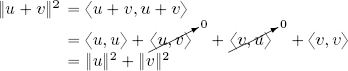
As in the case of the canonical inner product, for a complex form over V , the symmetry and sesquilinearity requirement is equivalent to requiring the Hermitian property and linearity on the left-hand side; if these properties are verified, then:
Considering the sum of n, rather than two, vectors, sesquilinearity is represented by the following formulae:
In ![]() n, the complex Euclidean inner product is defined by:
n, the complex Euclidean inner product is defined by:
where v = (v1, v2, . . . , vn), w = (w1, w2, . . . , wn) ∈ ![]() n are written with their components in relation to any given, but fixed, basis
n are written with their components in relation to any given, but fixed, basis ![]() in
in ![]() n.
n.
The symbol ![]() will be used throughout to represent either ℝ or
will be used throughout to represent either ℝ or ![]() in the context of properties which are valid independently of the reality or complexity of the inner product.
in the context of properties which are valid independently of the reality or complexity of the inner product.
THEOREM 1.1.– Let (V, 〈 , 〉) be an inner product space. We have:
1) 〈v, 0V 〉 = 0 ∀v ∈ V ;
2) if 〈u, w〉 = 〈v, w〉 ∀w ∈ V , then u and v must coincide;
3) 〈v, w〉 = 0 ∀v ∈ V ![]() w = 0V , i.e. the null vector is the only vector which is orthogonal to all of the other vectors.
w = 0V , i.e. the null vector is the only vector which is orthogonal to all of the other vectors.
PROOF.–
1) 〈v, 0V 〉 = 〈v, 0V + 0V 〉 = 〈v, 0V 〉 + 〈v, 0V 〉 by linearity, i.e. 〈v, 0V 〉 − 〈v, 0V 〉 = 0 = 〈v, 0V 〉.
2) 〈u, w〉 = 〈v, w〉 ∀w ∈ V implies, by linearity, that 〈u − v, w〉 = 0 ∀w ∈ V and thus, notably, considering w = u − v, we obtain 〈u − v, u − v〉 = 0, implying, due to the definite positiveness of the inner product, that u − v = 0V , i.e. u = v.
3) If w = 0V , then 〈v, w〉 = 0 ∀v ∈ V using property (1). Inversely, by hypothesis, it holds that 〈v, w〉 = 0 = 〈v, 0V 〉 ∀v ∈ V , but then property (2) implies that w = 0V .
Finally, let us consider a typical property of the complex inner product, which results directly from a property of complex numbers.
THEOREM 1.2.– Let (V, 〈 , 〉) be a complex inner product space. Thus:
PROOF.– Consider any complex number z = a + ib, so −iz = b − ia, hence b = ℑ (z) = ℜ (−iz). Taking z = 〈v, w〉, we obtain ℑ (〈v, w〉) = ℜ (−i〈v, w〉) = ℜ (〈v, iw〉) by sesquilinearity.
1.2. The norm associated with an inner product and normed vector spaces
If (V, 〈, 〉) is an inner product space over ![]() , then a norm on V can be defined as follows:
, then a norm on V can be defined as follows:
Note that ‖v‖ is well defined since 〈v, v〉 ≽ 0 ∀v ∈ V . Once a norm has been established, it is always possible to define a distance between two vectors v, w in V : d(v, w) = ‖v − w‖.
The vector v ∈ V such that ‖v‖= 1 is known as a unit vector. Every vector v ∈ V can be normalized to produce a unit vector, simply by dividing it by its norm.
Three properties of the norm, which should already be known, are listed below. Taking any v, w ∈ V , and any α ∈ ![]() :
:
1) ‖v‖≽ 0, ‖v‖= 0 ![]() v = 0V ;
v = 0V ;
2) ‖αv‖= |α|‖v‖(homogeneity);
3) ‖v + w‖≼ ‖v‖+ ‖w‖(triangle inequality).
DEFINITION 1.4 (normed vector space).– A normed vector space is a pair (V, ‖ ‖) given by a vector space V and a function, called a norm, ![]() , satisfying the three properties listed above.
, satisfying the three properties listed above.
A norm ‖ ‖ is Hilbertian if there exists an inner product 〈 , 〉 on V such that ![]() .
.
Canonically, an inner product space is therefore a normed vector space. Counterexamples can be used to show that the reverse is not generally true.
Note that, by definition, 〈v, v〉 = ‖v‖ ‖v‖, but, in general, the magnitude of the inner product between two different vectors is dominated by the product of their norms. This is the result of the well-known inequality shown below.
THEOREM 1.3 (Cauchy-Schwarz inequality).– For all v, w ∈ (V, 〈 , 〉) we have:
PROOF.– Dozens of proofs of the Cauchy-Schwarz inequality have been produced. One of the most elegant proofs is shown below, followed by the simplest one:
– first proof: if w = 0V , then the inequality is verified trivially with 0 = 0. If w ≠ 0V , then we can define ![]() , i.e.
, i.e. ![]() and we note that:
and we note that:
thus:

as the two intermediate terms in the penultimate step are zero, since 〈z, w〉 = 〈w, z〉 = 0.
As ‖z‖2 ≽ 0, we have seen that:
i.e. |〈v, w〉|2 ≼ ‖v‖2‖w‖2, hence |〈v, w〉| ≼ ‖v‖‖w‖;
– second proof (in one line!): ∀t ∈ ℝ we have:
The Cauchy-Schwarz inequality allows the concept of the angle between two vectors to be generalized for abstract vector spaces. In fact, it implies the existence of a coefficient k between −1 and +1 such that 〈v, w〉 = ‖v‖‖w‖k, but, given that the restriction of cos to [0, π] creates a bijection with [−1, 1], this means that there is only one ϑ ∈ [0, π] such that 〈v, w〉 = ‖v‖‖w‖ cos ϑ. ϑ ∈ [0, π] is known as the angle between the two vectors v and w.
Another very important property of the norm is as follows.
THEOREM 1.4.– Let (V, ‖ ‖) be an arbitrary normed vector space and v, w ∈ V . We have:
PROOF.– On one side:
by the triangle inequality, thus ‖v‖ − ‖w‖ ≼ ‖v − w‖. On the other side:
thus ‖w‖ − ‖v‖ ≼ ‖v − w‖, i.e. ‖v‖ − ‖w‖ ≽ − ‖v − w‖.
Hence, −‖v − w‖ ≼ ‖v‖ − ‖w‖ ≼ ‖v − w‖, i.e. |‖v‖ − ‖w‖| ≼ ‖v − w‖.
The following formula is also extremely useful.
THEOREM 1.5 (Carnot’s theorem).– Taking v, w ∈ (V, 〈 , 〉):
and
PROOF.– Direct calculation:
If ![]() =
= ![]() , then
, then ![]() , and since, if z = a + ib = ℜ (z) + iℑ(z), then z +
, and since, if z = a + ib = ℜ (z) + iℑ(z), then z + ![]() = 2a = 2ℜ(z), we can rewrite [1.5] as:
= 2a = 2ℜ(z), we can rewrite [1.5] as:
The laws presented in this section have immediate consequences which will be highlighted in section 1.2.1.
1.2.1. The parallelogram law and the polarization formula
The parallelogram law in ℝ2 is shown in Figure 1.1. This law can be generalized on a vector space with an arbitrary inner product.
THEOREM 1.6 (Parallelogram law).– Let (V, 〈, 〉) be an inner product space on ![]() . Thus, ∀v, w ∈ V :
. Thus, ∀v, w ∈ V :

Figure 1.1. Parallelogram law in ℝ2: The sum of the squares of the two diagonal lines is equal to two times the sum of the squares of the edges v and w. For a color version of this figure, see www.iste.co.uk/provenzi/spaces.zip
PROOF.– A direct consequence of law [1.4] or law [1.5] taking ‖v + w‖2 then ‖v − w‖2.
□
As we have seen, an inner product induces a norm. The polarization formula can be used to “reverse” roles and write the inner product using the norm.
THEOREM 1.7 (Polarization formula).– Let (V, 〈, 〉) be an inner product space on ![]() . In this case, ∀v, w ∈ V :
. In this case, ∀v, w ∈ V :
and:
PROOF.– This law is a direct consequence of law [1.4], in the real case. For the complex case, w is replaced by iw in law [1.5], and by sesquilinearity, we obtain:
By direct calculation, we can then verify that ‖v + w‖2 − ‖v − w‖2 + i ‖v + iw‖2 − i ‖v − iw‖2 = 4〈v, w〉.
It may seem surprising that something as simple as the parallelogram law may be used to establish a necessary and sufficient condition to guarantee that a norm over a vector space will be induced by an inner product, that is, the norm is Hilbertian. This notion will be formalized in Chapter 4.
1.3. Orthogonal and orthonormal families in inner product spaces
The “geometric” definition of an inner product in ℝ2 and ℝ3 indicates that this product is zero if and only if ϑ, the angle between the vectors, is π/2, which implies cos(ϑ) = 0.
In more complicated vector spaces (e.g. polynomial spaces), or even Euclidean vector spaces of more than three dimensions, it is no longer possible to visualize vectors; their orthogonality must therefore be “axiomatized” via the nullity of their scalar product.
DEFINITION 1.5.– Let (V, 〈, 〉) be a real or complex inner product space of finite dimension n. Let F = {v1, · · · , vn} be a family of vectors in V . Thus:
– F is an orthogonal family of vectors if each different vector pair has an inner product of 0: 〈vi, vj〉 = 0;
– F is an orthonormal family if it is orthogonal and, furthermore, ‖vi‖ = 1 ∀i. Thus, if ![]() is an orthogonal family,
is an orthogonal family, ![]() is an orthonormal family.
is an orthonormal family.
An orthonormal family (unit and orthogonal vectors) may be characterized as follows:

δi,j is the Kronecker delta5.
1.4. Generalized Pythagorean theorem
The Pythagorean theorem can be generalized to abstract inner product spaces. The general formulation of this theorem is obtained using a lemma.
LEMMA 1.1.– Let (V, 〈, 〉) be a real or complex inner product space. Let u ∈ V be orthogonal to all vectors v1, . . . , vn ∈ V . Hence, u is also orthogonal to all vectors in V obtained as a linear combination of v1, . . . , vn.
PROOF.– Let ![]() , be an arbitrary linear combination of vectors v1, . . . , vn. By direct calculation:
, be an arbitrary linear combination of vectors v1, . . . , vn. By direct calculation:
THEOREM 1.8 (Generalized Pythagorean theorem).– Let (V, 〈, 〉) be an inner product space on ![]() . Let u, v ∈ V be orthogonal to each other. Hence:
. Let u, v ∈ V be orthogonal to each other. Hence:
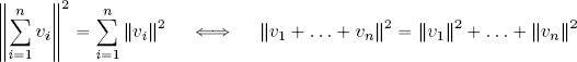
More generally, if the vectors v1,. . . , vn ∈ V are orthogonal, then:
PROOF.– The two-vector case can be proven thanks to Carnot’s formula:
Proof for cases with n vectors is obtained by recursion:
– the case where n = 2 is demonstrated above;
– we suppose that ![]() (recursion hypothesis);
(recursion hypothesis);
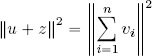
– now, we write u = vn and ![]() , so u ⊥ z using Lemma 1.1. Hence, using case n = 2: ‖u + z‖2 = ‖u‖2 + ‖z‖2, but:
, so u ⊥ z using Lemma 1.1. Hence, using case n = 2: ‖u + z‖2 = ‖u‖2 + ‖z‖2, but:
so:
and:

giving us the desired thesis.
Note that the Pythagorean theorem thesis is a double implication if and only if V is real, in fact, using law [1.6] we have that ‖u + v‖2 = ‖u‖2 + ‖v‖2 holds true if and only if ℜ(〈u, v〉) = 0, which is equivalent to orthogonality if and only if V is real.
The following result gives information concerning the distance between any two vectors within an orthonormal family.
THEOREM 1.9.– Let (V, 〈, 〉) be an inner product space on ![]() and let F be an orthonormal family in V . The distance between any two elements of F is constant and equal to
and let F be an orthonormal family in V . The distance between any two elements of F is constant and equal to ![]() .
.
PROOF.– Using the Pythagorean theorem: ‖u + (−v)‖2 = ‖u‖2 + ‖v‖2 = 2, from the fact that u ⊥ v.□
1.5. Orthogonality and linear independence
The orthogonality condition is more restrictive than that of linear independence: all orthogonal families are free.
THEOREM 1.10.– Let F be an orthogonal family in (V, 〈, 〉), F = {v1, · · · , vn}, vi ≠ 0 ∀i, then F is free.
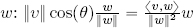
PROOF.– We need to prove the linear independence of the elements vi, that is, ![]() . To this end, we calculate the inner product of the linear combination
. To this end, we calculate the inner product of the linear combination ![]() and an arbitrary vector vj with j ∈ {1, . . . , n}:
and an arbitrary vector vj with j ∈ {1, . . . , n}:
By hypothesis, none of the vectors in F are zero; the hypothesis that ![]() therefore implies that:
therefore implies that:
This holds for any j ∈ {1, . . . , n}, so the orthogonal family F is free.□
Using the general theory of vector spaces in finite dimensions, an immediate corollary can be derived from theorem 1.10.
COROLLARY 1.1.– An orthogonal family of n non-null vectors in a space (V, 〈, 〉) of dimension n is a basis of V .
DEFINITION 1.6.– A family of n non-null orthogonal vectors in a vector space (V, 〈, 〉) of dimension n is said to be an orthogonal basis of V . If this family is also orthonormal, it is said to be an orthonormal basis of V .
The extension of the orthogonal basis concept to inner product spaces of infinite dimensions will be discussed in Chapter 5. For the moment, it is important to note that an orthogonal basis is made up of the maximum number of mutually orthogonal vectors in a vector space. Taking n to represent the dimension of the space V and proceeding by reductio ad absurdum, imagine the existence of another vector u* ∈ V , u ≠ 0, orthogonal to all of the vectors in an orthogonal basis ![]() ; in this case, the set
; in this case, the set ![]() would be free as orthogonal vectors are linearly independent, and the dimension of V would be n + 1 instead of n! This property is usually expressed by saying that an orthogonal family is a basis if it is not a subset of another orthogonal family of vectors in V .
would be free as orthogonal vectors are linearly independent, and the dimension of V would be n + 1 instead of n! This property is usually expressed by saying that an orthogonal family is a basis if it is not a subset of another orthogonal family of vectors in V .
Note that in order to determine the components of a vector in relation to an arbitrary basis, we must solve a linear system of n equations with n unknown variables. In fact, if v ∈ V is any vector and (ui) i = 1, . . . , n is a basis of V , then the components of v in (ui) are the scalars α1, . . . , αn such that:

where ui,j is the j-th component of vector ui.
However, in the presence of an orthogonal or orthonormal basis, components are determined by inner products, as seen in Theorem 1.11.
Note, too, that solving a linear system of n equations with n unknown variables generally involves far more operations than the calculation of inner products; this highlights one advantage of having an orthogonal basis for a vector space.
THEOREM 1.11.– Let B = {u1, . . . , un} be an orthogonal basis of (V, 〈, 〉). Then:
Notably, if B is an orthonormal basis, then:
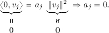
PROOF.– B is a basis, so there exists a set of scalars α1, . . . , αn such that ![]() . Consider the inner product of this expression of v with a fixed vector ui, i ∈ {1, . . . , n}:
. Consider the inner product of this expression of v with a fixed vector ui, i ∈ {1, . . . , n}:
so ![]() , and thus
, and thus ![]() . If B is an orthonormal basis, ‖ui‖ = 1 giving the second law in the theorem.□
. If B is an orthonormal basis, ‖ui‖ = 1 giving the second law in the theorem.□
Geometric interpretation of the theorem: The theorem that we are about to demonstrate is the generalization of the decomposition theorem of a vector in plane ℝ2 or in space ℝ3 on a canonical basis of unit vectors on axes. To simplify this, consider the case of ℝ2.
If ![]() and
and ![]() are, respectively, the unit vectors of axes x and y, then the decomposition theorem says that:
are, respectively, the unit vectors of axes x and y, then the decomposition theorem says that:
which is a particular case of the theorem above.
We will see that the Fourier series can be viewed as a further generalization of the decomposition theorem on an orthogonal or orthonormal basis.
1.6. Orthogonal projection in inner product spaces
The definition of orthogonal projection can be extended by examining the geometric and algebraic properties of this operation in ℝ2 and ℝ3. Let us begin with ℝ2.
In the Euclidean space ℝ2, the inner product of a vector v and a unit vector evidently gives us the orthogonal projection of v in the direction defined by this vector, as shown in Figure 1.2 with an orthogonal projection along the x axis.
The properties verified by this projection are as follows:
1) projecting onto the x axis a second time, vector Pxv obviously remains unchanged given that it is already on the x axis, i.e. ![]() . Put differently, the operator Px bound to the x axis is the identity of this axis;
. Put differently, the operator Px bound to the x axis is the identity of this axis;
2) the difference vector between v and its projection v − Pxv is orthogonal to the x axis, as we see from Figure 1.3;
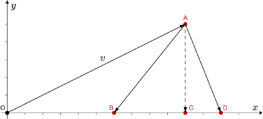
Figure 1.2. Orthogonal projection  and diagonal projections
  and
and  of a vector in v ∈ ℝ2 onto the x axis. For a color version of this figure, see www.iste.co.uk/provenzi/spaces.zip
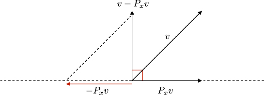
Figure 1.3. Visualization of property 2 in ℝ2. For a color version of this figure, see www.iste.co.uk/provenzi/spaces.zip
3) Pxv minimizes the distance between the terminal point of v and the x axis. In Figure 1.2, ![]() and
and ![]() are, in fact, the hypotenuses of right-angled triangles ABC and ACD; on the other hand,
are, in fact, the hypotenuses of right-angled triangles ABC and ACD; on the other hand, ![]() is another side of these triangles, and is therefore smaller than
is another side of these triangles, and is therefore smaller than ![]() and
and ![]() .
. ![]() is the distance between the terminal point of v and the terminal point of Pxv, while
is the distance between the terminal point of v and the terminal point of Pxv, while ![]() and
and ![]() are the distances between the terminal point of v and the diagonal projections of v onto x rooted at B and D, respectively.
are the distances between the terminal point of v and the diagonal projections of v onto x rooted at B and D, respectively.
We wish to define an orthogonal projection operation for an abstract inner product space of dimension n which retains these same geometric properties.
Analyzing orthogonal projections in ℝ3 helps us to establish an idea of the algebraic definition of this operation. Figure 1.4 shows a vector v ∈ ℝ3 and the plane produced by the orthogonal vectors u1 and u2. We see that the projection p of v onto this plane is the vector sum of the orthogonal projections ![]() and
and ![]() onto the two vectors u1 and u2 taken separately, i.e.
onto the two vectors u1 and u2 taken separately, i.e. ![]() .
.

Figure 1.4. Orthogonal projection p of a vector in ℝ3 onto the plane produced by two unit vectors. For a color version of this figure, see www.iste.co.uk/provenzi/spaces.zip
Generalization should now be straightforward: consider an inner product space (V, 〈, 〉) of dimension n and an orthogonal family of non-zero vectors F = {u1, . . . , um}, m ≼ n, ui ≠ 0V ∀i = 1, . . . , m.
The vector subspace of V produced by all linear combinations of the vectors of F shall be written Span(F ):

The orthogonal projection operator or orthogonal projector of a vector v ∈ V onto S is defined as the following application, which is obviously linear:

Theorem 1.12 shows that the orthogonal projection defined above retains all of the properties of the orthogonal projection demonstrated for ℝ2.
THEOREM 1.12.– Using the same notation as before, we have:
1) if s ∈ S then PS(s) = s, i.e. the action of PS on the vectors in S is the identity;
2) ∀v ∈ V and s ∈ S, the residual vector of the projection, i.e. v − PS(v), is ⊥ to S:
3) ∀v ∈ V et s ∈ S: ‖v − PS(v)‖ ≼ ‖v − s‖ and the equality holds if and only if s = PS(v). We write:
PROOF.–
1) Let s ∈ S, i.e. ![]() , then:
, then:
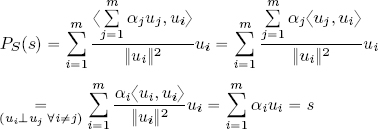
2) Consider the inner product of PS(v) and a fixed vector uj, j ∈ {1, . . . , m}:
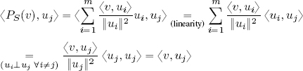
hence:
Lemma 1.1 guarantees that ![]() .
.
3) It is helpful to rewrite the difference v − s as v − PS(v) + PS(v) − s. From property 2, v−PS(v)⊥S, however PS(v), s ∈ S so PS(v)−s ∈ S. Hence (v−PS(v)) ⊥ (PS(v) − s). The generalized Pythagorean theorem implies that:
hence ‖v − s‖ ≽ ‖v − PS(v)‖ ∀v ∈ V, s ∈ S.
Evidently, ‖PS(v) − s‖2 = 0 if and only if s = PS(v), and in this case ‖v − s‖2 = ‖v − PS(v)‖2.□
The theorem demonstrated above tells us that the vector in the vector subspace S ⊆ V which is the most “similar” to v ∈ V (in the sense of the norm induced by the inner product) is given by the orthogonal projection. The generalization of this result to infinite-dimensional Hilbert spaces will be discussed in Chapter 5.
As already seen for the projection operator in ℝ2 and ℝ3, the non-negative scalar quantity ![]() gives a measure of the importance of
gives a measure of the importance of ![]() in the reconstruction of the best approximation of v in S via the formula
in the reconstruction of the best approximation of v in S via the formula ![]() : if this quantity is large, then
: if this quantity is large, then ![]() is very important to reconstruct PS(v), otherwise, in some circumstances, it may be ignored. In the applications to signal compression, a usual strategy consists of reordering the summation that defines PS(v) in descent order of the quantities
is very important to reconstruct PS(v), otherwise, in some circumstances, it may be ignored. In the applications to signal compression, a usual strategy consists of reordering the summation that defines PS(v) in descent order of the quantities ![]() and trying to eliminate as many small terms as possible without degrading the signal quality.
and trying to eliminate as many small terms as possible without degrading the signal quality.
This observation is crucial to understanding the significance of the Fourier decomposition, which will be examined in both discrete and continuous contexts in the following chapters.
Finally, note that the seemingly trivial equation v = v − s + s is, in fact, far more meaningful than it first appears when we know that s ∈ S: in this case, we know that v − s and s are orthogonal.
The decomposition of a vector as the sum of a component belonging to a subspace S and a component belonging to its orthogonal is known as the orthogonal projection theorem.
This decomposition is unique, and its generalization for infinite dimensions, alongside its consequences for the geometric structure of Hilbert spaces, will be examine in detail in Chapter 5.
1.7. Existence of an orthonormal basis: the Gram-Schmidt process
As we have seen, projection and decomposition laws are much simpler when an orthonormal basis is available.
Theorem 1.13 states that in a finite-dimensional inner product space, an orthonormal basis can always be constructed from a free family of generators.
THEOREM 1.13.– (The iterative Gram-Schmidt process6) If (v1, . . . , vn), n ≼ ∞ is a basis of (V, 〈, 〉), then an orthonormal basis of (V, 〈, 〉) can be obtained from (v1, . . . , vn).
PROOF.– This proof is constructive in that it provides the method used to construct an orthonormal basis from any arbitrary basis.
– Step 1: normalization of v1:
– Step 2, illustrated in Figure 1.5: v2 is projected in the direction of u1, that is, we consider 〈v2, u1〉u1. We know from theorem 1.12 that the vector difference v2 − 〈v2, u1〉u1 is orthogonal to u1. The result is then normalized:

Figure 1.5. Illustration of the second step in the Gram-Schmidt orthonormalization process. For a color version of this figure, see www.iste.co.uk/provenzi/spaces.zip
– Step n, by iteration:
1.8. Fundamental properties of orthonormal and orthogonal bases
The most important properties of an orthonormal basis are listed in theorem 1.14.
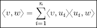
THEOREM 1.14.– Let (u1, . . . , un) be an orthonormal basis of (V, 〈, 〉), dim(V ) = n. Then, ∀v, w ∈ V :
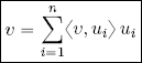
1) Decomposition theorem on an orthonormal basis:

2) Parseval’s identity7:
3) Plancherel’s theorem8:

Proof of 1: an immediate consequence of Theorem 1.12. Given that (u1, . . . , un) is a basis, v ∈ span(u1, . . . , un); furthermore, (u1, . . . , un) is orthonormal, so ![]() . It is not necessary to divide by ‖ui‖2 when summing since ‖ui‖ = 1 ∀i.
. It is not necessary to divide by ‖ui‖2 when summing since ‖ui‖ = 1 ∀i.
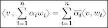
Proof of 2: using point 1 it is possible to write ![]() , and calculating the inner product of v, written in this way, and w, using equation [1.1], we obtain:
, and calculating the inner product of v, written in this way, and w, using equation [1.1], we obtain:
Proof of 3: writing w = v on the left-hand side of Parseval’s identity gives us 〈v, v〉 = ‖v‖2. On the right-hand side, we have:
hence ![]() .
.
NOTE.–
1) The physical interpretation of Plancherel’s theorem is as follows: the energy of v, measured as the square of the norm, can be decomposed using the sum of the squared moduli of each projection of v on the n directions of the orthonormal basis (u1, ..., un).
In Fourier theory, the directions of the orthonormal basis are fundamental harmonics (sines and cosines with defined frequencies): this is why Fourier analysis may be referred to as harmonic analysis.
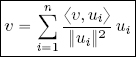
2) If (u1, . . . , un) is an orthogonal, rather than an orthonormal, basis, then using the projector formula and theorem 1.12, the results of Theorem 1.14 can be written as:
a) decomposition of v ∈ V on an orthogonal basis:
b) Parseval’s identity for an orthogonal basis:
c) Plancherel’s theorem for an orthogonal basis:
The following exercise is designed to test the reader’s knowledge of the theory of finite-dimensional inner product spaces. The two subsequent exercises explicitly include inner products which are non-Euclidean.
Exercise 1.1
Consider the complex Euclidean inner product space ![]() 3 and the following three vectors:
3 and the following three vectors:
1) Determine the orthogonality relationships between vectors u, v, w.
2) Calculate the norm of u, v, w and the Euclidean distances between them.
3) Verify that (u, v, w) is a (non-orthogonal) basis of ![]() 3.
3.
4) Let S be the vector subspace of ![]() 3 generated by u and w. Calculate PSv, the orthogonal projection of v onto S. Calculate d(v, PSv), that is, the Euclidean distance between v and its projection onto S, and verify that this minimizes the distance between v and the vectors of S (hint: look at the square of the distance).
3 generated by u and w. Calculate PSv, the orthogonal projection of v onto S. Calculate d(v, PSv), that is, the Euclidean distance between v and its projection onto S, and verify that this minimizes the distance between v and the vectors of S (hint: look at the square of the distance).
5) Using the results of the previous questions, determine an orthogonal basis and an orthonormal basis for ![]() 3 without using the Gram-Schmidt orthonormalization process (hint: remember the geometric relationship between the residual vector r and the subspace S).
3 without using the Gram-Schmidt orthonormalization process (hint: remember the geometric relationship between the residual vector r and the subspace S).
6) Given a vector a = (2i, −1, 0), write the decomposition of a and Plancherel’s theorem in relation to the orthonormal basis identified in point 5. Use these results to identify the vector from the orthonormal basis which has the heaviest weight in the decomposition of a (and which gives the best “rough approximation” of a). Use a graphics program to draw the progressive vector sum of a, beginning with the rough approximation and adding finer details supplied by the other vectors.
Solution to Exercise 1.1
1) Evidently, ![]() , so by directly calculating the inner products: 〈u, v〉 = −2, 〈u, w〉 = 0 et
, so by directly calculating the inner products: 〈u, v〉 = −2, 〈u, w〉 = 0 et ![]() .
.
2) By direct calculation: ![]() . After calculating the difference vectors, we obtain:
. After calculating the difference vectors, we obtain: ![]() ,
, ![]() .
.
3) The three vectors u, v, w are linearly independent, so they form a basis in ![]() 3. This basis is not orthogonal since only vectors u and w are orthogonal.
3. This basis is not orthogonal since only vectors u and w are orthogonal.
4) S = span(u, w). Since (u, w) is an orthogonal basis in S, we can write:
The residual vector of the projection of v on S is r = v − PSv = (2i, 0, 0) and thus d(v, PSv)2 = ‖r‖2 = 4. The most general vector in S is ![]() and
and ![]() . This confirms that PSv is the vector in S with the minimum distance from v in relation to the Euclidean norm.
. This confirms that PSv is the vector in S with the minimum distance from v in relation to the Euclidean norm.
5) r is orthogonal to S, which is generated by u and w, hence (u, w, r) is a set of orthogonal vectors in ![]() 3, that is, an orthogonal basis of
3, that is, an orthogonal basis of ![]() 3. To obtain an orthonormal basis, we then simply divide each vector by its norm:
3. To obtain an orthonormal basis, we then simply divide each vector by its norm:
6) Decomposition: ![]() .
.
Plancherel’s theorem: ![]() .
.
The vector with the heaviest weight in the reconstruction of a is thus r̂: this vector gives the best rough approximation of a. By calculating the vector sum of this rough representation and the other two vectors, we can reconstruct the “fine details” of a, first with ŵ and then with û.
Exercise 1.2
Let M(n, ![]() ) be the space of n × n complex matrices. The application ϕ : M(n,
) be the space of n × n complex matrices. The application ϕ : M(n, ![]() ) × M(n,
) × M(n, ![]() ) →
) → ![]() is defined by:
is defined by:
where ![]() denotes the adjoint matrix of B and tr is the matrix trace. Prove that ϕ is an inner product.
denotes the adjoint matrix of B and tr is the matrix trace. Prove that ϕ is an inner product.
Solution to Exercise 1.2
The distributive property of matrix multiplication for addition and the linearity of the trace establishes the linearity of ϕ in relation to the first variable.
Now, let us prove that ϕ is Hermitian. Let A = (ai,j)1≼i,j≼n and B = (bi,j)1≼i,j≼n be two matrices in M(n, ![]() ). Let
). Let ![]() be the coefficients of the matrix B† and let
be the coefficients of the matrix B† and let ![]() be the coefficients of A†.
be the coefficients of A†.
This gives us:
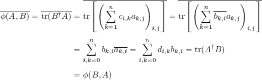
Thus, ϕ is a sesquilinear Hermitian form. Furthermore, ϕ is positive:
It is also definite:

Thus, ϕ is an inner product.
Exercise 1.3
Let E = ℝ[X] be the vector space of single variable polynomials with real coefficients. For P, Q ∈ E, take:
1) Remember that ![]() means that Ǝ a, C > 0 such that |t − t0| < a
means that Ǝ a, C > 0 such that |t − t0| < a ![]() |f(t)| ≼ C |g(t)|. Prove that for all P, Q ∈ E, this is equal to:
|f(t)| ≼ C |g(t)|. Prove that for all P, Q ∈ E, this is equal to:
and:
Use this result to deduce that Φ is definite over E × E.
2) Prove that Φ is an inner product over E, which we shall note 〈 , 〉.
3) For n ∈ ℕ, let Tn be the n-th Chebyshev polynomial, that is, the only polynomial such that ∀θ ∈ ℝ, Tn(cos θ) = cos(nθ). Applying the substitution t = cos θ, show that (Tn)n∈ℕ is an orthogonal family in E. Hint: use the trigonometric formula [1.13]:
4) Prove that for all n ∈ ℕ, (T0, . . . , Tn) is an orthogonal basis of ℝn[X], the vector space of polynomials in ℝ[X] of degree less than or equal to n. Deduce that (Tn)n∈ℕ is an orthogonal basis in the algebraic sense: every element in E is a finite linear combination of elements in the basis of E.
5) Calculate the norm of Tn for all n and deduce an orthonormal basis (in the algebraic sense) of E using this result.
Solution to Exercise 1.3
1) We write ![]() . Since P and Q are polynomials, the function
. Since P and Q are polynomials, the function ![]() is continuous in a neighborhood V1(1) and thus, according to the Weierstrass theorem, it is bounded in this neighborhood, that is, Ǝ C1 > 0 such that
is continuous in a neighborhood V1(1) and thus, according to the Weierstrass theorem, it is bounded in this neighborhood, that is, Ǝ C1 > 0 such that ![]() . Similarly, the function
. Similarly, the function ![]() is continuous in a neighborhood V2(−1), thus Ǝ C2 > 0 such that
is continuous in a neighborhood V2(−1), thus Ǝ C2 > 0 such that ![]() . This gives us:
. This gives us:
and:
This implies that the integral defining Φ is definite; f(t) is continuous over (−1, 1) and therefore can be integrated. The result which we have just proved shows that f(t) is integrable in a right neighborhood of –1 and a left neighborhood of 1, as the integral of its absolute value is incremented by an integrable function in both cases.
2) The bilinearity of Φ is obtained from the linearity of the integral using direct calculation. Its symmetry is a consequence of that of the dot product between functions. The only property which is not immediately evident is definite positiveness. Let us start by proving positiveness:
and9:
but the only polynomial with an infinite number of roots is the null polynomial 0(t) ≡ 0, so P = 0. Φ is therefore an inner product on E.
3) For all n, m ∈ ℕ:

So, for all n ≠ m, we have:
that is, Chebyshev polynomials form an orthogonal family of polynomials in relation to the inner product defined above.
4) The family (T0, T1, . . . , Tn) is an orthogonal (and thus free) of n+1 elements of ℝ[X], which is of dimension n + 1, meaning that it is an orthogonal basis of ℝn[X]. To show that (Tn)n∈ℕ is a basis in the algebraic sense of E, consider a polynomial P ∈ E of an arbitrary degree d ∈ ℕ, i.e. P ∈ ℝd[X], and note that (T0, T1, . . . , Td) is an orthogonal (free) family of generators of ℝd[X], that is, a basis in the algebraic sense of the term.
5) The norm of Tn is calculated using the following equality:
which was demonstrated in point 3. Taking n = m, we have:

hence ![]() . Finally, the family:
. Finally, the family:

is an orthonormal basis of the vector space of first-order polynomials with real coefficients E□
1.9. Summary
In this chapter, we have examined the properties of real and complex inner products, highlighting their differences. We noted that the symmetrical and bilinear properties of the real inner product must be replaced by conjugate symmetry and sesquilinearity in order to obtain a set of properties which are compatible with definite positivity. This final property is essential in order to produce a norm from a scalar product.
We noted that the prototype for all inner product spaces, or pre-Hilbert spaces, of finite dimension n is the Euclidean space ![]() n, where
n, where ![]() = ℝ or
= ℝ or ![]() =
= ![]() .
.
Using the inner product, the concept of orthogonality between vectors can be extended to any inner product space. Two vectors are orthogonal if their inner product is null. The null vector is the only vector which is orthogonal to all other vectors, and the property of definite positiveness means that it is the only vector to be orthogonal to itself. If two vectors have the same inner product with all other vectors, that is, the same projection in every direction, then these vectors coincide.
A norm on a vector space is said to be a Hilbert norm if an inner product can be defined which generates the norm in a canonical manner. Remarkably, a norm is a Hilbert norm if and only if it satisfies the parallelogram law; this holds true for both finite and infinite dimensions. The polarization law can be used to define an inner product which is compatible with a Hilbert norm.
Vector orthogonality implies linear independence, guaranteeing that a set of n orthogonal vectors in a vector space of dimension n will constitute a basis. The expansion of a vector on an orthonormal basis is trivial: the components in relation to this basis are the inner products of the vector with the basis vectors. It is therefore much simpler to calculate components in such cases because, if the basis is not orthonormal, then a linear system of equations must be solved.
The concept of orthogonal projection on a vector subspace S was also presented. Given an orthogonal basis of this space, the projection can be represented as an expansion over the vectors of the basis, with coefficients given by the inner products (which are normalized if the basis is not orthonormalized). We have seen that the difference between a vector and its orthogonal projection, known as the residual vector, is orthogonal to the projection subspace S. We also demonstrated that the orthogonal projection is the vector in S which minimizes the distance (in relation to the norm of the vector space) between the vector and the vectors of S.
Given an inner product space, of finite or infinite dimensions, an orthonormal basis can always be defined using the Gram-Schmidt orthonormalization algorithm.
Finally, we proved the important Parseval identity and Plancherel’s theorem in relation to an orthonormal or orthogonal basis. The extension of these properties to infinite dimensions is presented in Chapter 5.
- 1 i.e. is the abbreviation of the Latin expression “id est”, meaning “that is”. This term is often used in mathematical literature.
- 2 The symbols z* and
 represent the complex conjugation, i.e. if z ∈
  , z = a + ib, a, b ∈ ℝ, then z* = = a − ib. We recall that
  and z = if and only if ∈ ℝ.
 - 3 Sesqui comes from the Latin semisque, meaning one and a half times. This term is used to highlight the fact that there are not two instances of linearity, but one “and a half”, due to the presence of the complex conjugation.
- 4 For the French mathematician Charles Hermite (1822, Dieuze-1901, Paris).
- 5 Leopold Kronecker (1823, Liegnitz-1891, Berlin).
- 6 Jørgen Pedersen Gram (1850, Nustrup-1916, Copenhagen), Erhard Schmidt (1876, Tatu-1959, Berlin).
- 7 Marc-Antoine de Parseval des Chêsnes (1755, Rosières-aux-Salines-1836, Paris).
- 8 Michel Plancherel (1885, Bussy-1967, Zurich).
- 9 a.e.: almost everywhere (see Chapter 3).