2
The Discrete Fourier Transform and its Applications to Signal and Image Processing
The information presented in the previous chapter (Chapter 1) concerning complex inner product spaces and their properties lays the foundations for a very simple introduction to the discrete Fourier transform (DFT).
We simply need to prove that certain functions of complex exponentials constitute an orthogonal basis for a complex inner product space of finite dimension.
From a mathematical standpoint, the DFT is a simple change of basis in a vector space; however, its interpretation is of crucial importance and is extremely useful in the context of applications, notably in signal theory, as we shall see in section 2.6.
This section draws on the excellent work of M. Frazier (2001).
2.1. The space ℓ2(ℤN) and its canonical basis
In order to introduce the vector space in which the DFT is to be constructed, we need to make a few adjustments to the notation used thus far.
We shall continue to work with complex vectors with a number of components N, 1 < N < +∞, but a vector in ![]() N will be considered as a finite sequence.
N will be considered as a finite sequence.
Our first task is to define ℤN.
DEFINITION 2.1.– Two integers i, j ∈ ℤ are said to be congruent modulo N if their difference is divisible by N, that is:
meaning that we can write a = b + mN. The (Gaussian) notation for two integers which are congruent modulo N is:
Congruence modulo N can be shown to be an equivalence relationship in ℤ. Like all equivalence relationships, it creates a partition of ℤ into distinct equivalence classes. The set of these equivalence classes is written as:
A (finite) sequence of complex values on ℤN is a function:
In practice, circular or “clock” arithmetic is applied: this consists of identifying a sequence defined on ℤN as a sequence defined on {0, 1, . . . , N − 1} and extended to ℤ by N-periodicity:
that is, given the definition of z(j) when j ∈ {0, 1, . . . , N − 1}, in order to determine z(j) when j ∉ {0, . . . , N − 1}, we must add an integer multiple of N to j. This is written as mN, m ∈ ℤ such that ![]() = j + mN ∈ {0, 1, . . . , N − 1}. We then define z(j + mN) = z(
= j + mN ∈ {0, 1, . . . , N − 1}. We then define z(j + mN) = z(![]() ). An example is shown below.
). An example is shown below.
The value of m for which −21 + 12m falls within {0, . . . , 11} is m = 2, and in this case we have −21 + 2 · 12 = 3, which implies ![]() .
.
Despite the fact that ℤN is often considered to represent the set of canonical representatives {0, 1, . . . , N − 1}, we can, in fact, consider z to be defined over any sub-set of ℤ given by N consecutive integers, and not necessarily over {0, . . . , N − 1}. This convention will be used throughout this book.
The complex vector space that will be used in this section is the set of all sequences of complex values over ℤN:
The reason for using this particular notation will become clear later.
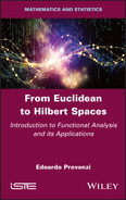
ℓ2(ℤN) is a complex vector space with the usual scalar summation and multiplication operators, that is, given z, w ∈ ℓ2(ℤN), α ∈ ![]() , the sum and multiplication by a complex vector are defined as follows:
, the sum and multiplication by a complex vector are defined as follows:
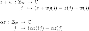
ℓ2(ℤN) is of dimension N: the application which associates each sequence z ∈ ℓ2(ℤN) with its images (z(0), z(1), . . . , z(N − 1)):
is a linear isomorphism (the proof is left to the reader). z will be represented as a row vector or as a column vector as the case requires.
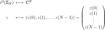
The isomorphism above allows us to define the canonical basis B of ℓ2(ℤN) as the set of the following N sequences:
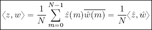
We can also introduce an inner product into ℓ2(ℤN) using:

so z, w ∈ ℓ2(ℤN) are orthogonal if and only if ![]() .
.
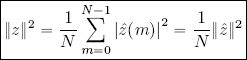
The norm induced by this inner product is:
which will be referred to as the ℓ2(ℤN) norm.
2.1.1. The orthogonal basis of complex exponentials in ℓ2(ℤN)
In this section, we are going to define the function system that will be essential to the development of the DFT.
First, we recall these basic facts:
- 1) for an arbitrary z ∈
 , z = ρ[cos α + i sin α] = ρeiα, ρ, α ∈ ℝ, ρ ≽ 0 ;
 - 2) Euler’s formulas:
 ;
; - 3) |z| = 1 ⇔ z = eiα;
- 4) eiα = ei(α+2πk), k ∈ ℤ;
- 5) as a specific instance of the previous point, if α = 0, we obtain:
- 6) eiαeiβ = ei(α+β);
- 7) (eiα)n = einα;
- 8)
 ;
; - 9) given z = ρeiα, the solutions to the equation wN = z are the N complex roots given by the equation:
 ;
; - 10) specifically:
roots N-ths of the unit : ![]() .
.
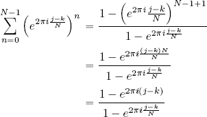
We also need to recall the geometric summation formula, defined by:

If z = 1, then Sk = k + 1. If z ≠ 1, we observe that:
hence:

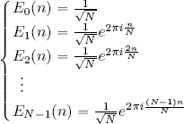
Now, consider the sequences in ℓ2(ℤN) defined by the following complex exponentials:
where:

Hence:
– ?0 is the constant sequence ?0(n) ≡ 1 ∀n ∈ ℤN;
– ?1 is the sequence ![]() ;
;
– ?2 is the sequence ![]() ;
;
– ?N−1 is the sequence ![]() .
.
The general sequence is:
where (ωm)n is the n-th power of the N-th roots of the unit, ∀n ∈ {0, ..., N − 1}, so:
From formula z = eiα = [cos α + i sin α], we know that the system defined above is a set of sequences of values which oscillate at different frequencies, since the arguments of the cos and sin functions change with the coefficients m and n. As we shall see, the signification of these frequencies is crucial to Fourier analysis.
For now, let us focus on proving that the exponential system defined above is an orthogonal basis of ℓ2(ℤN). This proof relies on a preliminary lemma.
LEMMA 2.1.– For all j, k ∈ {0, 1, . . . , N − 1}, we have:
The physical interpretation of this key formula will be discussed later. Before going further with the proof, note that in the case where j, k ∈ ℤN, j ≠ k, we have j − k ∈ {1, 2, . . . , N − 1}, so ![]() .
.
PROOF.– This proof covers the first summation, but it is evident that this demonstration also holds for the second summation. We start by using the properties of complex exponentials to rewrite the formula as follows:
Let us analyze the following two cases:
– if j = k, the exponentials in the sum are equal to 1, since ![]() , and thus:
, and thus:
– if j ≠ k, the exponentials are ≠ 1, so, using the geometric summation formula:
Since j – k = m ∈ ℤ, e2πi(j – k) = 1, the numerator of the final formula is 0 when j ≠ k. The denominator, on the other hand, never cancels out; as we saw in the remark before the proof, if j ≠ k, then ![]() . In this case, the summation is equal to 0. □
. In this case, the summation is equal to 0. □
The demonstration that ? is an orthogonal basis of ℓ2(ℤN) is now trivial.
THEOREM 2.1.– ? = (?0, . . . , ?N−1) is an orthogonal basis of ℓ2(ℤN).
PROOF.– ? is given by N elements of an N –dimensional inner product space, so if we can prove that ? is an orthogonal family, then the theorem is also proved. We know that an orthogonal family is free, and a free family of N vectors in an N–dimensional vector space is a basis.
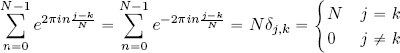
We thus calculate the inner products 〈?j, ?k〉, ∀j, k ∈ {0, . . . , N − 1}:
using Lemma 2.1 to give us the final equality, which proves that 〈?j, ?k〉 = Nδj,k, that is, the elements in the basis are mutually orthogonal.
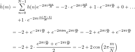
If we consider that j = k = m in equation 〈?j, ?k〉 = Nδj,k , then 〈?m, ?m〉 = Nδm,m = N hence:
Now, let us consider two examples in which the expression of the complex exponentials is particularly simple: N = 2 and N = 4 (the expression using N = 3 is not quite so simple):
1) N = 2. ℓ2(ℤ2) = {z = (z(0), z(1)) ∈ ![]() 2}, in this case
2}, in this case ![]() and thus:
and thus:

However, eπi = cos(π) + i sin(π) = −1, so ?1 = (1, −1). Thus:
is the basis of complex exponentials in ℓ2(ℤ2). Note the presence of a constant sequence (the first) and an oscillating sequence (the second). This particular feature of the basis will be discussed in greater detail later.
2) N = 4. ℓ2(ℤ4) = {z = (z(0), z(1), z(2), z(3)) ∈ ![]() 4}: the Fourier basis is obtained from four complex sequences, each with four components. Verification that the basis of complex exponentials of ℓ2(ℤ4) is:
4}: the Fourier basis is obtained from four complex sequences, each with four components. Verification that the basis of complex exponentials of ℓ2(ℤ4) is:
is left to the reader. Results [1.10], [1.11] and [1.12] from section 1.8 may be used to write the following formulas, which are valid for any two elements z, w ∈ ℓ2(ℤN):
– decomposition on the orthogonal basis ?:

– Parseval’s identity for the orthogonal basis ?:
– Plancherel’s theorem for ?:
The expressions above are calculated explicitly in section 2.3.
There are several ways of renormalizing the basis ?. Two of the most widespread approaches, which can also be used to define the DFT, are discussed in the next two sections.
2.2. The orthonormal Fourier basis of ℓ2(ℤN)
As we saw in section 2.1.1, the norm ℓ2(ℤN) of all sequences ?m is ![]() ; evidently, an orthonormal basis can therefore be obtained by dividing by
; evidently, an orthonormal basis can therefore be obtained by dividing by ![]() . This justifies Definition 2.2.
. This justifies Definition 2.2.
DEFINITION 2.2.– The orthonormal Fourier basis of ℓ2(ℤN) is the set:
of the N sequences Em ∈ ℓ2(ℤN):
where:
The general sequence of the orthonormal Fourier basis is:
and the orthonormality formula 〈Ej, Ek〉 = δj,k holds true.
Using formulas [2.2] and [2.3], we can say that:
is the orthonormal Fourier basis of ℓ2(ℤ2) and:
is the orthonormal Fourier basis of ℓ2(ℤ4).
The translation of theorem 1.14 for ℓ2(ℤN) equipped with the orthonormal Fourier basis is as follows. Given arbitrary elements z, w ∈ ℓ2(ℤN), we have:
– a decomposition on the orthonormal Fourier basis:
– Parseval’s identity:
– Plancherel’s theorem:
2.3. The orthogonal Fourier basis of ℓ2(ℤN)
Although the normalization constant ![]() , which appears in the definition of the orthonormal Fourier basis, might appear to be the most logical choice for normalizing the basis ? in ℓ2(ℤN), another normalization is more commonly used in practical applications. The reason for this choice, shown below, is that it simplifies the writing of several other formulas.
, which appears in the definition of the orthonormal Fourier basis, might appear to be the most logical choice for normalizing the basis ? in ℓ2(ℤN), another normalization is more commonly used in practical applications. The reason for this choice, shown below, is that it simplifies the writing of several other formulas.
DEFINITION 2.3.– The orthogonal Fourier basis of ℓ2(ℤN) is the set:
of N sequences Fm ∈ ℓ2(ℤN):
where:

The general sequence of the orthogonal Fourier basis is:
The relationships between the three bases ?, E and F are:
Using the formulas above, the orthogonal Fourier bases of ℓ2(ℤ2) and ℓ2(ℤ4) are easy to calculate:
– orthogonal Fourier basis of ℓ2(ℤ2):
– orthogonal Fourier basis of ℓ2(ℤ4) :
Again, using relationship [2.12], we can determine the equivalents of formulas [2.9] or [2.4], [2.10] or [2.5] and [2.11] or [2.6] for two arbitrary elements z, w ∈ ℓ2(ℤN):
– decomposition on the orthogonal Fourier basis:
– Parseval’s identity for the orthogonal Fourier basis:
– Plancherel’s theorem for the orthogonal Fourier basis:
Table 2.1 supplies a helpful summary of the differences between these bases and formulas:
Table 2.1. Different normalizations of Fourier bases and relative formulas
| Basis | Decomposition | Parseval’s identity | Plancherel ’s theorem |
|---|---|---|---|
| ? | |||
| E | |||
| F |
2.4. Fourier coefficients and the discrete Fourier transform
The definition of the DFT varies from author to author and from application to application. The two most widespread definitions use the orthonormal basis E and a blend of the orthogonal bases ? and F .
These two versions are useful for different reasons:
– using the orthonormal basis E allows us to obtain unitary operators;
– using a blend of the orthogonal bases ? and F makes it possible to simplify many formulas, including the convolution formula, widely used in applications, which will be discussed later.
For the purposes of this book, we shall use formulas obtained by a blend of the orthogonal bases ? and F. This decision was made for reasons of coherency with various mathematical programs, notably MATLAB.
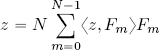
First, let us reconsider the following decomposition:
However, ?m/N = Fm, so:
that is, any given element z ∈ ℓ2(ℤN) can be decomposed over the orthogonal Fourier basis F with the components given by the inner products of z with elements of the basis ?.
Using the definition of the inner product of ℓ2(ℤN), we can write:
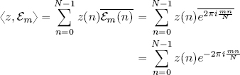
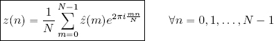
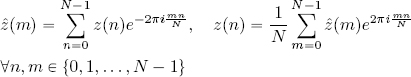
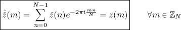
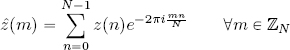
DEFINITION 2.4.– Given any z ∈ ℓ2(ℤN), the complex vectors 〈z, ?m〉, m ∈ {0, 1, . . . , N − 1} are known as the Fourier coefficients of z, noted ẑ(m). Explicitly:
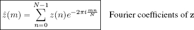
The sequence of Fourier coefficients of z is written using ẑ ∈ ℓ2(ℤN):
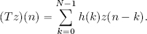
The linear operator which transforms z ∈ ℓ2(ℤN) into the sequence ẑ ∈ ℓ2(ℤN) of its Fourier coefficients, that is:
is known as the discrete Fourier transform, or DFT.
It is important to note that the variable of z is n, while the variable of ẑ is m. The interpretation of n and m in the context of signal theory will be given in section 2.6; for now, note simply that n is the discrete value of an instant in time (or a position in space) at which a signal z is measured, whereas m is proportional to the oscillation frequency of a wave (harmonic) and is a multiple of a fundamental frequency. The DFT is used to translate a description of a signal in terms of temporal (or spatial) samples into a description in terms of signal frequencies. This notion will be formalized in section 2.6.
Using the definitions given above, the decomposition of z may be written as follows:
that is, the Fourier coefficients of z are the components of z in the orthogonal Fourier basis F:
Using the notation introduced above, the theorem of decomposition on the orthonormal Fourier basis, Parseval’s identity and Plancherel’s theorem may be rewritten as:
– decomposition of z on the orthogonal Fourier basis:
– Parseval’s identity:
– Plancherel’s theorem :
2.4.1. The inverse discrete Fourier transform
It is interesting to compare formulas [2.15] and [2.19]:
The first relationship states that given the values of z(n), the values of ẑ(m) can be reconstructed using formula [2.15].
The second relationship states that given the values of ẑ(m), the values of z(n) can be reconstructed using formula [2.19].
There is thus a “duality” between the two formulas: it is possible to obtain sequence z from sequence ẑ and vice versa using relationships [2.15] and [2.19].
This duality is formalized in Definition 2.5 and Theorem 2.2.
DEFINITION 2.5.– The linear operator:
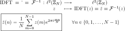
is known as the inverse discrete Fourier transform, or IDFT.
THEOREM 2.2.– The IDFT is the inverse linear operator of the DFT and vice versa:
or, in other terms,
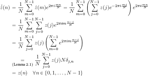
PROOF.– We wish to prove that the composition between the DFT and the IDFT and between the IDFT and the DFT gives the identity operator id: the DFT∘IDFT=IDFT∘DFT= id, id(z) = z, ∀z ∈ ℓ2(ℤN).
We start by verifying that, given an arbitrary sequence z ∈ ℓ2(ℤN) and applying the DFT to obtain the sequence of Fourier coefficients ẑ ∈ ℓ2(ℤN), it is possible to obtain the original sequence by applying the IDFT:
Before writing the composition, it is important to note that the summation index – the symbol of which is unimportant – should not be confused with the fixed variables n, m in ž(n) and ẑ(m). To avoid this problem we will use the neutral symbol j.
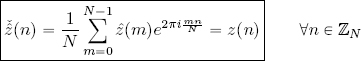
Now, let us verify that the inverse composition produces the same identity:

Thus, ![]() and
and ![]() which concludes our proof. □
which concludes our proof. □
Note the similarity between the DFT and the IDFT: the only differences are the coefficient 1/N and the sign of the complex exponential.
We wish to draw the reader’s attention to the formulas demonstrated above:
DEFINITION 2.6.– The pair (z, ẑ) ∈ ℓ2(ℤN) × ℓ2(ℤN) is known as a Fourier pair.
2.4.2. Definition of the DFT and the IDFT with the orthonormal Fourier basis
Box 2.1. Discrete orthonormal Fourier analysis
As we can see, the greatest advantage of using the orthonormal Fourier basis in defining the objects used in Fourier analysis is that the DFT and the IDFT are operators which conserve the inner product, and consequently the norm; they are therefore represented using unitary matrices.
We also see that, independently of the definition used, the product of the coefficients of ẑ and ž must always be equal to 1/N to guarantee that IDFT = DFT−1.
2.4.3. The real (orthonormal) Fourier basis
The Fourier basis and DFT can be written using real notation. The advantage of a real DFT is that, if z is real, we can avoid the need to introduce imaginary components. For simplicity’s sake, we shall focus on the orthonormal Fourier basis.
First, we must determine whether N is even or odd. Let us begin with the case where N is even: N = 2M, M ∈ ℕ, M ≽ 1. In this case, ∀n = 0, 1, . . . , N − 1, we write:
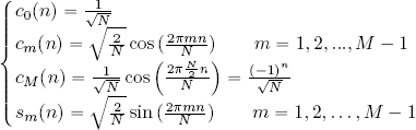
If N = 2M + 1 is odd, c0, cm and sm are defined in the same way as above, but m = N/2 should not be considered as in this case N/2 is not an integer.
THEOREM 2.3.– The set {c0, c1, . . . , cM−1, cM, s1, . . . , sM−1}, when N = 2M, or the set {c0, c1, . . . , cM−1, s1, . . . , sM−1}, when N = 2M +1, is an orthonormal basis of ℓ2(ℤN). Thus, for all z ∈ ℓ2(ℤN):
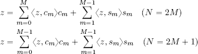
DEFINITION 2.7.– The real orthonormal Fourier basis of ℓ2(ℤN) is the set of sequences of ℓ2(ℤN) {c0, c1, . . . , cM−1, cM, s1, . . . , sM−1} when N = 2M, our the set of sequences of ℓ2(ℤN) {c0, c1, . . . , cM−1, s1, . . . , sM−1} when N = 2M + 1.
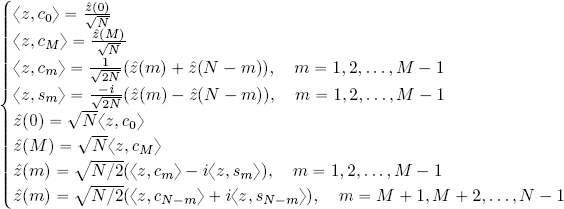
The relationship with the Fourier coefficients is obtained using the following formulas:
2.5. Matrix interpretation of the DFT and the IDFT
By definition, the DFT transforms sequences of ℓ2(ℤN) represented in the canonical basis B of ℓ2(ℤN) into sequences of ℓ2(ℤN) represented in the orthogonal Fourier basis F of ℓ2(ℤN) [2.17]:
The DFT is thus the operator used to operate the change from the canonical basis B of ℓ2(ℤN) to the Fourier basis F of ℓ2(ℤN), and, consequently, the IDFT is the opposite operator.
We wish to establish a matrix representation of these two linear operators DFT and IDFT. To do this, we shall use a notation which is widely used in literature concerning the DFT: ![]() . Using the properties of complex exponentials, we can write:
. Using the properties of complex exponentials, we can write:
and the Fourier coefficients can thus be written as:
We define the matrix WN containing the elements ![]() :
:
that is, explicitly:
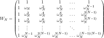
This N × N matrix is called Sylvester matrix1. It is symmetrical: ![]() , i.e. wmn = wnm (an obvious consequence of the definition of wmn , since
, i.e. wmn = wnm (an obvious consequence of the definition of wmn , since ![]() ) and each line or column is obtained by the geometric progression2 of a power of ωN. A matrix of this type is known as a Vandermonde matrix3.
) and each line or column is obtained by the geometric progression2 of a power of ωN. A matrix of this type is known as a Vandermonde matrix3.
By convention, when considering WN, we examine the variability of the indices of the lines and columns between 0 and N − 1 (in place of canonical variability, from 1 to N). This convention is the reason why all elements in the first line (m = 0) and all elements in the first column (n = 0) are equal to 1.
If we apply WN to z considered as a column vector in ![]() N, then, by the definition of matrix product, we obtain a vector WNz whose m-th component (WNz)(m)4 is given by:
N, then, by the definition of matrix product, we obtain a vector WNz whose m-th component (WNz)(m)4 is given by:
thus:
Using the same approach, we can verify that the IDFT is implemented via the conjugate matrix of WN normalized by the coefficient 1/N (transposition is not required as WN is symmetrical):
WN is the change of basis matrix used to go from B to F, and ![]() is the change of basis matrix used to go from F to B.
is the change of basis matrix used to go from F to B.
OBSERVATIONS.– Using the definition of the DFT corresponding to equation [2.22], that is using the orthonormal Fourier basis, the associated matrix becomes ![]() . This is a unitary matrix, and thus its inverse matrix is
. This is a unitary matrix, and thus its inverse matrix is ![]() .
.
Examples:
– N = 2 : ω2 = e−2πi/2 = e−iπ = cos(π) − i sin(π) = −1, thus:
hence:
– N = 4 : ω4 = e−2πi/4 = e−iπ/2 = cos(π/2) − i sin(π/2) = −i, thus:
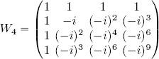
hence:

The inverse matrix is:

Note that the columns of matrix ![]() consist of the orthogonal basis F of ℓ2(ℤ4), as seen in formula [2.14]; this is coherent with the fact that this is the matrix used to change from the orthogonal basis F to the canonical basis of ℓ2(ℤ4).
consist of the orthogonal basis F of ℓ2(ℤ4), as seen in formula [2.14]; this is coherent with the fact that this is the matrix used to change from the orthogonal basis F to the canonical basis of ℓ2(ℤ4).
2.5.1. The fast Fourier transform
As we have seen, the action of the DFT on a signal z ∈ ℓ2(ℤN) can be represented as a matrix product.
We must therefore calculate N multiplications for each element ẑ(m) in the sequence ẑ ∈ ℓ2(ℤN). Since ẑ has N components, the complexity of the algorithm used to calculate the DFT is ![]() (N2).
(N2).
This complexity means that the DFT is extremely time-consuming when working with signals of large dimension. In practice, the Fourier transform was almost never used outside of a theoretical context (that is, in real-world applications) before the 1960s.
A breakthrough came in 1965, when Cooley and Tukey used symmetries concealed within the DFT to construct a fast algorithm for calculating the DFT: this algorithm is known as the fast Fourier transform (FFT).
The complexity of the FFT is of the order of ![]() (N log N), and, using modern computers, it allows the Fourier transform of large dimension signals to be calculated in under a second.
(N log N), and, using modern computers, it allows the Fourier transform of large dimension signals to be calculated in under a second.
The FFT is extremely efficient in cases where the signal dimension is a power of 2. This is the reason why a 512 or 1,024 format is typically used for digital images, enabling rapid and efficient processing using the FFT.
The development of the FFT is considered as one of the greatest scientific breakthroughs of the 20th century, as it enables the use of Fourier transforms in a vast array of practical applications.
2.6. The Fourier transform in signal processing
Fourier theory has applications in a wide range of domains, for example in solving ordinary and partial differential equations, classical and quantum physics, statistics and probabilities, and signal processing.
In this section, we shall highlight the crucial role of Fourier theory in signal processing in one dimension (1D).
2.6.1. Synthesis formula for 1D signals: decomposition on the harmonic basis
A discrete 1D signal of dimension N may be defined as the set of N samplings of a variable, which may be dependent on time, on a spatial dimension (x,y or z), or on another parameter with a single degree of freedom.
Two remarkable examples of discrete 1D signals, dependent on time or a single spatial dimension, are:
– the set of intensity values for a piece of music, sampled at N different moments in time;
– the set of grayscale values of a line or column in a simple image, corresponding to N different positions.
A discrete 1D signal can be processed using Fourier theory using the following basic identifications:
– the abstract mathematical representation of a discrete 1D signal is given by a sequence z ∈ ℓ2(ℤN);
– n ∈ ℤN = {0, 1, . . . , N − 1} represents the value of the parameter (time, spatial dimension, etc.) according to which the signal is sampled. The unit of measurement used for n is typically the second or meter;
– the energy of the signal z is associated with the square of the norm ‖z‖2.
The next step is to interpret the decomposition formula over the Fourier basis, the DFT and the IDFT, and Plancherel’s theorem in the context of signal processing.
The interpretation of Plancherel’s theorem in this case is simplest: the energy of the signal z is decomposed into the sum of the squared magnitudes of the Fourier coefficients.
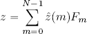
The decomposition formula over the Fourier basis, equation [2.19], is known as the synthesis formula in the context of signal processing:
Using this formula, the signal z can be reconstructed (or “synthesized") using the Fourier coefficients ẑ(m) and the oscillating functions ![]() .
.
The functions used in the signal synthesis operation are:
When m = 0, there is no oscillation; from m = 1 to m = N − 1 the functions ![]() oscillate at a certain frequency (m is therefore measured in hertz or rad/s). This will be discussed in detail in section 2.6.4. These functions are known as harmonics, a term derived from the field of music, as we see from Definition 2.8.
oscillate at a certain frequency (m is therefore measured in hertz or rad/s). This will be discussed in detail in section 2.6.4. These functions are known as harmonics, a term derived from the field of music, as we see from Definition 2.8.
DEFINITION 2.8 (harmonics).– The function ![]() is known as a fundamental (discrete) harmonic5 and the functions
is known as a fundamental (discrete) harmonic5 and the functions ![]() for m = 2, . . . , N − 1 are (discrete) harmonics of (higher) order m.
for m = 2, . . . , N − 1 are (discrete) harmonics of (higher) order m.
2.6.2. Signification of Fourier coefficients and spectrums of a 1D signal
The synthesis formula tells us that the signal z in the value n of its parameter can be reconstructed using a linear combination of harmonic waves of frequencies which are multiples of 1/N via the coefficient m: {0, 1/N, 2/N, . . . , (N −1)/N}. The complex scalars of the linear combination are the Fourier coefficients ẑ(m).
Each Fourier coefficient ẑ(m) ∈ ![]() may be written as:
may be written as:
where ![]() is the magnitude of the Fourier coefficient ẑ(m) and
is the magnitude of the Fourier coefficient ẑ(m) and ![]() is its argument.
is its argument.
Evidently, the “weight” which measures the importance of each harmonic ![]() in reconstructing a signal z is the magnitude6 of the Fourier coefficient ẑ(m):
in reconstructing a signal z is the magnitude6 of the Fourier coefficient ẑ(m):
|ẑ(m)| : measures the importance of the harmonic ![]() in reconstructing z. For this reason, in signal processing, the Fourier coefficient formula is known as the analysis formula:
in reconstructing z. For this reason, in signal processing, the Fourier coefficient formula is known as the analysis formula:
since ẑ allows us to analyze the frequency components of a signal.
If the discrete signal z is dependent on the time t (or a spatial dimension x), then the transformation z → ẑ obtained using the DFT enables us to go from a temporal (or spatial) representation of the signal to a frequential representation, or the Fourier space.
The Fourier transform is often defined as the equivalent of Newton’s prism for mathematics. Newton’s prism breaks down light into “hidden” frequency components corresponding to the colors of the spectrum. The Fourier transform reveals the frequency components which are “hidden” in any signal.
This analogy explain the terms used in Definition 2.9.
DEFINITION 2.9.– Given z ∈ ℓ2(ℤN):
– {|ẑ(m)|, m ∈ ℤN} is known as the amplitude spectrum of z, or simply the spectrum of z;
– {|ẑ(m)|2, m ∈ ℤN} is the power spectrum of z;
– {Arg(ẑ(m)), m ∈ ℤN} is the phase spectrum of z.
The signification of these spectra will be discussed in detail later.
Note the presence of one particularly special Fourier coefficient, ẑ(0), which provides information concerning the average value of z:
Where ![]() is the average value of the signal z.
is the average value of the signal z.
Introducing this expression of ẑ(0) into the synthesis formula and separating the first term from the rest of the sum, we obtain:
that is : 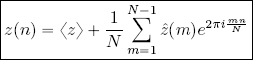
The Fourier coefficient ẑ(0) is known as the “DC” component of the synthesis formula, while the other terms constitute the “AC” component. This terminology is taken from the field of electronics, with DC standing for “direct current” (current of frequency zero) and AC standing for “alternating current”.
One way of interpreting the formula set out above is to say that z is decomposed into the sum of its mean value and the finer details reconstructed by higher order harmonics, weighted by the Fourier coefficients of z.
2.6.3. The synthesis formula and Fourier coefficients of the unit pulse
It is helpful to compare the synthesis formula with formula [2.1], that is:

Rewriting j−k = m ∈ ℤN, switching m and n (an acceptable substitution, as both are arbitrary values of ℤN) and normalizing by N, we obtain the following formula:

δ is known as the unit pulse. If we select the option “+” in the formula shown above, we obtain the synthesis formula for the unit pulse, in which all Fourier coefficients are unitary:
This result is particularly informative: the DFT transforms a signal which is completely “localized” at a value on its parameter into a signal which is fully “delocalized” across the spectrum: the harmonics for all frequencies have the same weight when reconstructing the signal.
Let us now calculate the Fourier coefficients of the constant signal , ![]() , we obtain:
, we obtain:

We see that the DFT of a constant signal (which is completely delocalized in relation to its parameter) is therefore a unit pulse in the Fourier domain, meaning that it is completely localized in its frequencies.
The generalization of this behavior for spaces which are more complicated than ℓ2(ℤN) – notably L2(Ω), Ω ⊆ ℝn, which we will examine later – forms the basis for understanding the Heisenberg uncertainty principle, the conceptual core of quantum mechanics.
Thanks to the results that we have discussed above, we can give a physical interpretation of the formula [2.1] in Lemma 2.1: the superposition of harmonic functions with frequencies which are integer multiples of one another is subjected to a destructive interference everywhere, except at one value where the harmonics experience a constructive interference.
Moreover, according to the synthesis formula, harmonics must be weighted differently in order to reconstruct any signal which is not a pulse.
2.6.4. High and low frequencies in the synthesis formula
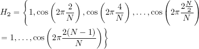
Let us take a closer look at the meaning of the frequency coefficients m in the set
which represents the value of the harmonics in each of the N parameters n.
For the sake of simplicity, we shall only consider the real part of the elements of the set above, that is
our remarks concerning the cosine are equally applicable to the sine.
Consider the behavior of cos ![]() when the value of m is between 0 and N −1, where N is even (the case where N is odd will be discussed later):
when the value of m is between 0 and N −1, where N is even (the case where N is odd will be discussed later):
– m = 0 : As we have already seen, in this case, there is no oscillation, but simply a series of constant values, ![]() , so:
, so:
– m = 1 :
The values of H1 represent N samples of a cosine oscillation. The cycle does not terminate as we do not consider the value n = N, which would give us ![]() . Figure 2.1 shows the graph of Hm for m = 1, N = 16;
. Figure 2.1 shows the graph of Hm for m = 1, N = 16;
– m = 2 :
The values of H2 represent N samples of two cosine oscillations. n = N/2 marks the end of a cosine cycle. Figure 2.2 shows the graph of Hm for m = 2, N = 16. We see that, for n = 8 = 16/2, the cosine value is 1.
Increasing m up to N/2, the oscillation frequency of the cosine increases. The maximum frequency is reached when m = N/2; in this case, ![]() , thus:
, thus:
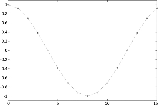
Figure 2.1. Hm for m = 1, N = 16
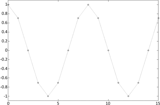
Figure 2.2. Hm for m = 2, N = 16
We might expect the cosine oscillation frequency to increase up to N − 1, but this is not the case. In reality, from m = N/2 + 1, the cosine oscillation frequency decreases. To understand this behavior, consider ![]() when m belongs to the
when m belongs to the ![]() , and apply the following change of variable:
, and apply the following change of variable:
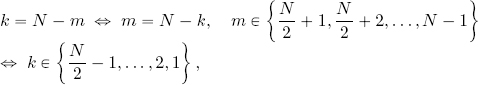
then, when m increases from ![]() up to N − 1, k decreases from
up to N − 1, k decreases from ![]() down to 1. Applying this variable change to the cosine, we obtain:
down to 1. Applying this variable change to the cosine, we obtain:
having used the periodicity and parity of the cosine.
Consequently:
Thus, the maximum number of harmonic oscillations is obtained when m = N/2, and is symmetrical about this value. For example, the graph of Hm for m = 9, N = 16 is exactly equal to the graph of Hm with m = 7, N = 16. Similarly, the graph of m = 15, N = 16 is exactly equal to the graph in Figure 2.1, representing Hm with m = 1, N = 16;
– evidently, if N is odd, the considerations set out above are valid for ![]() , the integer part of
, the integer part of ![]() , that is the integer closest to, but not greater than
, that is the integer closest to, but not greater than ![]() .
.
The elements described above are the reasons for certain choices of terminology:
– high frequencies: values of m close to ![]() ;
;
– low frequencies: values of m close to 0 or N − 1.
If the synthesis formula for a discrete signal z ∈ ℓ2(ℤN) includes Fourier coefficients ẑ(m) with a high magnitude for values of m which are close to N/2, the signal will be characterized by relatively violent variations (as in the case of high sounds, such as those produced by cymbals). However, if the Fourier coefficients with the highest modulus correspond to values of m close to 0 and N − 1, the signal will be characterized by “gentler” variations (as in the case of low sounds, such as those produced by bass drums).
The frequency m = N/2 is known as the Nyquist frequency7. This is the highest harmonic frequency which can appear in the synthesis formula for N samples of a signal.
2.6.5. Signal filtering in frequency representation
The DFT can be used to easily modify the frequency content of a signal, for example increasing the strength of the lowest or highest frequencies.
The standard approach is to obtain the Fourier space using the DFT then adjust the Fourier coefficients as required using a filter f : ℓ2(ℤN) → ℓ2(ℤN), which may be either a linear or a nonlinear transform. Finally, the IDFT is applied to the sequence of modified Fourier coefficients to reconstruct the original signal in its modified form.
The signal processing approach used in the frequency domain is shown in Figure 2.3.
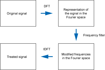
Figure 2.3. Filtering approach in the Fourier domain
Note that, in the IDFT ∘ f ∘ DFT transform composition, only f has the capacity to change the energy of the signal: the composition of the Fourier transform with its inverse produces an identity, so the energy of the original signal is retained.
One particularly important example of a filter f, defined in section 2.6.6, can be used to define the concept of the Fourier multiplier, defined in section 2.6.7.
2.6.6. The multiplication operator and its diagonal matrix representation
Let w : ℤN → ![]() be a fixed sequence in ℓ2(ℤN).
be a fixed sequence in ℓ2(ℤN).
DEFINITION 2.10.– The linear application below is known as the multiplication operator by sequence w:
where Mw(z) = w · z : ℤN → ![]() is the sequence defined by the point-wise (also called Hadamard) product of w and z:
is the sequence defined by the point-wise (also called Hadamard) product of w and z:
Note that if z is represented as a column vector in the canonical basis of ℓ2(ℤN), then the matrix associated with the operator Mw in relation to the canonical basis of ℓ2(ℤN) is a diagonal matrix Dw with diagonal elements given by the components of sequence w:

This provides the foundation for introducing the Fourier multiplier operator.
2.6.7. The Fourier multiplier operator
The Fourier multiplier operator – or multiplier – is one notable example of a frequency filter.
DEFINITION 2.11.– Given a sequence w : ℤN → ![]() , the Fourier multiplier by sequence w is the following operator:
, the Fourier multiplier by sequence w is the following operator:
that is, T(w) is the operator given by the composition
that is,
Applying the DFT to both sides of the definition of T(w), we see that the action of the Fourier multiplier is diagonal in the Fourier basis F:
Thus, T(w) multiplies the Fourier coefficients of z by the components of sequence w (making this operator a multiplier). This means that we can:
- – attenuate the low frequencies of a signal z by selecting a sequence w(m) with a low value of |w(m)| when m ≃ 0 and m ≃ N − 1;
- – attenuate the high frequencies of a signal z by selecting a sequence w(m) with a low value of |w(m)| when m ≃ N/2;
- – amplify the low frequencies of a signal z by selecting a sequence w(m) with a high value of |w(m)| when m ≃ 0 and m ≃ N − 1;
- – amplify the high frequencies of a signal z by selecting a sequence w(m) with a high value of |w(m)| when m ≃ N/2.
This information is used in graphic equalizers, used by musicians to adjust the level of high frequencies and bass notes in an audio signal.
2.7. Properties of the DFT
In this section, we shall demonstrate the most important properties of the DFT. We shall begin by recalling the translation property of a summation index:

This property will be used on several occasions, along with the following lemma.
LEMMA 2.2.– Let f : ℤ → ![]() be an N-periodic function, with N ∈ ℕ:
be an N-periodic function, with N ∈ ℕ:
Then, for all m ∈ ℤ :
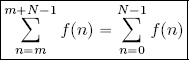
that is, the sum of an N-periodic function across any interval of size N is constant.
PROOF.– If m = 0, there is nothing to prove, so we may take m ∈ ℤ, m ≠ 0. Considering values of m > 0:

but, using [2.28]:
because of the N-periodicity of f, thus:
A similar demonstration may be used for cases where m < 0.
2.7.1. Periodicity of ẑ and ž
In what follows, we shall examine the most important properties of the discrete Fourier theory, starting with the periodicity of ẑ and ž.
By direct calculation, if a ∈ ℤ, then:
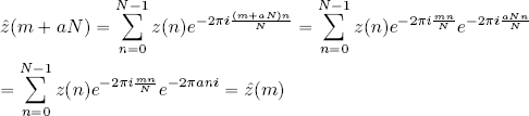
since e−2πani = cos(2πan)−i sin(2πan) = 1. The same calculation is used to prove ž(n + aN) = ž(n) ∀a ∈ ℤ.
Thanks to this property, the definitions of ẑ and ž can be extended to ℤ by considering the two N-periodic sequences:
and:
with a ∈ ℤ such that m + aN ∈ ℤN, or n + aN ∈ ℤN, respectively.
2.7.2. DFT and shift
We now wish to consider how the DFT of a signal z ∈ ℓ2(ℤN) varies in response to a shift in z by a quantity different to N. Another operator for ℓ2(ℤN) must be introduced in order to formalize this consideration.
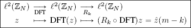
DEFINITION 2.12.– Take z ∈ ℓ2(ℤN). The following linear application is the right shift operator of the quantity k:
where Rk(z) : ℤN → ![]() is the sequence defined by the formula:
is the sequence defined by the formula:
The final two elements “turn” into the first two positions, as though following a circle. For this reason, Rk is also known as a circular shift operator or rotation operator.
Now, consider the composition of this shift operator with the DFT and, inversely, that of the DFT with the shift operator. We shall begin with this latter composition: DFT(z(n − k)), that is:

Theorem 2.4 shows that, due to the DFT, the action of the operator Rk is transformed into a multiplication by a complex exponential.
THEOREM 2.4.– Take z ∈ ℓ2(ℤN) and k ∈ ℤ. Then:
that is, if we define the sequence ![]() , then:
, then:
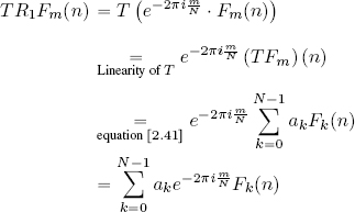
PROOF.–
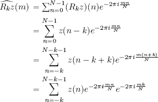
Factor ![]() is independent of the index n and can thus be left out of the summation:
is independent of the index n and can thus be left out of the summation:
Lemma 2.2 can be applied in this case as, by hypothesis, z is N-periodic and the exponential ![]() is itself an N-periodic function. □
is itself an N-periodic function. □
Note that, if we write ẑ(m) = |ẑ(m)| eiArg(ẑ(m)) then, since ![]() , product
, product ![]() only changes the phase of ẑ(m). This is the reason why we say that the DFT transforms the shift into a phase shift. The fact that the phase of the Fourier coefficients is modified by translations implies that the phase spectrum contains information regarding the geometry of the original signal.
only changes the phase of ẑ(m). This is the reason why we say that the DFT transforms the shift into a phase shift. The fact that the phase of the Fourier coefficients is modified by translations implies that the phase spectrum contains information regarding the geometry of the original signal.
2.7.2.1. Shift invariance of the spectrum
Theorem 2.4 highlights an important limitation of the Fourier transform. Since:
the magnitudes of the Fourier coefficients of z and of all its shifts are equal. Consequently, the magnitude of the Fourier coefficients |ẑ(m)| informs us of the (global) importance of the harmonic of frequency m in the reconstruction of the signal z, but not of its (local) position within the signal.
To gain a clearer understanding of this behavior, let us consider the unit pulse, to which an arbitrary shift is applied: Rkδ0. The spectrum of this signal is ![]() , but, as we have seen,
, but, as we have seen, ![]() for all m ∈ ℤN, thus
for all m ∈ ℤN, thus ![]() . The difference between this case and that of the non-shifted unit pulse is that, in the latter case, the spectrum is real and thus
. The difference between this case and that of the non-shifted unit pulse is that, in the latter case, the spectrum is real and thus ![]() .
.
The spectrum of the unit pulse is therefore exactly the same as that of any of its shifted forms. Knowledge of the spectrum alone is not sufficient to reconstruct the spatial location of a signal; to do this, we need information from the phase, which is not easy to interpret or handle.
One solution to this problem lies in using two transforms which “localize” the Fourier transform: the Gabor transform and the wavelet transform. These transforms lie outside the scope of this book, the interested reader can consult, for instance, Frazier (2001).
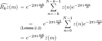
Now, let us analyze the composition of the shift operator and the DFT : ẑ(m − k), that is:
THEOREM 2.5.– Using the hypotheses from Theorem 2.4, this is equivalent to the formula:
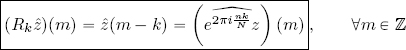
that is:
PROOF.–

The properties analyzed above may be summarized in the form of Fourier pairs, shown in Table 2.2. This information shows that the shift operation in the original representation of z becomes a phase change in the Fourier space; conversely, the shift operation in the Fourier space corresponds to a phase change (with a conjugate phase) in the original representation of z.
The following situation illustrates a particularly remarkable case. If N is an even value and k = N/2, then:
and:
so:
Thus, multiplying sequence z by (−1)n corresponds to shifting the spectrum by N/2. This operation is often used to center a spectrum on m = 0.
Table 2.2. Fourier pairs and translation
| Original representation | Fourier space |
|---|---|
| z(n − k) | |
| ẑ(m − k) |
Finally, note the relation between formula [2.30] and the diagonal representation of the operator Rk. Composing the left and right members of formula [2.30] with the IDFT, we obtain:
Using Ak and ![]() (diagonal, see section 2.6.6) to write the matrices associated with the operator Rk and with
(diagonal, see section 2.6.6) to write the matrices associated with the operator Rk and with ![]() in relation to the canonical basis, the previous equation can be rewritten as:
in relation to the canonical basis, the previous equation can be rewritten as:
This tells us that the matrix Ak associated with the shift operator Rk is similar to the diagonal matrix ![]() .
.
The invertible matrix which produces the matrix conjugation of Ak and ![]() is the Sylvester matrix WN, so we can say that the action of the shift operator Rk is diagonal in the Fourier space.
is the Sylvester matrix WN, so we can say that the action of the shift operator Rk is diagonal in the Fourier space.
2.7.3. DFT and conjugation
Given a sequence z ∈ ℓ2(ZN), the conjugate sequence z̅ is written as z̅ = (z̅(0), z̅(1), . . . , z̅(N − 1)), that is, ![]() .
.
The relationship between the DFT and conjugation is shown in Theorem 2.6.
THEOREM 2.6.– For all z ∈ ℓ2(ZN):
PROOF.–

COROLLARY 2.1.– z ∈ ℓ2(ℤN) is real, that is, z(n) ∈ ℝ ∀n ∈ ℤN, if and only if:
![]()
ẑ ∈ ℓ2(ℤN) is real, that is, ẑ(m) ∈ ℝ ∀m ∈ ℤN, if and only if:
PROOF.– As the DFT is an isomorphism of ℓ2(ℤN), z is real, that is, z = z̅, if and only if ![]() but, from Theorem 2.6, this also holds true when
but, from Theorem 2.6, this also holds true when ![]() .
.
ẑ is real if and only if ![]() , but the previous theorem states that
, but the previous theorem states that ![]() , implying that
, implying that ![]() , by simple substitution of the variable m ↔ −m. Hence:
, by simple substitution of the variable m ↔ −m. Hence:
Therefore ẑ is real ![]() . □
. □
Corollary 2.2 is an immediate consequence of the previous result.
COROLLARY 2.2.– z, ẑ ∈ ℓ2(ℤN) are simultaneously real if and only if they are symmetrical about 0, that is, z(n) = z(−n) and ẑ(m) = ẑ(−m), ∀m, n ∈ ℤN.
2.7.4. DFT and convolution
One of the most important properties of the Fourier transform relates to the convolution operation.
To understand this operation, we first note the formula for polynomial products.
If ![]() and
and ![]() , then:
, then:
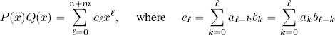
DEFINITION 2.13.– Take z, w ∈ ℓ2(ℤN). The convolution of z with w, written as z*w, is the sequence of ℓ2(ℤN) with components defined by:
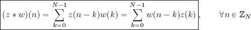
Convolution is symmetrical, that is z * w = w * z, due to the commutative nature of the product in ![]() .
.
The interaction between the DFT and convolution has a particularly elegant and useful property, described in Theorem 2.7.
THEOREM 2.7.– Take z, w ∈ ℓ2(ℤN). Then:

In other words, the Fourier transform of the convolution of z and w is the pointwise product of the Fourier transforms and vice versa: the inverse Fourier transform of the convolution of ẑ and ŵ is N times the pointwise product of z and w. In other words, we obtain the Fourier pairs shown in Table 2.3.
Table 2.3. Fourier pairs relative to convolution
| Original representation | Fourier space |
|---|---|
| z * w | ẑ · ŵ |
| Nz · w | ẑ * ŵ |
PROOF.– By definition :

The exponential is rewritten as:
Then:

Lemma 2.2 can be applied here as it is valid for any k ∈ ℤ. Thus:
The proof that the IDFT(ẑ * ŵ)(n) = z(n) · w(n) is very similar, by definition :
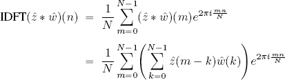
The exponential is rewritten as:
Then:
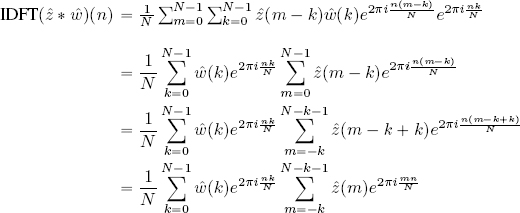
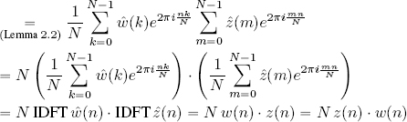
OBSERVATIONS.–
– In this proof, ![]() cannot be replaced with ŵ(m) before the final step, as the index k is still present in the second sum. ŵ(m) can only be substituted in once k has been eliminated.
cannot be replaced with ŵ(m) before the final step, as the index k is still present in the second sum. ŵ(m) can only be substituted in once k has been eliminated.
– Formulas [2.36] demonstrate a sort of “distributive property” in connection with convolution and the pointwise product: when the DFT is applied to a convolution product, it is distributed over the factors, and the convolution becomes a pointwise product. Inversely, when the IDFT is applied to a pointwise product, it is distributed over the factors, and the pointwise product becomes a convolution. Thus:
– Using the Fourier transform, a complex operation such as convolution can be transformed into a simple product of Fourier transforms (which can be calculated rapidly using the FFT). This result is particularly useful for signal processing applications. If we define the DFT using the normalization induced by the orthonormal Fourier basis, coefficients appear in the DFT formula of the convolution. These coefficients may be extremely large, particularly when dealing with DFTs in dimensions greater than 1 and/or large signals; this may result in calculation errors. The simplicity of formula [2.36] is the reason why many authors – and programmers – prefer the definition of Fourier coefficients used in this book to other definitions.
– Convolution is often carried out between a signal z and another signal w which is non-zero only on a support of size T. The value of T is important in choosing whether to apply the convolution operation directly or to use the FFT. The complexity of the direct convolution operation is ![]() (NT ); using the FFT, the complexity is
(NT ); using the FFT, the complexity is ![]() (N log N). It is therefore helpful to transform the convolution into a pointwise product with FFT in cases where T > log(N). For example, taking z ∈ ℓ2(ℤN) with N = 1, 000, then log(N) ≃ 7 and it is thus preferable to carry out the convolution z * w in the Fourier domain for all cases where the support of w is larger than 7.
(N log N). It is therefore helpful to transform the convolution into a pointwise product with FFT in cases where T > log(N). For example, taking z ∈ ℓ2(ℤN) with N = 1, 000, then log(N) ≃ 7 and it is thus preferable to carry out the convolution z * w in the Fourier domain for all cases where the support of w is larger than 7.
If one of the vectors in the convolution is fixed, we can define an endomorphism of ℓ2(ℤN).
DEFINITION 2.14.– Taking a fixed sequence w ∈ ℓ2(ℤN), the following linear transformation is the convolution operator with w:
As in the case of the shift operator, a diagonal representation of the convolution operator can be produced. To do this, we rewrite formula [2.36] without specifying the index m (as the representation is valid for any index), that is, DFT(z * w) = ẑ· ŵ, but DFT(z * w) = (DFT ∘ Tw)z and ẑ · ŵ = ŵ · ẑ = Mŵ ẑ = (Mŵ ∘ DFT)z, that is, (DFT ∘ Tw)z = (Mŵ ∘ DFT)z ∀z ∈ ℓ2(ℤN), making it possible to write the operator relationship DFT ∘ Tw = Mŵ ∘ DFT.
Applying a composition between the IDFT and the left and right sides of this expression, we obtain:
Let us consider this relationship in the context of the canonical basis B, just as we did in the case of the shift operator. The DFT and the IDFT become WN and ![]() , and the multiplication operator Mŵ takes the form of the diagonal matrix Dŵ = diag(ŵ(0), . . . , ŵ(N − 1)). If the matrix Aw is the representation of Tw in the basis B, that is, Aw = [Tw]B, then:
, and the multiplication operator Mŵ takes the form of the diagonal matrix Dŵ = diag(ŵ(0), . . . , ŵ(N − 1)). If the matrix Aw is the representation of Tw in the basis B, that is, Aw = [Tw]B, then:
which shows that the action of the convolution operator is diagonalized in the Fourier basis.
Shift and convolution operators are not unique in this regard: there is a whole specific category of operators which have a diagonal action in the Fourier basis. These operators are called stationary and they will be examined in greater detail in section 2.8.
2.8. The DFT and stationary operators
The relationship between the Fourier transform and the class of “stationary” operators is an important one. The DFT enables the diagonalization of these operators and they can be shown to be equivalent to convolutions and to Fourier multipliers. To prove these results, we shall also introduce the category of “circulant” matrices, which represent stationary operators in the canonical basis of ℓ2(ℤN).
Before giving the formal mathematical definition of stationary operator, let us introduce the idea behind such object by considering an audio signal z and a device T that acts linearly on it. If the signal z is transmitted to T with a delay Δt, and the only effect of this delay on T is that its output is delayed by the same quantity Δt, then the device T is said to be stationary.
Mathematically speaking, if Rk is the shift operator by the quantity k ∈ ℤ, then the stationarity of T is translated as the following relationship:
The left side represents the action of the operator T on the z shifted by a quantity k, while the right side represents the shift in the action of operator T on the original signal z. These notions are summarized in the commutative diagram below.
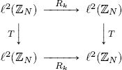
These considerations justify Definition 2.15.
DEFINITION 2.15.– An operator T : ℓ2(ℤN) → ℓ2(ℤN) is said to be stationary (or shift invariant) if:
that is, T is stationary if it commutes with all shift operators Rk:
In section 2.8.5, we shall show that a linear operator T ∈ End ℓ2 ℤN is stationary if and only if ![]() .
.
The DFT provides an extremely important example of a non-stationary operator over ℓ2(ℤN). To prove that the DFT is not a stationary operator, we simply recall the way in which it interacts with shift operators Rk: using formulas [2.30] and [2.33] we obtain, respectively,
which shows that the DFT does not commute with the shift operators.
2.8.1. The DFT and the diagonalization of stationary operators
The most important properties of the DFT with regard to stationary operators can be summarized in a single theorem, but we prefer to highlight the fact that the Fourier transform diagonalizes stationary operators through a separate theorem.
THEOREM 2.8.– Let T ∈ End(ℓ2(ℤN)) be a stationary operator. Then, T is diagonalizable, and each element of the orthogonal Fourier basis Fm of ℓ2(ℤN) is an Eigenvector of T.
PROOF.– For every fixed m ∈ {0, . . . , N − 1}, let us consider the element m of the orthogonal Fourier basis: ![]() .
.
As T is an endomorphism, TFm ∈ ℓ2(ℤN), and thus TFm can be decomposed over the basis (F0, . . . , FN−1) itself :
Now, consider the action of the shift operator R1 on Fm:
Applying T to R1Fm, we obtain:
Now, we switch the order of composition of R1 and T :

Since T is stationary, TR1Fm = R1TFm, that is:
and due to the uniqueness of decomposition over a basis:
Let us analyze this equality. If k = m, then equation [2.42] is simply an identity and requires no further discussion. In the case where k ≠ m, we begin by recalling that m, k ∈ {0, . . . , N − 1}, so the cosine and sine of the complex exponentials have their values in only one period, as the next period begins when m, k = N. Then:
and equation [2.42] can be verified if and only if ak = 0 ∀k ≠ m.
Equation [2.41] thus becomes:
that is, Fm is an eigenvector of T with an eigenvalue am given by the m-th coefficient of the decomposition of TFm on the orthogonal Fourier basis. Evidently, the coefficient am is dependent on T.
Given that we fixed an arbitrary index m, every element of the orthogonal Fourier basis is an eigenvector of T, and consequently ℓ2(ℤN) has a basis of eigenvectors of T. By definition, T is therefore diagonalizable. □
Theorem 2.9 shows how the eigenvalues am can be made explicit using the DFT.
The theorem shown above can be interpreted using matrices. We know that the action of the DFT is represented by the Sylvester matrix WN defined in equation [2.23] and that WN is the matrix used to pass from the canonical basis B of ℓ2(ℤN) to the Fourier basis F of ℓ2(ℤN); the inverse is ![]() , representing the matrix used to pass from basis F to basis B.
, representing the matrix used to pass from basis F to basis B.
If A is the matrix associated with T with respect to the canonical basis of ℓ2(ℤN) and D is the diagonal matrix of the eigenvalues of A, then:
If [w]F represents any vector w ∈ ℓ2(ℤN) with respect to the Fourier basis F , then:
so WNA = DWN, if and only if ![]() .
.
2.8.2. Circulant matrices
Thanks to the introduction of the concept of circulant matrix, we will be able to prove the fundamental theorem concerning the link between the Fourier transform and stationary operators.
First, let us generalize the periodicity of sequences ℓ2(ℤN) to matrices: given a matrix ![]() , we say that A is an N-periodic matrix if:
, we say that A is an N-periodic matrix if:
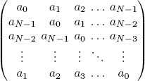
DEFINITION 2.16.– Let ![]() be an N × N periodic matrix. A is said to be circulant if:
be an N × N periodic matrix. A is said to be circulant if:
Repeating the translation k times, the definition is rewritten as:
We see that, since k ∈ ℤ, a circulant periodic matrix can also be defined with the property am−k,n−k = am,n, k ∈ ℤ.
This definition is interpreted as follows. Line (column) m + 1 (n + 1) is obtained from line (column) m (n) by shifting one position to the right (at the bottom), as follows:
2.8.3. Exhaustive characterization of stationary operators
Theorem 2.9 is the most important result of this chapter. It is used to produce the eigenvalues of a stationary operator T in a very simple manner; it can also be used to characterize T as a convolution operator, in the original representation of z, and as a multiplier, in the frequency representation.
THEOREM 2.9.– Let T : ℓ2(ℤN) → ℓ2(ℤN) be an endomorphism. The following properties are equivalent.
- 1) T is stationary.
- 2) The matrix A, which represents T in the canonical basis of ℓ2(ℤN), is circulant.
- 3) T is a convolution operator.
- 4) T is a Fourier multiplier.
- 5) The matrix D, which represents T in the orthogonal Fourier basis F, is diagonal.
Note that implication 1) ![]() 5) has already been proved. The theorem will be proved using the following strategy:
5) has already been proved. The theorem will be proved using the following strategy:
The proof of this theorem is crucial, as it provides an explicit technique for finding the Eigenvalues of T and for constructing the convolution operator and Fourier multiplier which represent T.
PROOF.– ![]() : let A be the associated matrix of T with respect to the canonical basis8
: let A be the associated matrix of T with respect to the canonical basis8 ![]() :
:

From the definition of the associated matrix, we have am,n = (Ten)(m), that is, the n-th column of A is the vector Ten.
Using the fact that T is stationary, we wish to show that:
We see that:

thus en+1 = R1en and, consequently:

Since am+1,n+1 = am,n ∀m, n ∈ ℤN, then A is circulant and the implication ![]() is proved.
is proved.
![]() : let A be a periodic circulant matrix, that is, am,n = am−k,n−k ∀n, m, k ∈ ℤ. We wish to prove the existence of h ∈ ℓ2(ℤN) such that Az = z * h = Th(z) ∀z ∈ ℓ2(ℤN).
: let A be a periodic circulant matrix, that is, am,n = am−k,n−k ∀n, m, k ∈ ℤ. We wish to prove the existence of h ∈ ℓ2(ℤN) such that Az = z * h = Th(z) ∀z ∈ ℓ2(ℤN).
We shall prove that the sequence h which we are looking for is the first column in A, that is:
We see that ![]() and thus, from the definition of the matrix-vector product, we have:
and thus, from the definition of the matrix-vector product, we have:
and implication ![]() is proved.
is proved.
![]() : we must prove that a convolution operator Tw is stationary, that is: (Tw ∘ Rk)(z) = (Rk ∘ Tw)(z), ∀z ∈ ℓ2(ℤn), ∀k ∈ ℤ
: we must prove that a convolution operator Tw is stationary, that is: (Tw ∘ Rk)(z) = (Rk ∘ Tw)(z), ∀z ∈ ℓ2(ℤn), ∀k ∈ ℤ
We begin by calculating the left side of the equation:
Making the index substitution ℓ = n − k ⇔ n = k + ℓ , the variability of ℓ is:

then:
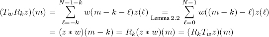
and this proves the implication ![]() .
.
![]() : we must prove that a linear operator T : ℓ2(ℤN) → ℓ2(ℤN) is a convolution operator if and only if T is a Fourier multiplier.
: we must prove that a linear operator T : ℓ2(ℤN) → ℓ2(ℤN) is a convolution operator if and only if T is a Fourier multiplier.
Taking an arbitrary fixed element w ∈ ℓ2(ℤN), we have:

where Mŵ is the multiplication operator by the sequence ŵ. Inversely:

This shows us that the convolution operator with w can be interpreted as the Fourier multiplier by ŵ and vice versa, and that the Fourier multiplier by w can be interpreted as the convolution operator with w̌:
The double implication ![]() is thus proved.
is thus proved.
Before continuing on to the final stage in our proof, let us summarize our findings. A stationary operator T : ℓ2(ℤN) → ℓ2(ℤN) is represented by a circulant matrix A with respect to the canonical basis (e0, . . . , eN−1) of ℓ2(ℤN).
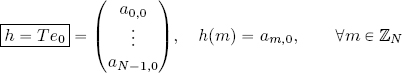
This matrix A can be represented by the convolution operator Th with h = Te0, the first column of A or, as we have just seen, by the Fourier multiplier T(ĥ), where ĥ is the sequence of Fourier coefficients of h.
![]() : we must prove that T is a Fourier multiplier T(w) if and only if the associated matrix of T with respect to the orthogonal Fourier basis F is diagonal.
: we must prove that T is a Fourier multiplier T(w) if and only if the associated matrix of T with respect to the orthogonal Fourier basis F is diagonal.
The direct implication has already been proved in formula [2.27], so we simply need to prove the implication 5) ![]() 4). Stating that D = diag(dn,n), n = 0, . . . , N − 1 is the diagonal matrix which represents an operator T in the Fourier basis F means that:
4). Stating that D = diag(dn,n), n = 0, . . . , N − 1 is the diagonal matrix which represents an operator T in the Fourier basis F means that:
with Mw the multiplication operator by the sequence w(n) = dn,n, n = 0, . . . , N −1. Applying the IDFT to both sides:
hence T = T(w) proving the implication 5) ![]() 4).
4).
The proof of the theorem is now complete. □
The theorem demonstrated above provides a standard technique for studying stationary operators T over ℓ2(ℤN). We recall that the sequence:
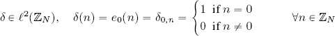
is the unit pulse; thus, operator T is completely determined by its action on δ, h = T δ, which is referred to as the unit pulse response. ĥ, the DFT of the unit pulse response, is called the transfer function.
The properties demonstrated in theorems 2.8 and 2.9 can be used to summarize the analysis of stationary operators, as shown in Box 2.2.
Box 2.2. Analysis of stationary operators over ℓ2(ℤN)
2.8.4. High-pass, low-pass and band-pass filters
The synthesis formula for any given signal z ∈ ℓ2(ℤN) transformed) via the action of a stationary operator T ∈ End(ℓ2(ℤN)) is:
where Fm is the vector with index m of the orthogonal Fourier basis of ℓ2(ℤN). Thus, ![]() represents the importance of the harmonic of frequency m in the reconstruction of Tz, and
represents the importance of the harmonic of frequency m in the reconstruction of Tz, and ![]() represents the spectrum of the transformed signal Tz.
represents the spectrum of the transformed signal Tz.
To understand how the spectrum of Tz is linked to that of the original signal z, let us apply the DFT to both sides of the formula Tz = T(ĥ) z = IDFT (ĥ · ẑ), where h = T δ0:
that is:
so the Fourier coefficients of Tz, the sequence transformed by the operator T, are given by the product of the Fourier coefficients of the original sequence z and the Fourier coefficients of the unit pulse response h.
Consequently, the spectrum of the transformed sequence Tz is:
This allows us to understand the action of stationary filters T on the frequency content of a signal z:
– if ĥ(0) = 0, the average of Tz is zero, since ![]() and we know that
and we know that ![]() is proportional to the average of Tz;
is proportional to the average of Tz;
– if |ĥ(0)| = 1, then T preserves the average of z, that is 〈Tz〉 = 〈z〉 ;
– if |ĥ(m)| > 1 for m ≃ 0 and m ≃ N −1, and |ĥ(m)| ∈ [0, 1[ for m ≃ N/2, then T increases the low frequencies and reduces the high frequencies (low-pass filter);
– if |ĥ(m)| > 1 for m ≃ N/2 and |ĥ(m)| ∈ [0, 1[ for m ≃ 0 and m ≃ N −1, then T increases the high frequencies and reduces the low frequencies (high-pass filter);
– if |ĥ(m)| > 1 for intermediate values of m, then T increases the mid-range frequencies (band-pass filter).
2.8.5. Characterizing stationary operators using shift operators
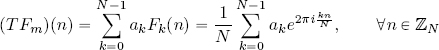
We now have all of the results we need to demonstrate the characterization of a stationary operator as a linear combination of shift operators, or, in an equivalent manner, as a polynomial of the shift operator R1, since Rk = R1 ∘ · · · ∘ R1 k times, that is, ![]() .
.
THEOREM 2.10.– T ∈ End(ℓ2(ℤN)) is stationary if and only if the expression of T is:
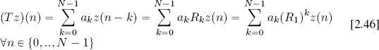
where ak ∈ ![]() .
.
PROOF.–
![]() : let T be stationary. We know that T = Th, where Th is the convolution operator with regard to the unit pulse response h = T δ, that is:
: let T be stationary. We know that T = Th, where Th is the convolution operator with regard to the unit pulse response h = T δ, that is:
We must therefore simply identify the coefficients ak of the formula ![]() with h(k) to obtain our thesis.
with h(k) to obtain our thesis.
![]() : we can verify that T, written in the form used in formula [2.46], is stationary due to the linearity of T and Rk. We know that ∀n ∈ {0, . . . , N − 1}:
: we can verify that T, written in the form used in formula [2.46], is stationary due to the linearity of T and Rk. We know that ∀n ∈ {0, . . . , N − 1}:
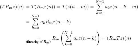
hence: T ∘ Rm = Rm ∘ T ∀m ∈ ℤ.
Since h(k) = T δ(k), the proof of the theorem above also proves the validity of the formula:

2.8.6. Frequency analysis of first and second derivation operators (discrete case)
In this section, we shall analyze two stationary operators which represent the discrete version of the first and second derivatives. By comparing their eigenvalues, we see that the second derivation operator is more efficient for amplifying high frequencies in digital signals.
DEFINITION 2.17.– Given a sequence z ∈ ℓ2(ℤN), we define:
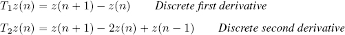
The discrete first derivative is simply the forward difference of z, divided by the difference of the values of n, but since (n + 1) − n = 1 there is no need to write the denominator.
The discrete second derivative is the backward difference of the discrete first derivative of z, divided by the difference of the values of n, which – once again – is 1, so does not need to be written: T2z(n) = T1z(n) − T1z(n − 1) = z(n + 1) − z(n) − [z(n) − z(n − 1)] = z(n + 1) − 2z(n) + z(n − 1).
Let us begin by analyzing T1. To calculate the pulse response, T1 is applied to the unit pulse δ = e0:

using the fact that e0(0) = e0(N) = 1. The matrix which represents T1 in the canonical basis of ℓ2(ℤN) is:

Now, let us calculate the DFT of h. For all m ∈ ℤN, this is:
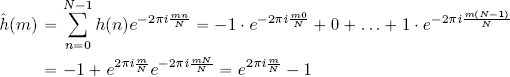
so the eigenvectors of T1 are ![]() and its diagonal representation is:
and its diagonal representation is:
The action of T1 in terms of frequency can now be interpreted using formula [2.45]. We wish to calculate the magnitudes of the Eigenvalues (ĥ(m))m∈ZN . We see that:
Thus, ![]() , while
, while ![]() , so the sinus is always non-negative and the absolute value can be eliminated. To summarize:
, so the sinus is always non-negative and the absolute value can be eliminated. To summarize:
Specifically:
– |ĥ(0)| = 0: hence, the filtered signal T1z averages to zero;
– ![]() ;
;
– ![]() ;
;
– |ĥ(m)| → 0 if m → 0 or m → N − 1;
– the action of the operator is symmetrical with regard to ![]() .
.
Since m = N/2 represents the highest frequency of the signal and m = 0 and m = N − 1 represent the lowest frequencies, we can deduce that T1 reduces the low frequencies of z and increases the high frequencies by up to two times. Thus, the discrete first derivative operator is a high-pass filter.
Now, let us analyze T2. Its pulse response is given by the vector:

The matrix associated with T2 in the canonical basis of ℓ2(ℤN) is:

Next, we calculate the DFT of h :
These values of ĥ(m) must now be compared with those of the first derivative operator. We do this by rewriting ![]() and using the trigonometric identity
and using the trigonometric identity ![]() with
with ![]() to obtain
to obtain ![]() . The eigenvalues of T2 are thus
. The eigenvalues of T2 are thus ![]() , m = 0, 1, ..., N − 1, and its diagonal representation is:
, m = 0, 1, ..., N − 1, and its diagonal representation is:
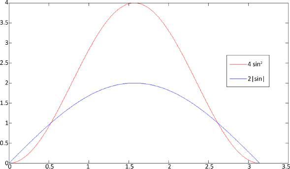
Figure 2.4. Difference between the sine functions representing the spectrum values of the first and second derivative operators between 0 and π. For a color version of this figure, see www.iste.co.uk/provenzi/spaces.zip
The effect of T2 on the frequency is defined by the magnitudes of its Eigenvalues:
We see that the magnitudes of the Eigenvalues of the second derivative operator are the squares of those of the first derivative operator. Hence:
– |ĥ(0)| = 0: thus, as in the case of the first derivative, the filtered signal T2z averages to zero;
– ![]() ;
;
– ![]() ;
;
– |ĥ(m)| → 0 if m → 0 or m → N − 1 and the convergence to zero is faster than for the first derivative operator, as in this case, the sine is squared, as illustrated in Figure 2.4;
– The action of the operator is symmetrical about ![]() .
.
Thus, the discrete second derivative operator is also a high-pass filter, amplifying high frequencies and reducing low frequencies in a way which is the square of the action of the discrete first derivative operator.
2.9. The two-dimensional discrete Fourier transform (2D DFT)
The Fourier transform considered up to now applies to signals z(n) which depend on only one parameter n.
In practical contexts, signals are often very large and depend on multiple parameters. One classic example is that of digital images, which include two parameters: the two spatial coordinates of a pixel, as shown in Figure 2.5.
DFT theory can be generalized for signals which depend on any (finite) number of parameters. For simplicity’s sake, we shall focus on the two-dimensional (2D) case, with parameters n1, n2.
The first step is to introduce the domain vector space: if N1, N2 ∈ ℕ, we define:
z ∈ ℓ2(ℤN1 × ℤN2) is a complex sequence which depends on two parameters:
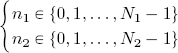

Figure 2.5. The two coordinates of a pixel, n1, n2, in a digital image (image source: author). For a color version of this figure, see www.iste.co.uk/provenzi/spaces.zip
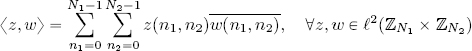
ℓ2(ℤN1 × ℤN2) is a vector space of dimension N1 · N2. The definitions used for summation and multiplication by a complex scalar are the same as those used for the 1D case and for inner products:
To extend DFT theory from one to two dimensions, we use the procedure for generating bases in ℓ2(ℤN1 × ℤN2) from bases in ℓ2(ℤN1) and ℓ2(ℤN2).
THEOREM 2.11.– Let {B0, B1, . . . , BN1−1}, {C0, C1, . . . , CN2−1} be orthonormal bases in ℓ2(ℤN1) and ℓ2(ℤN2), respectively.
For all m1 ∈ {0, . . . , N1 − 1} and m2 ∈ {0, . . . , N2 − 1}, consider the sequences in ℓ2(ℤN1 × ℤN2) given by:
Then, Dm1,m2 is an orthonormal basis of ℓ2(ℤN1 × ℤN2), known as the tensor product basis of the two original bases.
PROOF.– The sequences Dm1,m2, m1 ∈ {0, . . . , N1 − 1} and m2 ∈ {0, . . . , N2 − 1} are N1 · N2 elements of ℓ2(ℤN1 × ℤN2), which is of dimension N1 · N2. Proof that these constitute an orthonormal basis can be obtained by showing that:

For m1 ∈ {0, 1, . . . , N1 − 1} and m2 ∈ {0, 1, . . . , N2 − 1}, this theorem has the following corollaries:
– the canonical orthonormal basis of ℓ2(ℤN1 × ℤN2) is:

– the orthogonal Fourier basis of ℓ2(ℤN1 × ℤN2) is:

– the orthonormal Fourier basis of ℓ2(ℤN1 × ℤN2) is:
– the orthogonal basis of the complex exponentials in ℓ2(ℤN1 × ℤN2) is:
Using the theory of complex inner product spaces, the definition of Fourier coefficients, the DFT and the IDFT can be generalized to ℓ2(ℤN1 × ℤN2). Taking z ∈ ℓ2(ℤN1 × ℤN2), we have:
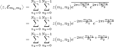
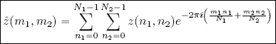
thus the Fourier coefficients of z ∈ ℓ2(ℤN1 × ℤN2) are defined as follows:
As in the 1D case:
where 〈z〉 is the average of z. Note that the quantity N1N2 may be extremely large.
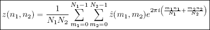
The synthesis formula can also be generalized to the 2D case, as follows:
The 2D DFT and 2D IDFT operators can therefore be written using the following formulas:

and:

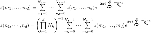
Clearly, if the dimension is increased from 2 to 2 < d < +∞, these formulas can be generalized in the following manner:
2.9.1. Matrix representation of the 2D DFT: Kronecker product versus iteration of two 1D DFTs
The matrix representation of the 2D DFT in the canonical basis of ℓ2(ℤN1 × ℤN2) can be constructed using the Sylvester matrices WN1 and WN2 associated with the 1D DFT for ℓ2(ℤN1) and for ℓ2(ℤN2), respectively.
The operation used to obtain a matrix representation of the 2D DFT is the Kronecker product, which is defined below.
DEFINITION 2.18.– Given two matrices, A of dimension m × n and B of dimension p × q:
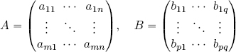
the Kronecker product matrix A ⊗ B is the matrix of dimension mp × nq defined by:
The matrix associated with the 2D DFT in the canonical basis of ℓ2(ℤN1 × ℤN2) can be shown, by direct calculation, to be the matrix of dimension N1N2 × N1N2 given by:
Unfortunately, the calculation needed to obtain the Kronecker product matrix becomes unfeasibly large for high values of N1 and N2. In practice, the 2D DFT is generally written as the iteration of two 1D DFTs.
To understand this approach, z ∈ ℓ2(ℤN1 × ℤN2) must be interpreted as a matrix made up of N2 column vectors with N1 elements:

N1 elements for each column vector
From the definition of the 2D DFT, we can write:

In this formula, the sum with regard to index n2 is the furthest out, so n2 is fixed each time. Taking a fixed value for n2, z(n1, n2) is a column vector, so the highlighted parenthesis represents the 1D DFT of the column vector, which can be obtained by applying matrix WN1 to z(n1, n2), with a fixed value of n2, as before.
The next problem is that n1 is fixed, and the changing index is n2, meaning that WN1 z(n1, n2) is a row vector. For this reason, the DFT cannot be obtained by applying WN2: as we saw in section 2.5, the 1D DFT is obtained from the product of the matrix WN and a sequence represented using a column vector.
The solution to this problem consists of transposing the two sides of equation [2.47], transforming the row vector ẑ(m1, n2) into a column vector:

Now, (WN1z(n1, n2))t is a column vector, so the DFT can be calculated by applying WN2 :

since ![]() (note that n1 and n2 have swapped places). Thus, ẑ(m1, m2)t = WN2 z(n2, n1) WN1, so to find ẑ(m1, m2), we must simply transpose both sides again:
(note that n1 and n2 have swapped places). Thus, ẑ(m1, m2)t = WN2 z(n2, n1) WN1, so to find ẑ(m1, m2), we must simply transpose both sides again:
The formula used to calculate the 2D DFT of a sequence z ∈ ℓ2(ℤN1 × ℤN2) is thus:
It is important to note that equation [2.48] is only meaningful if ẑ(m1, m2) and z(n1, n2) are interpreted as N1 × N2 matrices in their entirety.
Formula [2.48] is not the same as WN1WN2z(n1, n2) or WN2WN1z(n1, n2), i.e. the formulas that one could have naively thought to use to implement 1D DFT over the columns and rows of z. The reason for this difference, as we have seen, is that the 1D matrix DFT requires the presence of a column vector, hence the transposition which results in formula [2.48].
2.9.2. Properties of the 2D DFT
The generalization of the properties of the 1D DFT, presented in section 2.7, to the 2D DFT is trivial.
The demonstrations of these properties in 1D and 2D are practically identical, notwithstanding certain differences in notation. For this reason, we shall not provide proofs for the 2D extensions presented below.
As in the 1D case, in order to examine the properties of the 2D DFT, we must first extend the definition of a sequence z ∈ ℓ2(ℤN1 ×ℤN2) by periodicity to any interval of length N1 with regard to the variable n1 and of length N2 with regard to the variable n2.
This extension is possible if z is defined outside of ℤN1 × ℤN2 in the following manner:
The shift operator is also helpful in 2D cases.
DEFINITION 2.19.– Take z ∈ ℓ2(ℤN1 × ℤN2), extended by periodicity as in formula [2.49], and k1, k2 ∈ ℤ. The shift operator over ℓ2(ℤN1 × ℤN2) is defined by:

Box 2.3. Properties of 2D DFT
2.9.3. 2D DFT and stationary operators
The properties of 2D and 1D DFT with regard to stationary operators are the same.
Strictly speaking, an operator T : ℓ2(ℤN1 × ℤN2) → ℓ2(ℤN1 × ℤN2) is stationary if:
In practice, if z is a digital image, a stationary operator is a transformation whose action is independent of the position of a pixel in the spatial context of the image.
As in the 1D case, stationary operators over ℓ2(ℤN1 × ℤN2) may be characterized as convolution operators or as Fourier multiplier operators.
The theorem formalizing this relation relies on definitions of the Fourier multiplier, the unit pulse and the pulse response in the 2D case.
DEFINITION 2.20.– Taking a fixed w ∈ ℓ2(ℤN1 × ℤN2), the Fourier multiplier associated with w is defined as:
DEFINITION 2.21.– The unit pulse δ in ℓ2(ℤN1 × ℤN2) is the first vector in the canonical basis: δ = e0,0.
Given a linear operator T over ℓ2(ℤN1 × ℤN2), the pulse response is defined as the sequence h = T δ ∈ ℓ2(ℤN1 × ℤN2).
THEOREM 2.12.– Let T : ℓ2(ℤN1 × ℤN2) → ℓ2(ℤN1 × ℤN2) be a linear operator. The following conditions are equivalent:
1) T is stationary;
2) T is the convolution operator with the pulse response h = T δ:
3) T is the Fourier multiplier associated with ĥ :
4) T is diagonalizable, its eigenvectors are the orthogonal Fourier basis Fm1,m2 of ℓ2(ℤN1 × ℤN2), and its eigenvalues are the components of ĥ.
OBSERVATIONS.– This result can be extended to circulant matrices, but their definition in the 2D case is more complex.
2.9.4. Gradient and Laplace operators and their action on digital images
Repeating the analysis of discrete derivative operators from section 2.8.6 for 2D cases, the first derivative gives us the gradient, that is ![]() , and the second derivative gives us the Laplacian, that is
, and the second derivative gives us the Laplacian, that is ![]() .
.
The gradient is used to detect the edges of an image in a particular direction. For isotropic edge detection – that is detection which is uniform with regard to direction – the Laplacian is used; this approach is more efficient than using a gradient for intensifying fine details, as we saw in the 1D case.
Even in 2D cases, the differential operators above cancel out the average of an image, which is why the output is entirely black, except near the edges, as we see from Figure 2.6.
2.9.5. Visualization of the amplitude spectrum in 2D
Visualizations of the spectrum of a 2D signal can be produced on the condition that the signal is centered, for the same reasons presented in the 1D case. Centering may be carried out using the 2D equivalent of formula [2.34], considering (−1)n1+n2z (n1, n2) in the place of z(n1, n2), as we saw in section 2.9.2.
Note that the 1D symmetry of the 1D DFT with regard to frequencies m ∈ {0, 1, . . . , N/2} and m ∈ {N/2 + 1, N/2 + 2, . . . , N − 1} is replaced by 2D mirror symmetry in the case of the 2D DFT.
Figure 2.7 shows three grayscale digital images with their amplitude spectrums. The brightest points correspond to high magnitude values of the Fourier coefficients, while the darkest points correspond to low values.
There are several notable characteristics here:
– the symmetry of the spectrum: frequency content is repeated in each quadrant by mirror symmetry;
– the brightest points are located toward the center of the spectrum: this is due to the fact that these spectrums are centered, so the coordinates of the central frequency are (m1, m2) = (0, 0) and |ẑ(0, 0)| = N1N2〈z〉, that is, N1N2 times the average value of the image. This is why a compressive function, such as a logarithm, must be used to visualize a spectrum: the values of |ẑ(0, 0)| are so much higher than the others that the variability range needs to be compressed;

Figure 2.6. a) Original image of Panko; b) image after Laplacian filter; c) image filtered using a gradient in the vertical direction; d) image filtered using a gradient in the horizontal direction (image source: author). For a color version of this figure, see www.iste.co.uk/provenzi/spaces.zip
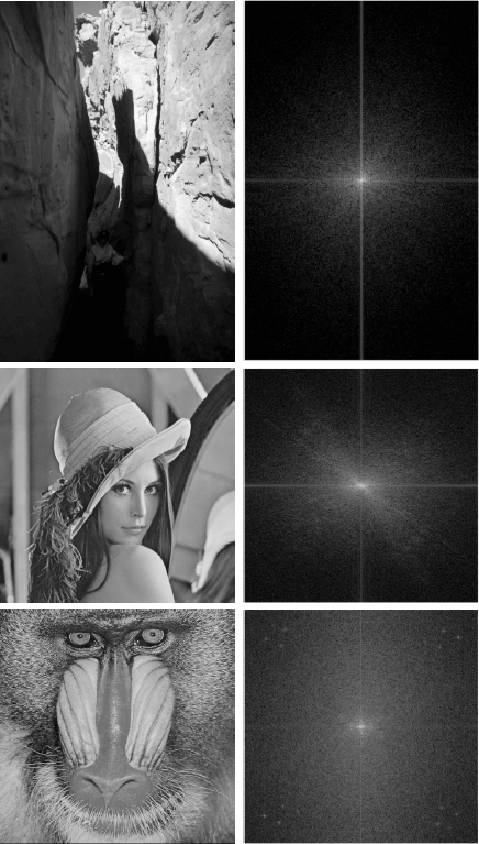
Figure 2.7. Left column: original images. Right column: centered amplitude spectrums of the images in the left column, visualized using a logarithmic scale
– moving out from the center, the spectrum shows the amplitude of the coefficients corresponding to the highest frequencies, up to the maximum frequencies (N1/2, N2/2), if N1, N2 are even, or their integer parts ([N1/2] , [N2/2]) if N1, N2 are odd. The image with the highest frequency content is that of the mandrill: its spectrum is the widest of the three shown here. Note the particularly intense values near the edges, representing very high frequencies: these correspond to the fine details of the hairs near the animal’s eyes;
– as m1 and m2 represent vertical and horizontal frequencies, the vertical and horizontal edges of the images produce Fourier coefficients which are localized on the corresponding axes. This is why the spectrum of the first image, which features strong vertical intensity gradients between the rocks and the sea, is heavily dominated by intense Fourier coefficients on the vertical axis. The second image (“Lena”, a classic image used in image processing) features fine details in the hat area, at 45° and −45°. This results in evident diagonal structures in the spectrum;
– from this spectrum analysis, we see that the Fourier spectrum reveals the presence of geometric structures within an image, but does not tell us where in the image these structures are located.
2.9.6. Filtering: an example of digital image filtering in a Fourier space
Theorem 2.12 states that all stationary operators T acting on images (interpreted as finite 2D sequences) are “hidden” convolutions between the image and the pulse response h = T δ.
Furthermore, these convolutions can be represented as Fourier multipliers (multiplication of ĥ and the 2D DFT of the image within the Fourier space).
Different results will be obtained depending on the sequence h with which convolution is carried out. The effect of a convolution is often easier to interpret by examining the associated Fourier multiplier.
Let us consider the notion of convolution with a discrete Gaussian, noted h(n1, n2).
As we shall see in Chapter 6, the Fourier transform of a Gaussian with a standard deviation σ is itself a Gaussian, but the standard deviation of the latter is inversely proportional to σ. Thus, we can further our understanding of the meaning of convoluting an image z(n1, n2) with a Gaussian h(n1, n2) by analyzing the multiplication ẑ(m1, m2) · ĥ(m1, m2) in the Fourier space.
Figure 2.8 features three images corresponding to 512 × 512 2D Gaussians. The intensity of the pixel in position (n1, n2) is ![]() and the standard deviation is σ =1, 5 and 10, respectively.
and the standard deviation is σ =1, 5 and 10, respectively.
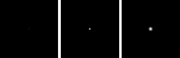
Figure 2.8. Two-dimensional Gaussian images with a standard deviation of (left - right) 1, 5 and 10
As we stated above, the 2D DFTs of h are still Gaussians, but their standard deviations are proportional to 1, ![]() , and
, and ![]() . Evidently, h(0, 0) = 1 and the values of ĥ(m1, m2) decrease as we move away from the center; thus, multiplication in the Fourier space ẑ(m1, m2) · ĥ(m1, m2) decreases the importance of the harmonics with (m1, m2) ≠ (0, 0), which are associated with the finer details in the image. Applying the 2D IDFT to ẑ(m1, m2) · ĥ(m1, m2), we can reconstruct an image which is blurrier than the original.
. Evidently, h(0, 0) = 1 and the values of ĥ(m1, m2) decrease as we move away from the center; thus, multiplication in the Fourier space ẑ(m1, m2) · ĥ(m1, m2) decreases the importance of the harmonics with (m1, m2) ≠ (0, 0), which are associated with the finer details in the image. Applying the 2D IDFT to ẑ(m1, m2) · ĥ(m1, m2), we can reconstruct an image which is blurrier than the original.
In image processing, convolution with a Gaussian corresponds to a blurring operation, as we see in Figure 2.9.

Figure 2.9. Blurred image of Lena obtained by multiplying DFTs and Gaussians with standard deviations of (left - right) 1, 5 and 10
COMMENT CONCERNING FIGURE 2.9.– Note that as the standard deviation of the DFT of a Gaussian is inversely proportional to the original standard deviation, the DFT of the Gaussian with a standard deviation of 10 has a small standard deviation in the latter case, and thus tends rapidly toward 0. So, when the DFT of the Gaussian with an SD of 10 is multiplied with the DFT of the image, much of the detail in the image is lost.
Blurring has a number of uses; for example, in cases where the original image is noisy, blurring can make this noise less evident (although it also reduces edge sharpness).
Figure 2.10 shows a continuous version of the blurring frequency filter.
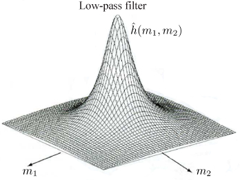
Figure 2.10. Blurring filter/low-pass filter in the frequency domain
NOTE.– Although convolution with a Gaussian results in a blurring effect, it would be wrong to assume that convolution is always associated with a blurring action. As we saw earlier, convolution, alongside the Fourier multiplier, constitutes a prototype for all stationary operators, which may blur a signal or enhance its contrast.
2.10. Summary
In this chapter, we considered the space ℓ2(ℤN) composed of ℕ-periodic sequences with complex values, isomorphic to ![]() N.
N.
We introduced a special basis in this space, made up of the complex exponentials generated by the consecutive powers of the N-th complex roots of the unit. This basis is used to construct the Fourier basis of ℓ2(ℤN). We interpreted the elements of this basis as harmonic waves, oscillating at frequencies which are multiples of a fundamental one.
The Fourier coefficients of an element in ℓ2(ℤN) are its components with regard to the Fourier basis. As these coefficients are complex, their magnitude must be used to determine the importance of a harmonic in relation to a certain frequency when reconstructing (or synthesizing) the element itself. The set of magnitudes of the Fourier coefficients is known as the spectrum of an element in ℓ2(ℤN).
The DFT is the endomorphism of ℓ2(ℤN) which associates an element of ℓ2(ℤN) with the sequence of its Fourier coefficients. The DFT is actually an isomorphism, and its inverse is known as the IDFT.
The DFT may be associated with a matrix, known as a Sylvester matrix; this matrix is a Vandermonde matrix, that is, all of the lines and columns in the matrix can be obtained through geometric progressions.
We presented an interpretation of these concepts in the context of signal theory, notably highlighting the fact that the highest harmonic oscillation frequency in a discrete signal obtained from N samples is N/2 (or half of its integer part if N is odd); this is the Nyquist frequency.
The DFT transforms the shift operation into a multiplication by a phase factor, that is, a complex exponential with unit magnitude; this implies that the signal spectrum is shift-invariant.
Convolution is transformed by the DFT into a pointwise product, allowing the convolution operator to be expressed diagonally in the Fourier space.
Finally, we saw that the DFT can be used to diagonalize stationary operators, that is, operators which commutate with shift operators. theorem 2.9 can be used to fully characterize a stationary operator as a convolution or as a Fourier multiplier and to determine the eigenvalues of this operator.
- 1 James Joseph Sylvester (1814, London-1897, London).
- 2 A geometric progression of reason r is the sequence of powers 1 = r0, r = r 1, r 2, r 3, . . . , r n.
- 3 Alexandre-Théophile Vandermonde (1735, Paris-1796, Paris).
- 4 This is the real Euclidean product of the m-th line of WN, i.e. ( wm0 wm1, . . . , wm(N − 1)) times the components (z (0), z (1), . . . , z(n)) of z.
- 5 It is important to specify that these harmonics are discrete; continuous harmonics are obtained using functions t ↦ e2πimvt = eimwt, where ν is the frequency and w = 2πν the pulse.
- 6 The magnitude must be used here due to the fact that complex numbers are not ordered.
- 7 For the Swedish engineer Harry Nyquist (1889–1976).
- 8 We recall that en(m) = δn,m, ∀n, m ∈ ℤN.