3
Lebesgue’s Measure and Integration Theory
In this chapter, we shall present the most essential elements of measure theory and integration. Our aim here is simply to establish clear and unambiguous notation and a common vocabulary.
What follows is a deliberately brief summary. Readers who have not yet studied this important branch of mathematics may wish to look elsewhere for a more detailed introduction to measure theory and integration.
Two excellent reference works in this domain are Briane and Pagès (1998) and Bartle (1966).
3.1. Riemann versus Lebesgue
The main difference between the Riemann and Lebesgue approaches is shown in Figure 3.1.
The key to Riemann integration lies in approximating the area of the surface between the x axis and the curve of a function f using small rectangles [ai−1, ai] × [0, Φi] with their base on the x axis, of a height Φi close to the average height of function f over [ai−1, ai].
Lebesgue’s integration theory differs in that the first stage involves breaking down the y axis into small intervals [bj−1, bj]; the surface below the curve f is then approximated using:
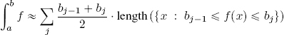

Figure 3.1. Riemann and Lebesgue integration. For a color version of this figure, see www.iste.co.uk/provenzi/spaces.zip
The main difficulty lies in the fact that the sets:
shown in red in Figure 3.1(b), are generally not intervals, and it can be complicated, if not (as in certain cases) impossible, to associate them with a length or measure.
The development of measure theory was motivated by the need to create a theory of integration using the strategy described above. This approach is far longer and more complicated than Riemann integration; however, Lebesgue integration presents a significant advantage in terms of generality, and the properties that can be proved are far more powerful.
3.2. σ-algebra, measurable space, measures and measured spaces
In order to define a Lebesgue integral, we must first define the sets and functions which can be measured. The definitions and results below, based on work carried out in the early 20th century, make up the necessary formalization.
Let X be a set. A σ-algebra on X is a collection ![]() of subsets of X, that is
of subsets of X, that is ![]() ⊆
⊆ ![]() (X), which verifies the following properties:
(X), which verifies the following properties:
– ∅, X ∈ ![]() ;
;
– ![]() is closed under complementation: E ∈
is closed under complementation: E ∈ ![]()
![]() Ec ∈
Ec ∈ ![]() ;
;
– ![]() is closed under countable unions:
is closed under countable unions: ![]() .
.
This definition implies that ![]() is closed under countable intersection.
is closed under countable intersection.
Mathematicians working on measure theory have proved that the defining properties of a σ-algebra are necessary and sufficient to “measure” the sets contained in the σ-algebra itself, in a sense which will be defined below. For this reason, the pair (X, ![]() ) is called a measurable space and the elements of
) is called a measurable space and the elements of ![]() are measurable sets.
are measurable sets.
One further concept must be introduced before we can examine a meaningful example of a measurable space: that of the ordering relation between σ-algebras. If every element in a σ-algebra ![]() 1 is contained in the σ-algebra
1 is contained in the σ-algebra ![]() 2, then
2, then ![]() 1 is said to be smaller than
1 is said to be smaller than ![]() 2 and we write
2 and we write ![]() 1 ⊂
1 ⊂ ![]() 2. This concept is used to define the smallest σ-algebra generated by a collection of power sets: taking S ⊂
2. This concept is used to define the smallest σ-algebra generated by a collection of power sets: taking S ⊂ ![]() (X), the intersection of all σ-algebras which contain S is known as the σ-algebra generated by S.
(X), the intersection of all σ-algebras which contain S is known as the σ-algebra generated by S.
The case of a topological set X is particularly interesting, and merits closer attention.
The existence of a topology means that we can define the concept of an open part of X. Taking τ ⊆ ![]() (X) to be the open sets of X, we clearly see that τ is not a σ-algebra, since the complement of an open set is a closed set. However, we can consider the σ-algebra generated by τ , called the Borel σ-algebra1and noted
(X) to be the open sets of X, we clearly see that τ is not a σ-algebra, since the complement of an open set is a closed set. However, we can consider the σ-algebra generated by τ , called the Borel σ-algebra1and noted ![]() (X). Each element in this algebra – which is a subset of X – is called a Borel set.
(X). Each element in this algebra – which is a subset of X – is called a Borel set.
Once we have a measurable space (X, ![]() ), the concept of a positive measure, or simply a measure, μ can be defined as a function μ :
), the concept of a positive measure, or simply a measure, μ can be defined as a function μ : ![]() → [0, +∞] such that:
→ [0, +∞] such that:
– μ(∅) = 0 ;
– μ is σ-additive (or countably additive): if (En)n∈ℕ is a countable family of two-by-two disjoint elements in ![]() , then:
, then:
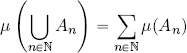
The triple (X, ![]() , μ) is said to be a measure space. When the σ-algebra
, μ) is said to be a measure space. When the σ-algebra ![]() and the measure μ are clearly specified, they are often omitted and one simply writes X.
and the measure μ are clearly specified, they are often omitted and one simply writes X.
One very simple, but meaningful, example of a measure is given by the Dirac measure in the measurable space (ℝ, ![]() (ℝ)), that is, ℝ with the Borel σ-algebra. The Dirac measure centered on x0 ∈ ℝ is defined by: δx0 :
(ℝ)), that is, ℝ with the Borel σ-algebra. The Dirac measure centered on x0 ∈ ℝ is defined by: δx0 : ![]() (τ) → {0, 1}:
(τ) → {0, 1}:

Since ℝ itself is an element in ![]() (ℝ), δx0(ℝ) = 1, and the Dirac measure of ℝ is 1, independently of the starting point. It is therefore an example of a finite measure, that is, the measure of the entire space is finite.
(ℝ), δx0(ℝ) = 1, and the Dirac measure of ℝ is 1, independently of the starting point. It is therefore an example of a finite measure, that is, the measure of the entire space is finite.
Measures are generally σ-finite, rather than simply finite. Given a measure space (X, ![]() , μ), μ is said to be a σ-finite measure if X can be written as the countable union of measurable sets (En)n∈ℕ ⊂ X with a finite measure, that is:
, μ), μ is said to be a σ-finite measure if X can be written as the countable union of measurable sets (En)n∈ℕ ⊂ X with a finite measure, that is:
Several different techniques exist for constructing a measure, but these are not simple and cannot be described in short form. Readers may wish to consult the volume cited in the preface, or any other work on measure theory.
3.3. Measurable functions and almost-everywhere properties (a.e)
The next step is to introduce the morphisms of measurable spaces, that is, applications between measurable spaces which preserve measurability.
Let (X1, ![]() 1), (X2,
1), (X2, ![]() 2) be two measurable spaces and f : X1 → X2 an arbitrary function. f is a measurable function (with respect to the chosen σ-algebras
2) be two measurable spaces and f : X1 → X2 an arbitrary function. f is a measurable function (with respect to the chosen σ-algebras ![]() 1 and
1 and ![]() 2) if the reciprocal image via f of any element of the σ-algebra
2) if the reciprocal image via f of any element of the σ-algebra ![]() 2 is included in
2 is included in ![]() 1, that is2:
1, that is2:
This is equivalent, by definition, to stating that the reciprocal image via f of a measurable set of X2 (with respect to ![]() 2) is a measurable set of X1 (with respect to
2) is a measurable set of X1 (with respect to ![]() 1).
1).
Let us now recall the crucial concept of properties which are defined almost everywhere. A function f defined on a measure space (X, ![]() , μ) has a property which holds almost everywhere (written a.e.) if f possesses this property on XE, where E ∈
, μ) has a property which holds almost everywhere (written a.e.) if f possesses this property on XE, where E ∈ ![]() has a measure of zero: μ(E) = 0.
has a measure of zero: μ(E) = 0.
3.4. Integrable functions and Lebesgue integrals
Given a measure space (X, ![]() , μ), the integral of a measurable function defined by real or complex functions is relatively simple to obtain. We start by considering a special function, the indicator (or characteristic) function of a set E ∈
, μ), the integral of a measurable function defined by real or complex functions is relatively simple to obtain. We start by considering a special function, the indicator (or characteristic) function of a set E ∈ ![]() : χE : X → {0, 1}:
: χE : X → {0, 1}:
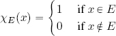
An equivalent notation is ![]() E.
E.
Indicator functions are used to define simple functions or step functions via linear combination. More precisely, taking ![]() to be a finite and disjoint partition of X, that is, Ek ⋂ Ek′ = ∅ ∀k ≠ k′ and
to be a finite and disjoint partition of X, that is, Ek ⋂ Ek′ = ∅ ∀k ≠ k′ and
a simple function s : X → ℝ is defined as:
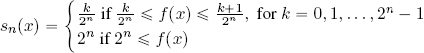
s(x) = ck ∀x ∈ Ek; hence s can only take a finite number of values; if X is a subset of ℝ, then s is a piecewise constant function.
The natural definition of the Lebesgue integral of a simple function is:
Note that, without the definition of the set measure Ek, the integral of s would not be correctly defined.
The importance of simple functions is expressed in Theorem 3.1.
THEOREM 3.1.– Let (X, ![]() , μ) be a measure space and f : X → [0, +∞] a measurable and non-negative function. f can be approximated from below using a series of simple functions, that is, Ǝ (sn)n∈ℕ, with sn a simple function; such that
, μ) be a measure space and f : X → [0, +∞] a measurable and non-negative function. f can be approximated from below using a series of simple functions, that is, Ǝ (sn)n∈ℕ, with sn a simple function; such that ![]() , that is:
, that is:
1) 0 ≼ s0(x) ≼ s1(x) ≼ . . . ≼ sn(x) ≼ . . . ≼ f(x) ∀x ∈ X ;
2) ![]() (pointwise limit). If f is bounded, then the convergence of the sequence (sn)n∈ℕ toward f is uniform.
(pointwise limit). If f is bounded, then the convergence of the sequence (sn)n∈ℕ toward f is uniform.
The proof of this theorem is both elegant and informative, showing that the sequence of simple functions is given by:
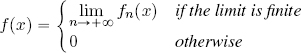
This fundamental theorem makes it possible to define the integral of a measurable non-negative function f : X → [0, +∞] as:
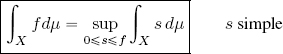
f is said to be (Lebesgue) integrable if ∫X fdμ < +∞.
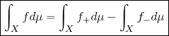
If f : X → ℝ̅ is measurable, then its integral can be defined by considering its positive part:

and its negative part:
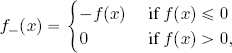
note that both these functions are positive-valued. Since f = f+ − f−, if f+ and f− are integrable, then we can define the integral of a measurable function with extended real values as:
The same strategy is used for measurable functions f : X → ![]() , but using the positive and negative parts of the real part ℜℯ (f) and the imaginary part ℑℳ (f). The integral is thus defined as:
, but using the positive and negative parts of the real part ℜℯ (f) and the imaginary part ℑℳ (f). The integral is thus defined as:
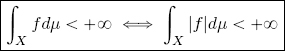
Absolute integrability is a necessary and sufficient condition for integrability of a real or complex valued function:
3.5. Characterization of the Lebesgue measure on ℝ and sets with a null Lebesgue measure
As we have seen, the construction of a measure is generally not trivial. However, given the importance of the Lebesgue measure on ℝ, it is helpful to provide a brief summary of the characteristics of this measure. Remarkably, a theorem exists which provides the characterization of the Lebesgue measure using certain properties. Before quoting the result, we recall some definitions.
– Borel measure: Let X be a topological space, and take the measurable space (X, ![]() (X)), where
(X)), where ![]() (X) is the Borel σ-algebra. A measure μ defined on this space is said to be a Borel measure if it associates a finite number with each compact subset K of X;
(X) is the Borel σ-algebra. A measure μ defined on this space is said to be a Borel measure if it associates a finite number with each compact subset K of X;
– Regular Borel measure: A Borel measure is regular if, for any Borel set E ∈ ![]() (X), we have:
(X), we have:
1) μ(E) = sup{μ(K), K ⊂ E, K compact};
2) μ(E) = inf{μ(O), E ⊂ O, O open}.
Consider now (ℝ, ![]() (ℝ), μ). μ is a shift-invariant measure if:
(ℝ), μ). μ is a shift-invariant measure if:
for any Borel set E ∈ ![]() (ℝ) and all a ∈ ℝ, where E + a = {x ∈ ℝ : x = e + a, where e ∈ E}.
(ℝ) and all a ∈ ℝ, where E + a = {x ∈ ℝ : x = e + a, where e ∈ E}.
We can now quote the theorem that provides the characterization of the Lebesgue measure on ℝ, noted m.
THEOREM 3.2.– If a measure on (ℝ, ![]() (ℝ), μ) has the following properties:
(ℝ), μ) has the following properties:
1) μ is a regular Borel measure;
2) μ is shift-invariant;
3) μ is normalized, that is μ[0, 1] = 1;
then μ is the Lebesgue measure m.
Thus, we can say that the Lebesgue measure on (ℝ, ![]() (ℝ)) is a regular, shift-invariant, normalized Borel measure; this also implies that m[a, b] = b − a.
(ℝ)) is a regular, shift-invariant, normalized Borel measure; this also implies that m[a, b] = b − a.
A further consequence of this theorem is that the Lebesgue measure is σ-finite: ℝ can be covered by a partition of compact intervals [−n, n] with n ∈ ℕ, all of which possess finite measures (μ[−n, n] = 2n).
Generalization of the Lebesgue measure on ℝ to ℝn is straightforward, and we can prove that, if a function is Riemann-integrable on ℝn, it is also Lebesgue-integrable and the two integrals coincide.
Important examples of sets with null Lebesgue measure are given by hypersurfaces of dimension n − 1 in ℝn, such as two-dimensional (2D) surfaces in ℝ3 and curves in ℝ2. Regarding ℝ, since ℝ has the cardinality of continuous, the subsets of ℝ with lower cardinality, that is, countable or finite subsets, have null Lebesgue measure, in particular:
This means that even if we eliminated from a measurable set in ℝ, for example an interval [a, b], a countably infinite number of points, its Lebesgue measure would not change.
This property means that the class of Lebesgue-integrable functions is much broader than that of Riemann-integrable functions. Take the case of a piecewise continuous function on a set with a finite or countable number of jump discontinuities: this function has no Riemann integral. It does, however, have a Lebesgue integral, which is the algebraic sum of the Riemann integrals of each section for which the function is continuous. As the number of discontinuities is finite or countable, we can simply ignore them, since they constitute a set of null Lebesgue measure and therefore have no effect on the final result of integration.
It is important to remember that Lebesgue integration theory does not provide more advanced tools for the explicit calculation of integrals, except in certain very specific cases; however, as just discussed, it allows us to give a meaningful sense to integrals of functions which are much less regular than is required for Riemann integration.
This result, along with the crucial theorems presented in section 3.6, gives Lebesgue integration theory a significant advantage over that of Riemann.
3.6. Three theorems for limit operations in integration theory
In this section, we shall summarize the three most important theorems concerning the limit operation in integration theory. These will be used in Chapter 4.
In these theorems, we shall take (X, ![]() , μ) to be an arbitrary fixed measure space.
, μ) to be an arbitrary fixed measure space.
THEOREM 3.3 (Monotone convergence theorem – Beppo Levi).– Let (fn)n∈ℕ, with fn : X → ℝ, be a monotonically increasing sequence of integrable functions. If the sequence of integrals is bounded, that is:
then ![]() a.e. Furthermore, if we define the limit function f : X → ℝ as:
a.e. Furthermore, if we define the limit function f : X → ℝ as:
then f is integrable, and the limit and integral commute:
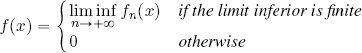
Let us now pass to Fatou’s lemma by first recalling that, given an arbitrary sequence (xn)n∈ℕ of real numbers, lim inf is the limit inferior of the sequence, that is:
THEOREM 3.4 (Fatou’s lemma).– Let (fn)n∈ℕ, with fn : X → ℝ, be a sequence of positive integrable functions and let ![]() . The function f defined by:
. The function f defined by:
is integrable, moreover, the following inequality holds:
THEOREM 3.5 (Dominated convergence theorem – Henri Lebesgue).– Let (fn)n∈ℕ, where fn : X → ℝ, be sequence of measurable functions, and let Φ : X → ℝ be a positive and integrable function such that:
If the real sequence (fn(x))n∈ℕ is convergent ∀x ∈ X and if ![]() then fn and f are integrable and the limit and the integral commute, that is:
then fn and f are integrable and the limit and the integral commute, that is:
3.7. Summary
In this chapter, we provided a brief overview of key elements of measure theory and Lebesgue integration, touching on subjects such as σ-algebra, measurable sets, measures, measure spaces and measurable functions.
Particular attention was paid to the Borel σ-algebra in a topological space: this σ-algebra is generated by the open subsets of the space in question.
Almost-everywhere (a.e.) properties play an important role in measure theory: a property is verified a.e. if it is valid on a measurable subset such that the measure of its complementary set is null.
We saw that the Lebesgue measure m on ℝ can be characterized with respect to the Borel σ-algebra as a regular, normalized and shift-invariant measure. Remarkable examples of null Lebesgue measures in ℝ include countable sets, specifically m(ℕ) = m(ℤ) = m(ℚ) = 0.
Given a measure, the definition of the integral of a measurable function is straightforward and follows a standard approach. We begin by considering simple (or step) functions, which are linear combinations of characteristic functions of measurable sets. Simple functions approach any non-negative measurable function from below. This result is essential, allowing us to define the integral of non-negative measurable functions as the sup of the integral of simple functions which are not greater than the function itself. This definition is extended to arbitrary real-valued functions by using their positive and negative parts, and to complex-valued functions by using their real and imaginary parts.
Finally, we outlined the three fundamental theorems concerning the relation between limits and integrals in Lebesgue theory: the monotonic and dominated convergence theorems (developed by Levi and Lebesgue, respectively) and Fatou’s lemma.