
CHAPTER 8
PHYSICAL DATABASE DESIGN
If computers ran at infinitely fast speeds and data stored on disks could be found and brought into primary memory for processing literally instantly, then logical database design would be the only kind of database design to talk about. Well structured, redundancy-free third normal form tables are the ideal relational database structures and, in a world of infinite speeds, would be practical, too. But, as fast as computers have become, their speeds are certainly not infinite and the time necessary to find data stored on disks and bring it into primary memory for processing are crucial issues in whether an application runs as fast as it must. For example, if you telephone your insurance company to ask about a claim you filed and the customer service agent takes two minutes to find the relevant records in the company's information system, you might well become frustrated with the company and question its ability to handle your business competently. Data storage, retrieval, and processing speeds do matter. Regardless of how elegant an application and its database structures are, if the application runs so slowly that it is unacceptable in the business environment, it will be a failure. This chapter addresses how to take a well structured relational database design and modify it for improved performance.
OBJECTIVES
- Describe the principles of file organizations and access methods.
- Describe how disk storage devices work.
- Describe the concept of physical database design.
- List and describe the inputs to the physical database design process.
- Describe a variety of physical database design techniques ranging from adding indexes to denormalization.
CHAPTER OUTLINE
Introduction
Disk Storage
- The Need for Disk Storage
- How Disk Storage Works
File Organizations and Access Methods
- The Goal: Locating a Record
- The Index
- Hashed Files
Inputs to Physical Database Design
- The Tables Produced by the Logical Database Design Process
- Business Environment Requirements
- Data Characteristics
- Application Characteristics
- Operational Requirements: Data Security, Backup, and Recovery
Physical Database Design Techniques
- Adding External Features
- Reorganizing Stored Data
- Splitting a Table into Multiple Tables
- Changing Attributes in a Table
- Adding Attributes to a Table
- Combining Tables
- Adding New Tables
Example: Good Reading Book Stores
Example: World Music Association
Example: Lucky Rent-A-Car
Summary
INTRODUCTION
Database performance can be adversely affected by a wide variety of factors, as shown in Figure 8.1. Some factors are a result of application requirements and often the most obvious culprit is the need for joins. Joins are an elegant solution to the need for data integration, but they can be unacceptably slow in many cases. Also, the need to calculate and retrieve the same totals of numeric data over and over again can cause performance problems. Another type of factor is very large volumes of data. Data is the lifeblood of an information system, but when there is a lot of it, care must be taken to store and retrieve it efficiently to maintain acceptable performance. Certain factors involving the structure of the data, such as the amount of direct access provided and the presence of clumsy, multi-attribute primary keys, can certainly affect performance. If related data in different tables that must be retrieved together is physically dispersed on the disk, retrieval performance will be slower than if the data is stored physically close together on the disk. Finally, the business environment often presents significant performance challenges. We want data to be shared and to be widely used for the benefit of the business. However, a very large number of access operations to the same data can cause a bottleneck that can ruin the performance of an application environment. And giving people access to more data than they need to see can be a security risk.
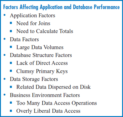
FIGURE 8.1 Factors affecting application and database performance
CONCEPTS IN ACTION
8-A DUCKS UNLIMITED
Ducks Unlimited (“DU”) is the world's largest wetlands conservation organization. It was founded in 1937 when sportsmen realized that they were seeing fewer ducks on their migratory paths and the cause was found to be the destruction of their wetlands breeding areas. Today, with programs reaching from the arctic tundra of Alaska to the tropical wetlands of Mexico, DU is dedicated, in priority order, to preserving existing wetlands, rebuilding former wetlands, and building new wetlands. DU is a non-profit organization headquartered in Memphis, TN, with regional offices located in the four major North American duck “flyways”. DU also works with affiliated organizations in Canada and Mexico to deliver their mutual conservation mission. DU has 600 employees, over 70,000 volunteers, 756,000 paying members, and over one million total contributors. Currently its annual income exceeds $140 million.
In 1999, Ducks Unlimited introduced a major relational database application that it calls its Conservation System, or “Conserv” for short. Located at its Memphis headquarters, Conserv is a project-tracking system that manages both the operational and financial aspects of DU's wetlands conservation projects. In terms of operations, Conserv tracks the phases of each project and the subcontractors performing the work. As for finances, Conserv coordinates the chargeback of subcontractor fees to the “cooperators” (generally federal agencies, landowners, or large contributors) who sponsor the projects.
Conserv is based on the Oracle DBMS and runs on COMPAQ servers. The database has several main tables, including the Project table and the Agreement with cooperators) table, each of which has several subtables. DU employees query the database with Oracle Discoverer to check how much money has been spent on a project and how much of the expenses have been recovered from the cooperators, as two examples. Each night, Conserv sends data to and receives data from a separate relational database running on an IBM AS/400 system that handles membership data, donor history, and accounting functions such as invoicing and accounts payable. Conserv data can even be sent to a geographic information system (GIS) that displays the projects on maps.

Photo Courtesy of Ducks Unlimited
Physical database design is the process of modifying a database structure to improve the performance of the run-time environment. That is, we are going to modify the third normal form tables produced by the logical database design techniques to speed up the applications that will use them. A variety of kinds of modifications can be made, ranging from simply adding indexes to making major changes to the table structures. Some of the changes, while making some applications run faster, may make other applications that share the data run slower. Some of the changes may even compromise the principle of avoiding data redundancy! We will investigate and explain a number of physical database design techniques in this chapter, pointing out the advantages and disadvantages of each.
In order to discuss physical database design, we will begin with a review of disk storage devices, file organizations, and access methods.
DISK STORAGE
The Need for Disk Storage
Computers execute programs and process data in their main or primary memory. Primary memory is very fast and certainly does permit direct access, but it has several drawbacks:
- It is relatively expensive.
- It is not transportable (that is, you can't remove it from the computer and carry it away with you, as you can an external hard drive).
- It is volatile. When you turn the computer off you lose whatever data is stored in it.
Because of these shortcomings, the vast volumes of data and the programs that process them are held on secondary memory devices. Data is loaded from secondary memory into primary memory when required for processing (as are programs when they are to be executed). A loose analogy can be drawn between primary and secondary memory in a computer system and a person's brain and a library, Figure 8.2. The brain cannot possibly hold all of the information a person might need, but (let's say) a large library can. So when a person needs some particular information that's not in her brain at the moment, she finds a book in the library that has the information and, by reading it, transfers the information from the book to her brain. Secondary memory devices in use today include compact disks and magnetic tape, but by far the predominant secondary memory technology in use today is magnetic disk, or simply “disk.”
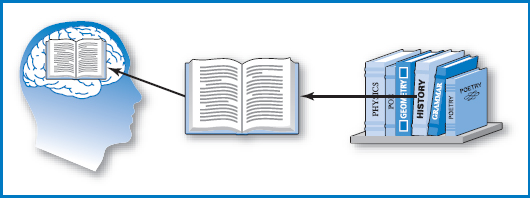
FIGURE 8.2 Primary and secondary memory are like a brain and a library
How Disk Storage Works
The Structure of Disk Devices Disk devices, commonly called “disk drives,” come in a variety of types and capacities ranging from a single aluminum or ceramic disk or “platter” to large multi-platter units that hold many billions of bytes of data. Some disk devices, like “external hard drives,” are designed to be removable and transportable from computer to computer; others, such as the “fixed” or “hard” disk drives in PCs and the disk drives associated with larger computers, are designed to be non-removable. The platters have a metallic coating that can be magnetized and this is how the data is stored, bit by bit. Disks are very fast in storage and retrieval times (although not nearly as fast as primary memory), provide a direct access capability to the data, are less expensive than primary memory units on a byte-by-byte basis, and are non-volatile (when you turn off the computer or unplug the external drive, you don't lose the data on the disk).
It is important to see how data is arranged on disks to understand how they provide a direct access capability. It is also important because certain decisions on how to arrange file or database storage on a disk can seriously affect the performance of the applications using the data.
In the large disk devices used with mainframe computers and midsized “servers” (as well as the hard drives or fixed disks in PCs), several disk platters are stacked together and mounted on a central spindle, with some space between them, Figure 8.3. In common usage, even a multi-platter arrangement like this is simply referred to as “the disk.” Each of the two surfaces of a platter is a recording surface on which data can be stored. (Note: In some of these devices, the upper surface of the topmost platter and the lower surface of the bottommost platter are not used for storing data. We will assume this situation in the following text and figures.) The platter arrangement spins at high speed in the disk drive. The basic disk drive (there are more complex variations) has an “access-arm mechanism” with arms that can reach in between the disks, Figure 8.4. At the end of each arm are two “read/write heads,” one for storing and retrieving data from the recording surface above the arm and the other for the surface below the arm, as shown in the figure. It is important to understand that the entire accessarm mechanism always moves as a unit in and out among the disk platters, so that the read/write heads are always p aligned exactly one above the other in a straight line. The platters spin at high velocity on the central spindle, all together as a single unit. The spinning of the platters and the ability of the access-arm mechanism to move in and out allows the read/write heads to be located over any piece of data on the entire unit, many times each second, and it is this mechanical system that provides the direct access capability.
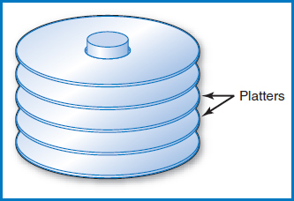
FIGURE 8.3 The platters of a disk are mounted on a central spindle
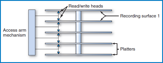
FIGURE 8.4 A disk drive with its access arm mechanism and read/write heads
Tracks On a recording surface, data is stored, serially by bit (bit by bit, byte by byte, field by field, record by record), in concentric circles known as tracks, Figure 8.5. There may be fewer than one hundred or several hundred tracks on each recording surface, depending on the particular device. Typically, each track holds the same amount of data. The tracks on a recording surface are numbered track 0, track 1, track 2, and so on. How would you store the records of a large file on a disk? You might assume that you would fill up the first track on a particular surface, then fill up the next track on the surface, then the next, and so on until you have filled an entire surface. Then you would move on to the next surface. At first, this sounds reasonable and perhaps even obvious. But it turns out it's problematic. Every time you move from one track to the next on a surface, the device's access-arm mechanism has to move. That's the only way that the read/write head, which can read or write only one track at a time, can get from one track to another on a given recording surface. But the access-arm mechanism's movement is a slow, mechanical motion compared to the electronic processing speeds in the computer's CPU and main memory. There is a better way to store the file!
Cylinders Figure 8.6 shows the disk's access-arm mechanism positioned so that the read/write head for recording surface 0 is positioned at that surface's track 76. Since the entire access-arm mechanism moves as a unit and the read/write heads are always one over the other in a line, the read/write head for recording surface 1 is positioned at that surface's track 76, too. In fact, each surface's read/write head is positioned over its track 76. If you picture the collection of each surface's track 76, one above the other, they seem to take the shape of a cylinder, Figure 8.7. Indeed, each collection of tracks, one from each recording surface, one directly above the other, is known as a cylinder. Notice that the number of cylinders in a disk is equal to the number of tracks on any one of its recording surfaces.
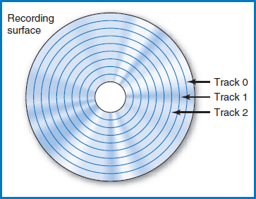
FIGURE 8.5 Tracks on a recording surface
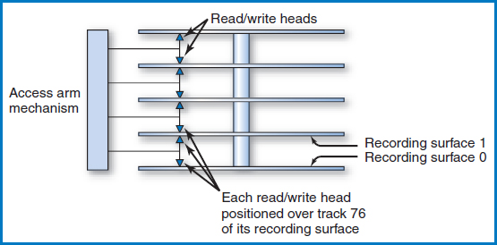
FIGURE 8.6 Each read/write head positioned over track 76 of its recording surface
If we want to number the cylinders in a disk, which seems like a reasonable thing to do, it is certainly convenient to give a cylinder the number corresponding to the track numbers it contains. Thus, the cylinder in Figure 8.7, which is made up of track 76 from each recording surface, will be numbered and called cylinder 76. There is one more point to make. So far, the numbering we have looked at has been the numbering of the tracks on the recording surfaces, which also led to the numbering of the cylinders. But, once we have established a cylinder, it is also necessary to number the tracks within the cylinder, Figure 8.8. Typically, these are numbered 0, 1,…,n, which corresponds to the numbers of the recording surfaces. What will “n” be? That's the same question as how many tracks are there in a cylinder, but we've already answered that question. Since each recording surface “ contributes” one track to each cylinder, the number of tracks in a cylinder is the same as the number of recording surfaces in a disk. The bottom line is to remember that we are going to number the tracks across a recording surface and then, perpendicular to that, we are also going to number the tracks in a cylinder.
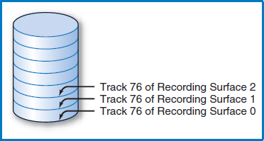
FIGURE 8.7 The collection of each recording surface's track 76 looks like a cylinder. This collection of tracks is called cylinder 76
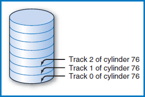
FIGURE 8.8 Cylinder 76's tracks
Why is the concept of the cylinder important? Because in storing or retrieving data on a disk, you can move from one track of a cylinder to another without having to move the access-arm mechanism. The operation of turning off one read/write head and turning on another is an electrical switch that takes almost no time compared to the time it takes to move the access-arm mechanism. Thus, the ideal way to store data on a disk is to fill one cylinder and then move on to the next cylinder, and so on. This speeds up the applications that use the data considerably. Incidentally, it may seem that this is important only when reading files sequentially, as opposed to when performing the more important direct access operations. But we will see later that in many database situations closely related pieces of data will have to be accessed together, so that storing them in such a way that they can be retrieved quickly can be a big advantage.
Steps in Finding and Transferring Data Summarizing the way these disk devices work, there are four major steps or timing considerations in the transfer of data from a disk to primary memory:
- Seek Time: The time it takes to move the access-arm mechanism to the correct cylinder from its current position.
- Head Switching: Selecting the read/write head to access the required track of the cylinder.
- Rotational Delay: Waiting for the desired data on the track to arrive under the read/write head as the disk is spinning. On average, this takes half the time of one full rotation of the disk. That's because, as the disk is spinning, at one extreme the needed data might have just arrived under the read/write head at the instant the head was turned on, while at the other extreme you might have just missed it and have to wait for a full rotation. On the average, this works out to half a rotation.
- Transfer Time: The time to move the data from the disk to primary memory once steps 1–3 have been completed.
One last point. Another term for a record in a file is a logical record. Since the rate of processing data in the CPU is much faster than the rate at which data can be brought in from secondary memory, it is often advisable to transfer several consecutively stored logical records at a time. Once such a physical record or block of several logical records has been brought into primary memory from the disk, each logical record can be examined and processed as necessary by the executing program.
FILE ORGANIZATIONS AND ACCESS METHODS
The Goal: Locating a Record
Depending on application requirements, we might want to retrieve the records of a file on either a sequential or a direct-access basis. Disk devices can store records in some logical sequence, if we wish, and can access records in the middle of a file. But that's still not enough to accomplish direct access. Direct access requires the combination of a direct access device and the proper accompanying software.
Say that a file consists of many thousands or even a few million records. Further, say that there is a single record that you want to retrieve and you know the value of its unique identifier, its key. The question is, how do you know where it is on the disk? The disk device may be capable of going directly into the middle of a file to pull out a record, but how does it know where that particular record is? Remember, what we're trying to avoid is having it read through the file in sequence until it finds the record being sought. It's not magic (nothing in a computer ever is) and it is important to have a basic understanding of each of the steps in working with simple files, including this step, before we talk about databases. This brings us to the subject known as “file organizations and access methods,” which refers to how we store the records of a file on the disk and how we retrieve them. We refer to the way that we store the data for subsequent retrieval as the file organization. The way that we retrieve the data, based on it being stored in a particular file organization, is called the access method. (Note in passing that the terms “file organization” and “access method” are often used synonymously, but this is technically incorrect.)
What we are primarily concerned with is how to achieve direct access to the records of a file, since this is the predominant mode of file operation, today. In terms of file organizations and access methods, there are basically two ways of achieving direct access. One involves the use of a tool known as an “index.” The other is based on a way of storing and retrieving records known as a “hashing method.” The idea is that if we know the value of a field of a record we want to retrieve, the index or hashing method will pinpoint its location in the file and tell the hardware mechanisms of the disk device where to find it.
The Index
The interesting thing about the concept of an index is that, while we are interested in it as a tool for direct access to the records in files, the principle involved is exactly the same as of the index in the back of a book. After all, a book is a storage medium for information about some subject. And, in both books and files, we want to be able to find some portion of the contents “directly” without having to scan sequentially from the beginning of the book or file until we find it. With a book, there are really three choices for finding a particular portion of the contents. One is a sequential scan of every page starting from the beginning of the book and continuing until the desired content is found. The second is using the table of contents. The table of contents in the front of the book summarizes what is in the book by major topics, and it is written in the same order as the material in the book. To use the table of contents, you have to scan through it from the beginning and, because the items it includes are summarized and written at a pretty high level, there is a good chance that you won't find what you're looking for. Even if you do, you will typically be directed to a page in the vicinity of the topic you're looking for, not to the exact page. The third choice is to use the index at the back of the book. The index is arranged alphabetically by item. As humans, we can do a quick, efficient search through the index, using the fact that the items in it are in alphabetic order, to quickly home in on the topic of interest. Then what? Next to the located item in the index appears a page number. Think of the page number as the address of the item you're looking for. In fact, it is a “direct pointer” to the page in the book where the material appears. You proceed directly to that page and find the material there, Figure 8.9.
The index in the back of a book has three key elements that are also characteristic of information systems indexes:
- The items of interest are copied over into the index but the original text is not disturbed in any way.
- The items copied over into the index are sorted (alphabetized in the index at the back of a book).
- Each item in the index is associated with a “pointer” (in a book index this is a page number) pointing to the place in the text where the item can be found.
Simple Linear Index The indexes used in information systems come in a variety of types and styles. We will start with what is called a “simple linear index,” because it is relatively easy to understand and is very close in structure to the index in the back of a book. On the right-hand side of Figure 8.10 is the Salesperson file. As before, it is in order by the unique Salesperson Number field. It is reasonable to assume that the records in this file are stored on the disk in the sequence shown in Figure 8.10. (We note in passing that retrieving the records in physical sequence, as they are stored on the disk, would also be retrieving them in logical sequence by salesperson number, since they were ordered on salesperson number when they were stored.) Figure 8.10 also shows that we have numbered the records of the file with a “Record Number” or a “Relative Record Number” (“relative” because the record number is relative to the beginning of the file). These record numbers are a handy way of referring to the records of the file and using such record numbers is considered another way of “physically” locating a record in a file, just as a cylinder and track address is a physical address.
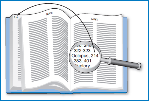
FIGURE 8.9 The index in a book
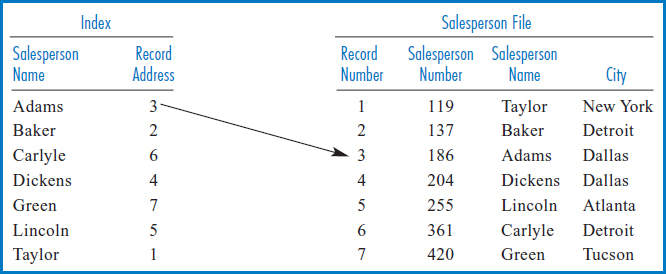
FIGURE 8.10 Salesperson file on the right with index built over the Salesperson Name field, on the left
On the left-hand side of Figure 8.10 is an index built over the Salesperson Name field of the Salesperson file. Notice that the three rules for building an index in a book were observed here, too. The indexed items were copied over from the file to the index and the file was not disturbed in any way. The items in the index were sorted. Finally, each indexed item was associated with a physical address, in this case the relative record number (the equivalent of a page number in a book) of the record of the Salesperson file from which it came. The first “index record” shows Adams 3 because the record of the Salesperson file with salesperson name Adams is at relative record location 3 in the Salesperson file. Notice the similarity between this index and the index in the back of a book. Just as you can quickly find an item you are looking for in a book's index because the items are in alphabetic order, a programmed procedure could quickly find one of the salespersons' names in the index because they are in sorted order. Then, just as the item that you found in the book's index has a page number next to it telling you where to look for the detailed information you seek, the index record in the index of Figure 8.10 has the relative record number of the record of the Salesperson file that has the information, i.e. the record, that you are looking for.
Figure 8.11, with an index built over the City field, demonstrates another point about indexes. An index can be built over a field with non-unique values.
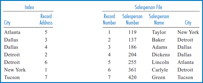
FIGURE 8.11 Salesperson file on the right with index built over the City field, on the left
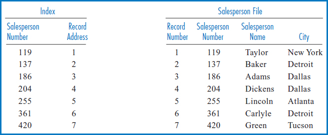
FIGURE 8.12 Salesperson file on the right with index built over the Salesperson Number field, on the left
Figure 8.12 shows the Salesperson file with an index built over the Salesperson Number field. This is an important concept known as an “indexed-sequential file.” In an indexed-sequential file, the file is stored on the disk in order based on a set of field values (in this case the salesperson numbers) and an index is built over that same field. This allows both sequential and direct access by the key field, which can be an advantage when applications with different retrieval requirements share the file. The odd thing about this index is that since the Salesperson file was already in sequence by the Salesperson Number field, when the salesperson numbers were copied over into the index they were already in sorted order! Further, for the same reason, the record addresses are also in order. In fact, in Figure 8.12, the Salesperson Number field in the Salesperson file, with the list of relative record numbers next to it, appears to be identical to the index. But then, why bother having an index built over the Salesperson Number field at all? In principle, the reason is that when the search algorithm processes the salesperson numbers, they have to be in primary memory. Again in principle, it would be much more efficient to bring the smaller index into primary memory for this purpose than to bring the entire Salesperson file in just to process the Salesperson Number field.
Why, in the last couple of sentences, did we keep using the phrase, “in principle?” The answer to this is closely tied to the question of whether simple linear indexes are practical for use in even moderately sized information systems applications. And the answer is that they are not. One reason (and here is where the “in principle” in the last paragraph come in) is that, even if the simple linear index is made up of just two columns, it would still be clumsy to try to move all or even parts of it into primary memory to use it in a search. At best, it would require many read operations to the disk on which the index is located. The second reason has to do with inserting new disk records. Look once again at the Salesperson file and the index in Figure 8.10. Say that a new salesperson named French is hired and assigned salesperson number 452. Her record can be inserted at the end of the Salesperson file, where it would become record number 8. But the index would have to be updated, too: an index record, French 8, would have to be inserted between the index records for Dickens and Green to maintain the crucial alphabetic or sorted sequence of the index, Figure 8.13. The problem is that there is no obvious way to accomplish that insertion unless we move all the index records from Green to Taylor down one record position. In even a moderate-size file, that would clearly be impractical!
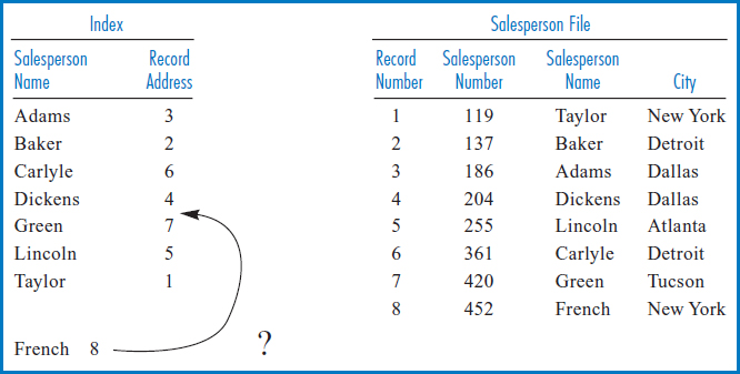
FIGURE 8.13 Salesperson file with the insertion of a record for #452 French. But how can you squeeze the index record into the proper sequence?
Indeed, the simple linear index is not a good solution for indexing the records of a file. This leads us to another kind of index that is suitable for indexing even very large files, the B+−tree index.
B+−Tree Index The B+−tree index, in its many variations (and there are many, including one called the B*-tree), is far and away the most common data-indexing system in use today. Assume that the Salesperson File now includes records for several hundred salespersons. Figure 8.14 is a variation of how the B+−tree index works. The figure shows the salesperson records arranged in sequence by the Salesperson Number field on ten cylinders (numbered 1–10) of a disk. Above the ten cylinders is an arrangement of special index records in what is known as a “tree.” There is a single index record, known as the “root,” at the top, with “branches” leading down from it to other “nodes.” Sometimes the lowest-level nodes are called “leaves.” For the terminology, think of it as a real tree turned upside-down with the roots clumped into a single point at the top, Figure 8.15.
YOUR TURN
8.1 SIMPLE LINEAR INDEXES
When we think of indexes (other than those used to access data in computers), most people would agree that those thoughts would be limited to the indexes in the backs of books. But, if we want to and it makes sense, we can create indexes to help us find objects in our world other than items inside books. (By the way, have you ever seen a directory in a department store that lists its departments alphabetically and then, next to each department name, indicates the floor it's on? That's an index, too!)
QUESTION:
Choose a set of objects in your world and develop a simple linear index to help you find them when you need to. For example, you may have CDs or DVDs on different shelves of a bookcase or in different rooms of your house. In this example, what would be the identifier in the index for each CD or DVD? What would be the physical location in the index? Think of another set of objects and develop an index for them.
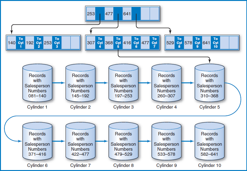
FIGURE 8.14 Salesperson file with a B+−tree index
Alternatively, you can think of it as a family tree, which normally has this same kind of top-to-bottom orientation.
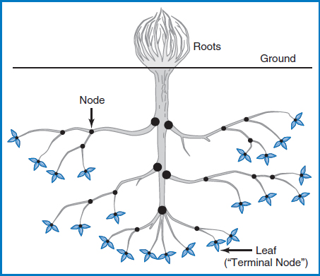
FIGURE 8.15 A real tree, upside down, with the roots clumped together into a single point
Notice the following about the index records in the tree:
- The index records contain salesperson number key values copied from certain of the salesperson records.
- Each key value in the tree is associated with a pointer that is the address of either a lower-level index record or a cylinder containing the salesperson records.
- Each index record, at every level of the tree, contains space for the same number of key value/pointer pairs (four in this example). This index record capacity is arbitrary, but once it is set, it must be the same for every index record at every level of the index.
- Each index record is at least half full (in this example each record actually contains at least two key value/pointer pairs).
How are the key values in the index tree constructed and how are the pointers arranged? The lowest level of the tree contains the highest key value of the salesperson records on each of the 10 data cylinders. That's why there are 10 key values in the lowest level of the index tree. Each of those 10 key values has a pointer to the data cylinder from which it was copied. For example, the leftmost index record on the lowest level of the tree contains key values 140, 192, and 253, which are the highest key values on cylinders 1, 2, and 3, respectively. The root index record contains the highest key value of each of the index records at the next (which happens to be the last in this case) level down. Looking down from the root index record, notice that 253 is the highest key value of the first index record at the next level down, and so on for key values 477 and 641 in the root.
Let's say that you want to perform a direct access for the record for salesperson 361. A stored search routine would start at the root and scan its key values from left to right, looking for the first key value greater than or equal to 361, the key value for which you are searching. Starting from the left, the first key value in the root greater than or equal to 361 is 477. The routine would then follow the pointer associated with key value 477 to the second of the three index records at the next level. The search would be repeated in that index record, following the same rules. This time, key value 368 is the first one from the left that is higher than or equal to 361. The routine would then follow the pointer associated with key value 368 to cylinder 5. Additional search cues within the cylinder could then point to the track and possibly even the position on the track at which the record for salesperson 361 is to be found.
There are several additional points to note about this B+−tree arrangement:
- The tree index is small and can be kept in main memory indefinitely for a frequently accessed file.
- The file and index of Figure 8.14 fit the definition of an indexed-sequential file, because the file is stored in sequence by salesperson numbers and the index is built over the Salesperson Number field.
- The file can be retrieved in sequence by salesperson number by pointing from the end of one cylinder to the beginning of the next, as is typically done, without even using the tree index.
- B+−tree indexes can be and are routinely used to also index non-key, non-unique fields, although the tree can be deeper and/or the structures at the end of the tree can be more complicated.
- In general, the storage unit for groups of records can be (as in the above example) but need not be the cylinder or any other physical device sub-unit.
The final point to make about B+−tree indexes is that, unlike simple linear indexes, they are designed to comfortably handle the insertion of new records into the file and the deletion of records. The principle for this is based on the idea of unit splits and contractions, both at the record storage level and at the index tree level. For example, say that a new record with salesperson number 365 must be inserted. Starting from the root and following the same procedure for a record search, the computer determines that this record should be located on Cylinder 5 in order to maintain the sequence of the records based on the salesperson number key. If there is room on the track on the cylinder that it should go into to maintain the sequence, the other records can be shifted over and there is no problem. If the track it should go into is full but another track on the cylinder has been left empty as a reserve, then the set of records on the full track plus the one for 365 can be “split,” with half of them staying on the original track and the other half moving to the reserve track. There would also have to be a mechanism to maintain the proper sequence of tracks within the cylinder, as the split may have thrown it off.
But suppose that cylinder 5 is completely full. Then the collection of records on the entire cylinder has to be split between cylinder 5 and an empty reserve cylinder, say cylinder 11, Figure 8.16. That's fine, except that the key value of 368 in the tree index's lowest level still points to cylinder 5 while the record with key value 368 is now on cylinder 11. Furthermore, there is no key value/pointer pair representing cylinder 11 in the tree index, at all! If the lowest-level index record containing key value 368 had room, a pointer to the new cylinder could be added and the keys in the key value/pointer pairs adjusted. But, as can be seen in Figure 8.14, there is no room in that index record.
Figure 8.17 shows how this situation is handled. The index record into which the key for the new cylinder should go (the middle of the three index records at the lower level), which happens to be full, is split into two index records. The now five instead of four key values and their associated pointers are divided, as equally as possible, between them. But, in Figure 8.14, there were three key values in the record at the next level up (which happens to be the root), and now there are four index records instead of the previous three at the lower level. As shown in Figure 8.17, the empty space in the root index record is used to accommodate the new fourth index record at the lower level. What would have happened if the root index record had already been full? It would have been split in half and a new root at the next level up would have been created, expanding the index tree from two levels of index records to three levels.
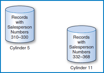
FIGURE 8.16 The records of cylinder 5 plus the newly added record, divided between cylinder 5 and an empty reserve cylinder, cylinder 11
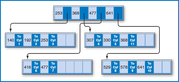
FIGURE 8.17 The B+−tree index after the cylinder 5 split
Remember the following about indexes:
- An index can be built over any field of a file, whether or not the file is in physical sequence based on that or any other field. The field need not have unique values.
- An index can be built on a single field but it can also be built on a combination of fields. For example, an index could be built on the combination of City and State in the Salesperson file.
- In addition to its direct access capability, an index can be used to retrieve the records of a file in logical sequence based on the indexed field. For example, the index in Figure 8.10 could be used to retrieve the records of the Salesperson file in sequence by salesperson name. Since the index is in sequence by salesperson name, a simple scan of the index from beginning to end lists the relative record numbers of the salesperson records in order by salesperson name.
- Many separate indexes into a file can exist simultaneously, each based on a different field or combination of fields of the file. The indexes are quite independent of each other.
- When a new record is inserted into a file, an existing record is deleted, or an indexed field is updated, all of the affected indexes must be updated.
Creating an Index with SQL Creating an index with SQL entails naming the index, specifying the table being indexed, and specifying the column on which the index is being created. So, for example, to create index A in Figure 8.21, which is an index built on the Salesperson Number attribute of the SALESPERSON table, you would write:
CREATE INDEX A ON SALESPERSON(SPNUM);
Hashed Files
There are many applications in which all file accesses must be done on a direct basis, speed is of the essence, and there is no particular need for the file to be organized in sequence by the values of any of its fields. An approach to file organization and access that fills this bill is the hashed file. The basic ideas include:
- The number of records in a file is estimated and enough space is reserved on a disk to hold them.
- Additional space is reserved for additional “overflow” records.
- To determine where to insert a particular record of the file, the record's key value is converted by a “hashing routine” into one of the reserved record locations on the disk.
- To subsequently find and retrieve the record, the same hashing routine is applied to the key value during the search.
Say, for example, that our company has 50 salespersons and that we have reserved enough space on the disk for their 50 records. There are many hashing routines but the most common is the “division-remainder method.” In the division-remainder method, we divide the key value of the record that we want to insert or retrieve by the number of record locations that we have reserved. Remember long division, with its “quotient” and “remainder?” We perform the division, discard the quotient, and use the remainder to tell us where to locate the record. Why the remainder? Because the remainder is tailor-made for pointing to one of the storage locations. If, as in this example, we have 50 storage locations and divide a key value by that number, 50, we will get a remainder that is a whole number between 0 and 49. The value of the quotient doesn't matter. If we number the 50 storage locations 0–49 and store a record at the location dictated by its “hashed” key value, we have clearly developed a way to store and then locate the records, and a very fast way, at that! There's only one problem. More than one key value can hash to the same location. When this happens, we say that a “collision” has occurred, and the two key values involved are known as “synonyms.”
Figure 8.18 shows a storage area that can hold 50 salesperson records plus space for overflow records. (We will not go into how to map this space onto the cylinders and tracks of a disk, but it can be done easily.) The main record storage locations are numbered 0–49; the overflow locations begin at position 50. An additional field for a “synonym pointer” has been added to every record location. Let's start by storing the record for salesperson 186. Dividing 186 by the number of record locations (50) yields a quotient of 3 (which we don't care about) and a remainder of 36. So, as shown in the figure, we store the record for salesperson 186 at record location 36. Next, we want to store the record for salesperson 361. This time, the hashing routine gives a remainder of 11 and, as shown in the figure, that's where the record goes. The next record to be stored is the record for salesperson 436. The hashing routine produces a remainder of 36. The procedure tries to store the record at location 36, but finds that another record is already stored there.
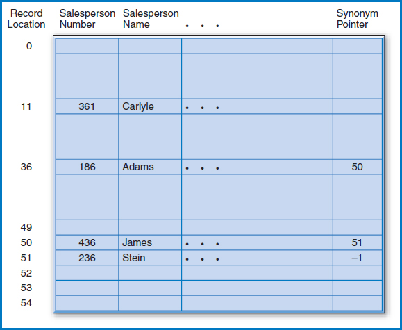
FIGURE 8.18 The Salesperson file stored as a hashed file
To solve this problem, the procedure stores the new record at one of the overflow record locations, say number 50. It then indicates this by storing that location number in the synonym pointer field of record 36. When another collision occurs with the insertion of salesperson 236, this record is stored at the next overflow location and its location is stored at location 50, the location of the last record that “hashed” to 36.
Subsequently, if an attempt is made to retrieve the record for salesperson 186, the key value hashes to 36 and, indeed, the record for salesperson 186 is found at location 36. If an attempt is made to retrieve the record for salesperson 436, the key hashes to 36 but another record (the one for salesperson 186) is found at location 36. The procedure then follows the synonym pointer at the end of location 36 to location 50, where it finds the record for salesperson 436. A search for salesperson 236's record would follow the same sequence. Key value 236 would hash to location 36 but another record would be found there. The synonym pointer in the record at location 36 points to location 50, but another record, 436, is found there, too. The synonym pointer in the record at location 50 points to location 51, where the desired record is found.
There are a few other points to make about hashed files:
- It should be clear that the way that the hashing algorithm scatters records within the storage space disallows any sequential storage based on a set of field values.
- A file can only be hashed once, based on the values of a single field or a single combination of fields. This is because the essence of the hashing concept includes the physical placement of the records based on the result of the hashing routine. A record can't be located in one place based on the hash of one field and at the same time be placed somewhere else based on the hash of another field. It can't be in two places at once!
- If a file is hashed on one field, direct access based on another field can be achieved by building an index on the other field.
- Many hashing routines have been developed. The goal is to minimize the number of collisions and synonyms, since these can obviously slow down retrieval performance. In practice, several hashing routines are tested on a file to determine the best “fit.” Even a relatively simple procedure like the division-remainder method can be fine-tuned. In this method, experience has shown that once the number of storage locations has been determined, it is better to choose a slightly higher number, specifically the next prime number or the next number not evenly divisible by any number less than 20.
- A hashed file must occasionally be reorganized after so many collisions have occurred that performance is degraded to an unacceptable level. A new storage area with a new number of storage locations is chosen and the process starts all over again.
- Figure 8.18 shows a value of –1 in the synonym pointer field of the record for salesperson 236 at storage location 51. This is an end-of-chain marker. It is certainly possible that a search could be conducted for a record, say with key value 386, that does not exist in the file. 386 would hash to 36 and the chain would be followed to location 50 and then to location 51. Some signal has to then be set up at the end of the chain to indicate that there are no more records stored in the file that hash to 36, so that the search can be declared over and a “not found” condition indicated. (A negative number is a viable signal because there can't be a negative record location!)
INPUTS TO PHYSICAL DATABASE DESIGN
Physical database design starts where logical database design ends. That is, the well structured relational tables produced by the conversion from entity-relationship diagrams or by the data normalization process form the starting point for physical database design. But these tables are only part of the story. In order to determine how best to modify the tables to improve application performance, a wide range of factors must be considered. The factors will help determine which modification techniques to apply and how to apply them. And, at that, the process is as much art as science. The choices are so numerous and the possible combinations of modifications are so complex that even the experienced designer hopes for a satisfactory but not a perfect solution.
Figure 8.19 lists the inputs to physical database design and thus the factors that are important to it. These naturally fall into several subgroups. First, we will take a look at each of these physical design inputs and factors, one by one. Then we will describe a variety of physical database design techniques, explaining how the various inputs and factors influence each of these techniques.
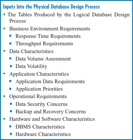
FIGURE 8.19 Inputs into the physical database design process
The Tables Produced by the Logical Database Design Process
The tables produced by the logical database design process (which for simplicity we will refer to as the “logical design”) form the starting point of the physical database design process. These tables are “pure” in that they reflect all of the data in the business environment, they have no data redundancy, and they have in place all the foreign keys that are needed to establish all the relationships in the business environment. Unfortunately, they may present a variety of problems when it comes to performance, as we previously described. Again, for example, without indexes or hashing, there is no support for direct access. Or it is entirely possible that a particular query may require the join of several tables, which may cause an unacceptably slow response from the database. So, it is clear that these tables, in their current form, are very likely to produce unacceptable performance and that is why we must go on modifying them in physical database design.
Business Environment Requirements
Beyond the logical design, the requirements of the business environment lead the list of inputs and factors in physical database design. These include response time requirements and throughput requirements.
Response Time Requirements Response time is the delay from the time that the Enter Key is pressed to execute a query until the result appears on the screen. One of the main factors in deciding how extensively to modify the logical design is the establishment of the response time requirements. Do the major applications that will use the database require two-second response, five-second response, ten-second response, etc.? That is, how long a delay will a customer telephoning your customer service representatives tolerate when asking a question about her account? How fast a response do the managers in your company expect when looking for information about a customer or the sales results for a particular store or the progress of goods on an assembly line? Also, different types of applications differ dramatically in response time requirements. Operational environments, including the customer service example, tend to require very fast response. “Decision support” environments, such as the data warehouse environment discussed in Chapter 13 tend to have relaxed response time requirements.
Throughput Requirements Throughput is the measure of how many queries from simultaneous users must be satisfied in a given period of time by the application set and the database that supports it. Clearly, throughput and response time are linked. The more people who want access to the same data at the same time, the more pressure on the system to keep the response time from dropping to an unacceptable level. And the more potential pressure there is on response time, the more important the physical design task becomes.
Data Characteristics
How much data will be stored in the database and how frequently different parts of it will be updated are important in physical design as well.
Data Volume Assessment How much data will be in the database? Roughly, how many records is each table expected to have? Some physical design decisions will hinge on whether a table is expected to have 300, 30,000, or 3,000,000 records.
Data Volatility Data volatility describes how often stored data is updated. Some data, such as active inventory records that reflect the changes in goods constantly being put into and taken out of inventory, is updated frequently. Some data, such as historic sales records, is never updated (except for the addition of data from the latest time period to the end of the table). How frequently data is updated, the volatility of the data, is an important factor in certain physical design decisions.
Application Characteristics
The nature of the applications that will use the data, which applications are the most important to the company, and which data will be accessed by each application form yet another set of inputs and factors in physical design.
Application Data Requirements Exactly which database tables does each application require for its processing? Do the applications require that tables be joined? How many applications and which specific applications will share particular database tables? Are the applications that use a particular table run frequently or infrequently? Questions like these yield one indication of how much demand there will be for access to each table and its data. More heavily used tables and tables frequently involved in joins require particular attention in the physical design process.
Application Priorities Typically, tables in a database will be shared by different applications. Sometimes, a modification to a table during physical design that's proposed to help the performance of one application hinders the performance of another application. When a conflict like that arises, it's important to know which of the two applications is the more critical to the company. Sometimes this can be determined on an increased profit or cost-saving basis. Sometimes it can be based on which application's sponsor has greater political power in the company. But, whatever the basis, it is important to note the relative priority of the company's applications for physical design choice considerations.
Operational Requirements: Data Security, Backup, and Recovery
Certain physical design decisions can depend on such data management issues as data security and backup and recovery. Data security, which will be discussed in Chapter 11, can include such concerns as protecting data from theft or malicious destruction and making sure that sensitive data is accessible only to those employees of the company who have a “need to know.” Backup and recovery, which will also be discussed in Chapter 11, ranges from recovering a table or a database that has been corrupted or lost due to hardware or software failure to recovering an entire information system after a natural disaster. Sometimes, data security and backup and recovery concerns can affect physical design decisions.
Hardware and Software Characteristics Finally, the hardware and software environments in which the databases will reside have an important bearing on physical design.
YOUR TURN
8.2 PHYSICAL DATABASE DESIGN INPUT
Consider a university information systems environment or another information systems environment of your choice. Think about a set of 5–10 applications that constitute the main applications in this environment.
QUESTION:
For each of these 5–10 applications, specify the response time requirements and the throughput requirements. What would the volumes be of the database tables needed to support these applications? How volatile would you expect the data to be? What concerns would you have about the security and privacy of the data?
DBMS Characteristics All relational database management systems are certainly similar in that they support the basic, even classic at this point, relational model. However, relational DBMSs may differ in certain details, such as the exact nature of their indexes, attribute data type options, SQL query features, etc., that must be known and taken into account during physical database design.
Hardware Characteristics Certain hardware characteristics, such as processor speeds and disk data transfer rates, while not directly parts of the physical database design process, are associated with it. Simply put, the faster the hardware, the more tolerant the system can be of a physical design that avoids relatively severe changes in the logical design.
PHYSICAL DATABASE DESIGN TECHNIQUES
Figure 8.20 lists several physical database design categories and techniques within each. The order of the categories is significant. Depending on how we modify the logical design to try to make performance improvements, we may wind up introducing new complications or even reintroducing data redundancy. Also, as noted in Figure 8.20, the first three categories do not change the logical design while the last four categories do. So, the order of the categories is roughly from least to most disruptive of the original logical design. And, in this spirit, the only techniques that introduce data redundancy (storing derived data, denormalization, duplicating tables, and adding subset tables) appear at the latter part of the list.
Adding External Features
This first category of physical design changes, adding external features, doesn't change the logical design at all! Instead, it involves adding features to the logical design, specifically indexes and views. While certain tradeoffs have to be kept in mind when adding these external features, there is no introduction of data redundancy.
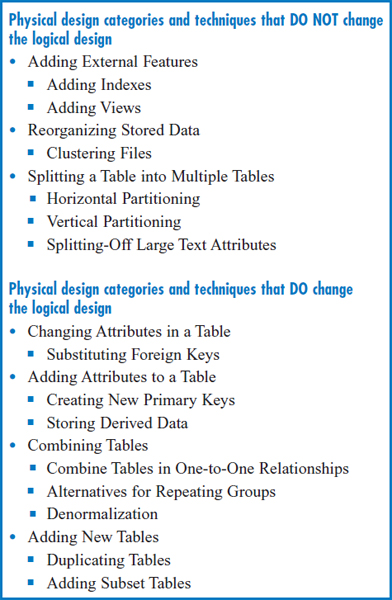
FIGURE 8.20 Physical database design categories and techniques
Adding Indexes Since the name of the game is performance and since today's business environment is addicted to finding data on a direct-access basis, the use of indexes in relational databases is a natural. There are two questions to consider.
The first question is: which attributes or combinations of attributes should you consider indexing in order to have the greatest positive impact on the application environment? Actually, there are two sorts of possibilities. One category is attributes that are likely to be prominent in direct searches. These include:
- Primary keys.
- Search attributes, i.e. attributes whose values you will use to retrieve particular records. This is true especially when the attribute can take on many different values. (In fact, there is an argument that says that it is not beneficial to build an index on an attribute that has only a small number of possible values.)
The other category is attributes that are likely to be major players in operations such as joins that will require direct searches internally. Such operations also include the SQL ORDER BY and GROUP BY commands described in Chapter 4. It should be clear that a particular attribute might fall into both of these categories!
The second question is: what potential problems can be caused by building too many indexes? If it were not for the fact that building too many indexes can cause problems in certain kinds of databases, the temptation would be to build a large number of indexes for maximum direct-access benefit. The issue here is the volatility of the data. Indexes are wonderful for direct searches. But when the data in a table is updated, the system must take the time to update the table's indexes, too. It will do this automatically, but it takes time. If several indexes must be updated, this multiplies the time to update the table several times over. What's wrong with that? If there is a lot of update activity, the time that it takes to make the updates and update all the indexes could slow down the operations that are just trying to read the data for query applications, degrading query response time down to an unacceptable level!
One final point about building indexes: if the data volume, the number of records in a table, is very small, then there is no point in building any indexes on it at all (although some DBMSs will always require an index on the primary key). The point is that if the table is small enough, it is more efficient to just read the whole table into main memory and search by scanning it!
Figure 8.21 repeats the General Hardware Co. relational database, to which we will add some indexes. We start by building indexes, marked indexes A-F, on the primary key attribute(s) of each table. Consider the SALESPERSON and CUSTOMER tables. If the application set requires joins of the SALESPERSON and CUSTOMER tables, the Salesperson Number attribute of the CUSTOMER table would be a good choice for an index, index G, because it is the foreign key that connects those two tables in the join. If we frequently need to find salesperson records on a direct basis by Salesperson Name, then that attribute should have an index, index H, built on it. Consider the SALES table. If we have an important, frequently run application that has to find the total sales for all or a range of the products, then the needed GROUP BY command would run more efficiently if the Product Number attribute was indexed, index I.
Adding Views Another external feature that doesn't change the logical design is the view. In relational database terminology, a view is what is more generally known in database management as a “logical view.” It is a mapping onto a physical table that allows an end user to access only part of the table. The view can include a subset of the table's columns, a subset of the table's rows, or a combination of the two. It can even be based on the join of two tables No data is physically duplicated when a view is created. It is literally a way of viewing just part of a table. For example, in the General Hardware Co. SALESPERSON table, a view can be created that includes only the Salesperson Number, Salesperson Name, and Office Number attributes. A particular person can be given access to the view and then sees only these three columns. He is not even aware of the existence of the other two attributes of the physical table.
A view is an important device in protecting the security and privacy of data, an issue that we listed among the factors in physical database design. Using views to limit the access of individuals to only the parts of a table that they really need to do their work is clearly an important means of protecting a company's data. As we will see later, the combination of the view capability and the SQL GRANT command forms a powerful data protection tool.
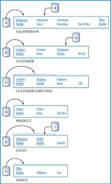
FIGURE 8.21 The General Hardware Company relational database with some indexes
Reorganizing Stored Data
The next level of change in physical design involves reorganizing the way data is stored on the disk without changing the logical design at all and thus without introducing data redundancy. We present an example of this type of modification.
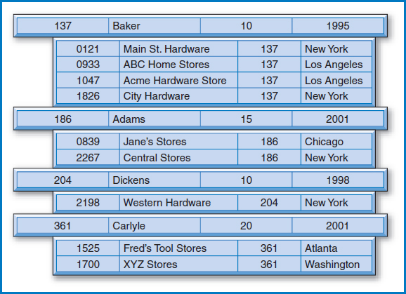
FIGURE 8.22 Clustering files with the SALESPERSON and CUSTOMER tables
Clustering Files Suppose that in the General Hardware Co. business environment, it is important to be able to frequently and quickly retrieve all of the data in a salesperson record together with all of the records of the customers for which that salesperson is responsible. Clearly, this requires a join of the SALESPERSON and CUSTOMER tables. Just for the sake of argument, assume that this retrieval, including the join, does not work quickly enough to satisfy the response time or throughput requirements. One solution, assuming that the DBMS in use supports it, might be the use of “clustered files.”
Figure 8.22 shows the General Hardware salesperson and customer data from Figure 5.14 arranged as clustered files. The logical design has not changed. Logically, the DBMS considers the SALESPERSON and CUSTOMER tables just as they appear in Figure 5.14. But physically, they have been arranged on the disk in the interleaved fashion shown in Figure 8.22. Each salesperson record is followed physically on the disk by the customer records with which it is associated. That is, each salesperson record is followed on the disk by the records of the customers for whom that salesperson is responsible. For example, the salesperson record for salesperson 137, Baker, is followed on the disk by the customer records for customers 0121, 0933, 1047, and 1826. Note that the salesperson number 137 appears as a foreign key in each of those four customer records. So, if a query is posed to find a salesperson record, say Baker 's record, and all his associated customer records, performance will be improved because all five records are right near each other on the disk, even though logically they come from two separate tables. Without the clustered files, Baker's record would be on one part of the disk with all of the other salesperson records and the four customer records would be on another part of the disk with the other customer records, resulting in slower retrieval for this kind of two-table, integrated query.
The downside of this clustering arrangement is that retrieving subsets of only salesperson records or only customer records is slower than without clustering. Without clustering, all the salesperson records are near each other on the disk, which helps when retrieving subsets of them. With clustering, the salesperson records are scattered over a much larger area on the disk because they're interspersed with all of those customer records, slowing down the retrieval of subsets of just salesperson records.
Splitting a Table into Multiple Tables
The three physical design techniques in this category arrange for particular parts of a table, either groups of particular rows or groups of particular columns, to be stored separately, on different areas of a disk or on different disks. In Chapter 12, when we discuss distributed database, we will see that this concept can even be extended to storing particular parts of a table in different cities.
Horizontal Partitioning In horizontal partitioning, the rows of a table are divided into groups and the groups are stored separately, on different areas of a disk or on different disks. This may be done for several reasons. One is to manage the different groups of records separately for security or backup and recovery purposes. Another is to improve data retrieval performance when, for example, one group of records is accessed much more frequently than other records in the table. For example, suppose that the records for sales managers in the CUSTOMER EMPLOYEE table of Figure 5.14c must be accessed more frequently than the records of other customer employees. Separating out the frequently accessed group of records, as shown in Figure 8.23, means that they can be stored near each other in a concentrated space on the disk, which will speed up their retrieval. The records can also be stored on an otherwise infrequently used disk, so that the applications that use them don't have to compete excessively with other applications that need data on the same disk. The downside of this horizontal partitioning is that it can make a search of the entire table or the retrieval of records from more than one partition more complex and slower.
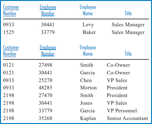
FIGURE 8.23 Horizontal partitioning of the CUSTOMER EMPLOYEE table
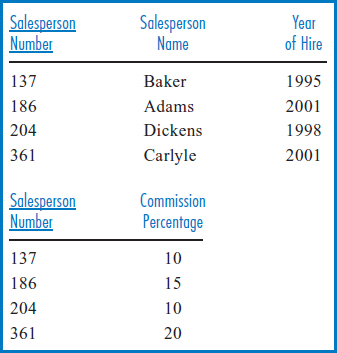
FIGURE 8.24 Vertical partitioning of the SALESPERSON table
Vertical Partitioning A table can also be subdivided by columns, producing the same advantages as horizontal partitioning. In this case, the separate groups, each made up of different columns of a table, are created because different users or applications require different columns. For example, as shown in Figure 8.24, it might be beneficial to split up the columns of the SALESPERSON table of Figure 5.14a so that the Salesperson Name and Year of Hire columns are stored separately from the others. But note that in creating these vertical partitions, each partition must have a copy of the primary key, Salesperson Number in this example. Otherwise, in vertical partitioning, how would you track which rows in each partition go together to logically form the rows of the original table? In fact, this point leads to an understanding of the downside of vertical partitioning. A query that involves the retrieval of complete records—i.e., data that is in more than one vertical partition—actually requires that the vertical partitions be joined to reunite the different parts of the original records.
Splitting Off Large Text Attributes A variation on vertical partitioning involves splitting off large text attributes into separate partitions. Sometimes the records of a table have several numeric attributes and a long text attribute that provides a description of the data in each record. It might well be that frequent access of the numeric data is necessary and that the long text attribute is accessed only occasionally. The problem is that the presence of the long text attribute tends to spread the numeric data over a larger disk area and thus slows down retrieval of the numeric data. The solution is to split off the text attribute, together with a copy of the primary key, into a separate vertical partition and store it elsewhere on the disk.
Changing Attributes in a Table
Up to this point, none of the physical design techniques discussed have changed the logical design. They have all involved adding external features such as indexes and views, or physically moving records or columns on the disk as with clustering and partitioning. The first physical design technique category that changes the logical design involves substituting a different attribute for a foreign key.
Substituting Foreign Keys Consider the SALESPERSON and CUSTOMER tables of Figure 8.21. We know that Salesperson Number is a unique attribute and serves as the primary key of the SALESPERSON table. Say, for the sake of argument, that the Salesperson Name attribute is also unique, meaning that both Salesperson Number and Salesperson Name are candidate keys of the SALESPERSON table. Salesperson Number has been chosen to be the primary key and Salesperson Name is an alternate key.
Now, assume that there is a frequent need to retrieve data about customers, including the name of the salesperson responsible for that customer. The CUSTOMER table contains the number of the Salesperson who is responsible for a customer but not the name. By now, we know that solving this problem requires a join of the two tables, based on the common Salesperson Number attribute. But, if this is a frequent or critical query that requires high speed, we can improve the performance by substituting Salesperson Name for Salesperson Number as the foreign key in the CUSTOMER table, as shown in Figure 8.25. With Salesperson Name now contained in the CUSTOMER table, we can retrieve customer data, including the name of the responsible salesperson, without having to do a performance-slowing join. Finally, since Salesperson Name is a candidate key of the SALESPERSON table, using it as a foreign key in the CUSTOMER table still retains the ability to join the two tables when this is required for other queries.
Adding Attributes to a Table
Another means of improving database performance entails modifying the logical design by adding attributes to tables. Here are two ways to do this.
Creating New Primary Keys Sometimes a table simply does not have a single unique attribute that can serve as its primary key. A two-attribute primary key, such as the combination of state and city names, might be OK. But in some circumstances the primary key of a table might consist of two, three, or more attributes and the performance implications of this may well be unacceptable. For one thing, indexing a multi-attribute key would likely be clumsy and slow. For another, having to use the multi-attribute key as a foreign key in the other tables in which such a foreign key would be necessary would probably also be unacceptably complex.
The solution is to invent a new primary key for the table that consists of a single new attribute. The new attribute will be a unique serial number attribute, with an arbitrary unique value assigned to each record of the table. This new attribute will then also be used as the foreign key in the other tables in which such a foreign key is required. In the General Hardware database of Figure 8.21, recall that the two-attribute primary key of the CUSTOMER EMPLOYEE table, Customer Number and Employee Number, is necessary because customer numbers are unique only within each customer company. Suppose that General Hardware decides to invent a new attribute, Customer Employee Number, which will be its own set of employee numbers for these people that will be unique across all of the customer companies. Then, the current two-attribute primary key of the CUSTOMER EMPLOYEE table can be replaced by this one new attribute, as shown in Figure 8.26. If the Customer Number, Employee Number combination had been placed in other tables in the database as a foreign key (it wasn't), then the two-attribute combination would be replaced by this new single attribute, too. Notice that Customer Number is still necessary as a foreign key because that's how we know which customer company a person works for. Arguably, the old Employee Number attribute may still be required because that is still their employer's internal identifier for them.
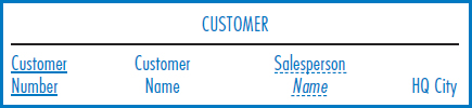
FIGURE 8.25 Substituting another candidate key for a foreign key
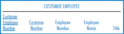
FIGURE 8.26 Creating a new primary key attribute to replace a multiattribute primary key
Storing Derived Data Some queries require performing calculations on the data in the database and returning the calculated values as the answers. If these same values have to be calculated over and over again, perhaps by one person or perhaps by many people, then it might make sense to calculate them once and store them in the database. Technically, this is a form of data redundancy, although a rather subtle form. If the “raw” data is ever updated without the stored, calculated values being updated as well, the accuracy or integrity of the database will be compromised.
To illustrate this point, let's add another attribute to General Hardware's CUSTOMER table. This attribute, called Annual Purchases in Figure 8.27a, is the expected amount of merchandise, in dollars, that a customer will purchase from General Hardware in a year. Remember that there is a one-to-many relationship from salespersons to customers, with each salesperson being responsible for several (or many) customers. Suppose that there is a frequent need to quickly find the total amount of merchandise each salesperson is expected to account for in a year, i.e. the sum of the Annual Purchases attribute for all of the particular salesperson's customers. This sum could be recalculated each time it is requested for any particular salesperson, but that might take too long. The other choice is to calculate the sum for each salesperson and store it in the database, recognizing that whenever a customer's Annual Purchases value changes, the sum for the customer's salesperson has to be updated, too.
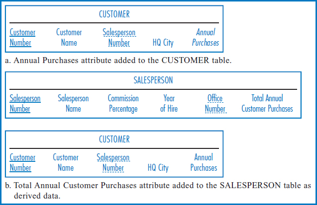
FIGURE 8.27 Adding derived data
The question then becomes, where do we store the summed annual purchases amount for each salesperson? Since the annual purchases figures are in the CUSTOMER table, your instinct might be to store the sums there. But where in the CUSTOMER table? You can't store them in individual customer records, because each sum involves several customers. You could insert special “sum records” in the CUSTOMER table but they wouldn't have the same attributes as the customer records themselves and that would be very troublesome. Actually, the answer is to store them in the SALESPERSON table. Why? Because there is one sum for each salesperson—again, it's the sum of the annual purchases of all of that salesperson's customers. So, the way to do it is to add an additional attribute, the Total Annual Customer Purchases attribute, to the SALESPERSON table, as shown in Figure 8.27b.
Combining Tables
Three techniques are described below, all of which involve combining two tables into one. Each technique is used in a different set of circumstances. It should be clear that all three share the same advantage: if two tables are combined into one, then there must surely be situations in which the presence of the new single table lets us avoid joins that would have been necessary when there were two tables. Avoiding joins is generally a plus for performance. But at what price? Let's see.
Combine Tables in One-to-One Relationships Remember the one-to-one relationship between salespersons and offices in the General Hardware environment? Figure 8.28 shows the two tables combined into one. After all, if a salesperson can have only one office and an office can have only one salesperson assigned to it, there can be nothing wrong with combining the two tables. Since a salesperson can have only one office, a salesperson can be associated with only one office number, one (office) telephone, and one (office) size. A like argument can be made from the perspective of an office. Office data can still be accessed on a direct basis by simply creating an index on the Office Number attribute in the combined table.
Again, the advantage is that if we ever have to retrieve detailed data about a salesperson and his office in one query, it can now be done without a join. There are two negatives. One is that the tables are no longer logically, as well as physically, independent. If we want information just about offices, there is no longer an OFFICE table to go to. The data is still there, but we have to be aware that it is buried in the SALESPERSON/OFFICE table. The other negative is that retrievals of salesperson data alone or of office data alone could be slower than before because the longer combined SALESPERSON/OFFICE records spread the combined data over a larger area of the disk.
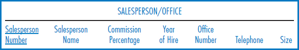
FIGURE 8.28 Combined SALESPERSON/OFFICE table showing the merger of two tables in a one-to-one relationship
Alternatives for Repeating Groups Suppose that we change the business environment so that every salesperson has exactly two customers, identified respectively as their “large” customer and their “small” customer, based on annual purchases. The structure of Figure 8.21 would still work just fine. But, because these “repeating groups” of customer attributes, one “group” of attributes (Customer Number, Customer Name, etc.) for each customer are so well controlled they can be folded into the SALESPERSON table. What makes them so well controlled is that there are exactly two for each salesperson and they can even be distinguished from each other as “large” and “small.” This arrangement is shown in Figure 8.29. Note that the foreign key attribute of Salesperson Number from the CUSTOMER table is no longer needed.
Once again, this arrangement avoids joins when salesperson and customer data must be retrieved together. But, as with the one-to-one relationship case above, retrievals of salesperson data alone or of customer data alone could be slower than before because the longer combined SALESPERSON/CUSTOMER records spread the combined data over a larger area of the disk. And retrieving customer data alone is now more difficult. In the one-to-one relationship case, we could simply create an index on the Office Number attribute of the combined table. But in the combined table of Figure 8.29, there are two customer number attributes in each salesperson record. Retrieving records about customers alone would clearly take greater skill than before.
Denormalization In the most serious database performance dilemmas, when everything else that can be done in terms of physical design has been done, it may be necessary to take pairs of related third normal form tables, and combine them, introducing possibly massive data redundancy. Why would anyone in their right mind want to do this? Because if after everything else has been done to improve performance, response times and throughput are still unsatisfactory for the business environment, eliminating run-time joins by recombining tables may mean the difference between a usable system and a lot of wasted money on a database (and application) development project that will never see the light of day. Clearly, if the physical designers decide to go this route, they must put procedures in place to manage the redundant data as they updated over time.
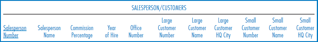
FIGURE 8.29 Merging of repeating groups into another table
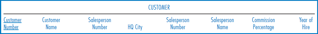
FIGURE 8.30 The denormalized SALESPERSON and CUSTOMER tables as the new CUSTOMER table
Figure 8.30 shows the denormalized SALESPERSON and CUSTOMER tables combined into one. The surviving table of the two in the one-to-many relationship will always be the table on the “many side” of the relationship. You can attach one set of salesperson data to a customer record; you cannot attach many sets of customer data to a single salesperson record without creating an even worse mess. The sample salesperson and customer data from Figure 5.14 is denormalized in Figure 8.31. (Figure 8.31 is identical to Figure 3.8. We used it in Chapter 3 to make a point about data redundancy when we were exploring that subject.) Since a salesperson can have several customers, a particular salesperson's data will be repeated for each customer he has. Thus, the table shows that salesperson number L37's name is Baker four times, his commission percentage is 10 four times, and his year of hire was 1995 four times. The performance improvement had better be worth it, because the integrity exposure is definitely there.
Adding New Tables
Finally, there is the concept of simply duplicating data. Sometimes the final performance issue is that trying to maintain response time and throughput with the number of applications and users trying to share the same data is beyond the capabilities of the hardware, the software, and all the other physical design techniques. At the risk of overt data redundancy (which hopefully you will attempt to managed), the only recourse is to duplicate the data.
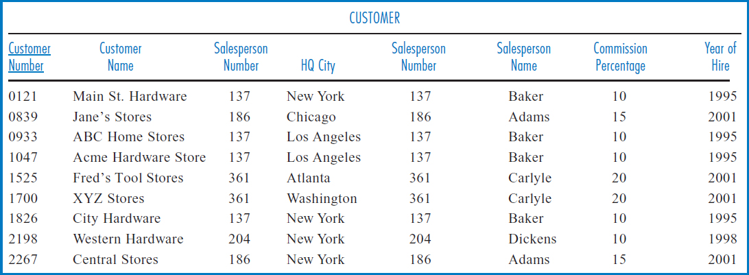
FIGURE 8.31 The denormalized salesperson and customer data from Figure 5.12
Duplicating Tables Clearly, the direct approach is to duplicate tables and have different applications access the duplicates. This is exactly the opposite of the central database management concept of sharing data.
Adding Subset Tables A somewhat less severe technique is to duplicate only those portions of a table that are most heavily accessed. These “subset” tables can then be assigned to different applications to ease the performance crunch. Data redundancy is still the major drawback, although obviously there is not as much of it as when the entire table is duplicated.
EXAMPLE: GOOD READING BOOK STORES
Consider the Good Reading Book Stores database of Figure 5.16. Recall that there is a one-to-many relationship between the PUBLISHER and BOOK tables. A book is published by exactly one publisher but a publisher publishes many books. That's why the Publisher Name attribute is in the BOOK table as a foreign key. A reasonable assumption is that there are several hundred publishers and many thousands of different books. If the various stores in the Good Reading chain carry different books to satisfy their individual clienteles, then there could be thousands of publishers and hundreds of thousands of different books.
Assume that at Good Reading's headquarters, there is a frequent need to find very quickly the details of a book, based on either its book number or its title, together with details about its publisher. As stated, this would clearly require a join of the PUBLISHER and BOOK tables. If the join takes too long, resulting in unacceptable response times, throughput, or both, what are the possibilities in terms of physical design to improve the situation? Here are several suggestions, although each has its potential drawbacks, as previously discussed.
- The Book Number attribute and the Book Title attributes in the PUBLISHER table can each have an index built on them to provide direct access, since the problem says that books are going to be searched for based on one of these two attributes.
- The two join attributes, the Publisher Name attribute of the PUBLISHER table and the Publisher Name attribute of the BOOK table, can each have an index built on them to help speed up the joint operation.
- If the DBMS permits it, the two tables can be clustered, with the book records associated with a particular publisher stored near that publisher's record on the disk.
- The two tables can be denormalized, with the appropriate publisher data being appended to each book record (and the PUBLISHER table being eliminated), as:

What if it's important to be able to find quickly the number of different books that Good Reading carries from a particular publisher? This information could be found by using the SQL COUNT function to count up the number of that publisher's books when the query is asked. However, if this proves too slow, as it well might, then the number of books from each publisher can be calculated and stored as an additional attribute of “derived data” in the PUBLISHER table as:

EXAMPLE: WORLD MUSIC ASSOCIATION
Consider the World Music Association (WMA) relational database of Figure 5.17. WMA has a problem: there are many more retrieval requests for information about recordings by Beethoven and Mozart than for recordings by other composers. Since those records are scattered throughout the RECORDING table, performance tends to be slower than desired. A solution is to partition the RECORDING table horizontally into two partitions, one with the records for recordings by Beethoven and Mozart and the other with all the other records of the table. These two partitions can be stored on different parts of the same disk or on different disks. Performance will be improved with the Beethoven and Mozart records separated out and concentrated together on a restricted disk area.
There is also an application need to frequently and quickly retrieve salary data for the musicians on an individual and group basis. In the MUSICIAN table, the salary data is mixed in with other data (potentially much more data in each record than is shown in this example), which tends to slow down retrieval speeds. A solution is to create a vertical partition for the Annual Salary attribute, separating it from the rest of the attributes of the table. Remember that a copy of the primary key, in this case Musician Number, must accompany the non-key attribute(s) being split off into a separate vertical partition. Thus, one vertical partition will consist of the Musician Number and Annual Salary attributes while the other will consist of Musician Number and all of the non-key attributes except for the Annual Salary attribute. Storing these two vertical partitions on different parts of a disk or on different disks will enhance performance under the application circumstances described.
Assume that the COMPOSITION table has an additional attribute called “Description”:

Description is a long text attribute that allows written descriptions of compositions to be stored in the database. While this is certainly useful, WMA has several applications that require frequent fast access to the other attributes of the table. The bulky description data tends to spread the records over a wider area of the disk than would otherwise be the case. Again, this is really a special case of the vertical partitioning scenario. The solution is to break out the description data, together with a copy of the primary key, and store it elsewhere on the disk or on a different disk.
The next example involves the MUSICIAN table, and for this example we want to assume that the Musician Name attribute is unique. This means that now both Musician Number and Musician Name are candidate keys of the table and Musician Number has been chosen to be the primary key. It seems that there is an important application that requires the fast and frequent retrieval of musician names together with their college-degree data, but without their musician numbers. As currently structured, this would clearly require repeated joins of the MUSICIAN and DEGREE tables, which might cause unacceptable performance problems. Since the Musician Name attribute is unique and is a candidate key of the MUSICIAN table, a solution to this problem is to replace the Musician Number foreign-key attribute in the DEGREE table with Musician Name:

With Musician Name already in the DEGREE table, the retrieval situation described does not require a join. Plus, the DEGREE table can still tie degrees uniquely to musicians, since Musican Name is unique.
Another possible solution to the more general problem of retrieving both detailed data about musicians and their degrees at the same time involves the concept of repeating groups. We know that there is a one-to-many relationship between musicians and degrees since a musician can have several degrees but a degree is associated with only one musician. Suppose we assume that a musician can have at most three degrees. We can then eliminate the DEGREE table entirely by merging its data into the MUSICIAN table:

This is possible because of the small fixed maximum number of degrees and because of the ability to distinguish among them, in this case in a time sequence based on when they were awarded or by level, say bachelor's degree first, master's degree second. Clearly, in this case, there will be null attribute values since not every musician has three degrees. Further, there may be more programmer involvement since inserting new degree data or even retrieving degree data may require more informed and careful operations. But it certainly eliminates the join between the MUSICIAN table and the now defunct DEGREE table, and may be the modification necessary for acceptable performance.
EXAMPLE: LUCKY RENT-A-CAR
Consider the Lucky Rent-A-Car database of Figure 5.18. One issue with this company is the privacy of their customers' data. Some of their employees may need to access the entire CUSTOMER table, while others may need, for example, customer number and customer name data but not the more personal data, such as customer address and customer telephone. A restriction can be set up to accomplish this using views. One view can be created that includes the entire table; another can be created that includes only the Customer Number and Customer Name attributes. Using these two views in the SQL GRANT command (discussed in Chapter 11), different employees or groups of employees can be given full access to the CUSTOMER table or restricted access to only part of it.
The RENTAL table represents the many-to-many relationship among cars and customers, recording who rented which car on a particular date. The primary key is thus Car Serial Number, Customer Number, and Rental Date. Recall that Rental Date must be part of the primary key because a particular customer could have rented a particular car on more than one occasion. This three-attribute primary key is clumsy. An index built on it would be long and clumsy too, and if it had to be used as a foreign key in another table, that would be clumsy, too. A solution is to add a new Rental Number attribute that will serve as a unique key of the table:
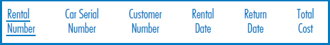
Next, assume that the following table, which has data about the president of each manufacturer, has been added to the database:

Since each company has exactly one president, there is a one-to-one relationship between manufacturers, represented by the existing MANUFACTURER table, and presidents, represented by the new PRESIDENT table. As is usually the case in such situations, it makes sense to represent the two different entities in two different tables. However, if we ever need to retrieve both detailed manufacturer data and detailed president data, we will have to execute a join. If we have to do this frequently and with significant speed, it may make sense to combine the two tables together:

After all, since a company has only one president, it also has only one president name, one president address, and so forth. This arrangement makes for a bulkier table that will be spread out over a larger disk area than either table alone, possibly slowing down certain retrievals. But it will avoid the join needed to retrieve manufacturer and president detailed data together.
Finally, here are examples of the physical design technique of adding new tables. Lucky Rent-A-Car's CAR table is accessed very frequently—so frequently, in fact, that it has become a performance bottleneck. The company has decided to duplicate the table and put each of the two copies on different disk devices so that some applications can access one disk and other applications the other disk. This will improve throughput. However, these two duplicate tables must be kept identical at all times and any changes made to them must be made to both copies simultaneously. Notice that while the CAR table may have to be read frequently for Lucky's rental operations, it has to be updated only when new cars are added to Lucky's inventory or existing cars are taken out of inventory. This makes the duplicate-table technique practical, since frequent changes that require the updating of both tables simultaneously would slow down the entire environment significantly.
In the CUSTOMER table, some large corporate customers' records are accessed much more frequently than the rest of the customer records. To help ease this performance bottleneck and to gather these customer records together in one disk area to further enhance performance, a subset table of copies of just these records can be created and stored elsewhere on the disk or on a different disk. Again, the issue of simultaneous updates of the duplicate data must be considered. Note the difference between creating a subset table and creating a horizontal partition. In the case of subset tables, a copy of the records is left behind in the original table; in the case of horizontal partitioning, no copy is left behind.
SUMMARY
Data is all around us but we normally don't think about it unless we have to use it to keep track of objects that are important to us. The objects and events we come into contact with and their attributes can be noted in structures as simple as lists, which, by extension, we can think of as files and their records.
Moving on to storing data in computers, four basic operations have to be performed: retrieving stored data, inserting new data, deleting stored data, and updating stored data. Applications requiring these operations, in particular the operation of retrieving stored data, may require data to be accessed sequentially while other applications—most of the applications we deal with today—may require data to be accessed on a direct basis.
Disk devices are the predominant secondary memory devices in use today. They are capable of providing both sequential and direct access to data. Disk devices consist of one or more platters on which data can be stored magnetically, mounted on a central spindle. The data is stored on each platter surface in a pattern of concentric circles called tracks. Tracks located one above another on successive surfaces comprise a cylinder.
The arrangement of data on disks is based on a file organization that in turn allows data to be retrieved using an access method. Two such methods for direct access are indexes and hashing. A simple linear index consists of two columns: an ordered list of the identifiers of the records being indexed, each of which is associated in the second column with its physical location on the disk. A more practical arrangement and the one in common use in today's computers is the B+−tree, in which the index is constructed in a hierarchical arrangement. Hashing is a way of arranging the records on the disk based on a mathematical calculation on each record's identifier; retrieval is accomplished using the same mathematical calculation.
Physical database design is the modification of the database structure to improve performance. A variety of factors involving the database structure or its use can adversely affect system performance. In addition to the logical design results, inputs to the physical design process include response time requirements, throughput requirements, and a variety of other data and application characteristics and operational requirements.
Physical database design techniques fall into two categories: techniques that do not change the logical design and techniques that do change the logical design. The former include adding external features such as indexes, reorganizing stored data on the disk, and splitting a table into multiple tables. The latter include adding attributes to a table or changing attributes in a table, combining tables, and adding new tables.
KEY TERMS
B+−tree index
Clustering files
Collision
Cylinder
Data volatility
Data volume
Database performance
Denormalization
Derived data
Disk
Division-remainder method
File organization
Fixed disk drive
Hashing method
Head switching
Horizontal partitioning
Index
Logical view
Overflow records
Performance
Physical database design
Platter
Repeating groups
Response time
Rotational delay
Search attribute
Seek time
Subset tables
Text attribute
Throughput
Track
Transfer time
Vertical partitioning
View
QUESTIONS
- Describe the following disk concepts or components.
- Platter and recording surface.
- Track.
- Cylinder.
- Read/write head.
- Access-arm mechanism.
- Why is it important to store files on a cylinder-by-cylinder basis?
- Describe the four steps in the transfer of data from disk to primary memory.
- What is a file organization? What is an access method? What do they accomplish?
- What is an index? Compare the concept of the index in a book to an index in an information system.
- Describe the idea of the simple linear index. What are its shortcomings?
- What is an indexed-sequential file?
- Describe the idea of the B+−tree index. What are its advantages over the simple linear index?
- Describe how a direct search works using a B+−tree index.
- Describe what happens to the index tree when you insert new records into a file with a B+−tree index.
- Answer the following general questions about indexes:
- Can an index be built over a non-unique field?
- Can an index be built over a field if the file is not stored in sequence by that field?
- Can an index be built over a combination of fields as well as over a single field?
- Is there a limit to the number of indexes that can be built for a file?
- How is an index affected when a change is made to a file? Does every change to a file affect every one of its indexes?
- Can an index be used to achieve sequential access? Explain.
- Describe the idea of the hashed file. What are its advantages and disadvantages in comparison to indexes?
- Describe how a direct search works in a hashed file using the division-remainder method of hashing.
- What is a collision in a hashed file? Why do collisions occur? Why are they of concern in the application environment?
- What is physical database design?
- Describe why physical database design is necessary.
- Explain why the need to perform joins is an important factor affecting application and database performance.
- Why does the degree to which data is dispersed over a disk affect application and database performance?
- Explain why the volume of data access operations can adversely affect application and database performance.
- Which “input” is the starting point for physical database design?
- Describe how response time requirements and throughput requirements determine the overall performance level of the application and database environment.
- Describe the characteristics of the data in the database that must be considered as inputs to the physical database design process. Why are they important?
- Describe the characteristics of the applications that must be considered as inputs to the physical database design process. Why are they important?
- Why do DBMS and hardware characteristics have to be taken into account in the physical design process?
- Explain the statement, “Some physical database design techniques change the logical design and some do not.”
- What attributes should be considered as candidates for having indexes built on them? What is the potential problem with building too many indexes?
- What is a “view”? Which factors affecting application and database performance can be dealt with by using views? Explain.
- Describe the “clustering files” technique. What advantage is gained by using it? What is its disadvantage?
- What is the difference between horizontal and vertical partitioning? What is their common advantage? Are their disadvantages the same or different? Explain.
- Describe the physical design technique of substituting foreign keys. Under what circumstances would you use it?
- Under what circumstances would you want to create a new single-attribute primary key in a table? What would it accomplish?
- Under what circumstances would you want to store derived data in a table? What would it accomplish?
- Combining tables that are in a one-to-one relationship, combining tables involving well controlled repeating groups, and denormalization all lead to the same performance advantage. What is it? Why is it important?
- What is denormalization? Denormalization, while improving performance under certain circumstances, also leads to a serious problem. How does denormalization improve performance and what is this major drawback?
- Duplicating entire tables or parts of tables (“subset tables”) obviously introduces data redundancy. What is the advantage of doing this? Do you think it's worth the introduction of redundancy? Explain.
EXERCISES
- A fixed disk consists of six platters. The upper surface of the topmost platter and the lower surface of the bottommost platter are not used for recording data. There are 120 tracks on each recording surface. How many of each of the following are there in the disk:
- Recording surfaces?
- Cylinders?
- Tracks per cylinder?
- A fixed disk has 80 cylinders. The tracks in each cylinder are numbered 0–11. The upper surface of the topmost platter and the lower surface of the bottommost platter are not used for recording data. How many of each of the following are there in the disk:
- Recording surfaces?
- Platters?
- Tracks per recording surface?
- Consider the B+−tree index, below:
- A record has just been added to Cylinder 6, causing a cylinder split. The highest key value on Cylinder 6 is now 2156, the highest key value on Cylinder 20, and the empty reserve cylinder that received half of Cylinder 6's records is now 2348. Update the tree index accordingly.
- A record has just been added to Cylinder 10, causing a cylinder split. The highest key value on Cylinder 10 is now 3780, the highest key value on Cylinder 25, and the empty reserve cylinder that received half of Cylinder 10's records is now 3900. Update the tree index accordingly. (Note: this question is intended to be independent of the question in part a. Start each of parts a and b from the figure shown.)
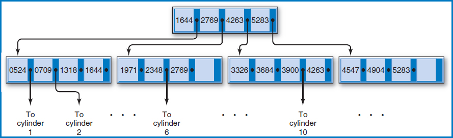
- A hashed file has space for 70 records. Relative record numbers of 0–69 label each of the 70 record positions. In addition, there is space for several overflow (synonym) records. Draw a picture of the file and, using the division-remainder method, store records with each of the following four digit keys, taking collisions into account as necessary:
- 4000.
- 5207.
- 0360.
- 1410.
- Consider the following relational database that Best Airlines uses to keep track of its mechanics, their skills, and their airport locations. Mechanic number, airport name, and skill number are all unique fields. Size is an airport's size in acres. Skill Category is the type of skill, such as an engine skill, wing skill, tire skill, etc. Year Qualified is the year that a mechanic first qualified in a particular skill; Proficiency Rating is the mechanic's proficiency rating in a particular skill.
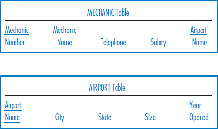

Analyze each of the following situations and, using the physical database design techniques discussed in this chapter, state how you would modify the logical design shown to improve performance or otherwise accommodate it.
- There is a high-priority need to quickly find any particular airport's data given only the airport's city and state.
- There is a frequent need to find the total salary of all of the mechanics at any particular airport.
- There is a high-priority need to quickly find any particular mechanic's data together with the data about the airport at which she works.
- There is a frequent need to list the names and telephone numbers of the mechanics who work at any particular airport, together with the airport's city and state.
- Assume that there is an additional attribute called Skill Description in the SKILL table. This attribute is used to store lengthy descriptions of each skill. The problem is that its presence in the SKILL table is slowing down access to the rest of the data in the table, which is accessed much more frequently.
- The need to access data about the ten largest airports in the country is much more frequent than the need to access data about the rest of the airports.
- Consider the following relational database for the Quality Appliance Manufacturing Co. The database is designed to track the major appliances (refrigerators, washing machines, dishwashers, etc.) that Quality manufactures. It also records information about Quality's suppliers, the parts they supply, the buyers of the finished appliances, and the finished goods inspectors. Note the following facts about this environment:
- Suppliers are the companies that supply Quality with its major components, such as electric motors, for the appliances. Supplier number is a unique identifier.
- Parts are the major components that the suppliers supply to Quality. Each part comes with a part number but that part number is unique only within a supplier. Thus, from Quality's point of view, the unique identifier of a part is the combination of part number and supplier number.
- Each appliance that Quality manufactures is given an appliance number that is unique across all of the types of appliances that Quality makes.
- Buyers are major department stores, home improvement chains, and wholesalers. Buyer numbers are unique.
- An appliance may be inspected by several inspectors. There is clearly a many-to-many relationship between appliances and inspectors.
- There are one-to-many relationships between suppliers and parts (Supplier Number is a foreign key in the PART table), parts and appliances (Appliance Number is a foreign key in the PART table), and appliances and buyers (Buyer Number is a foreign key in the APPLIANCE table).
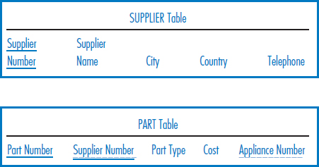
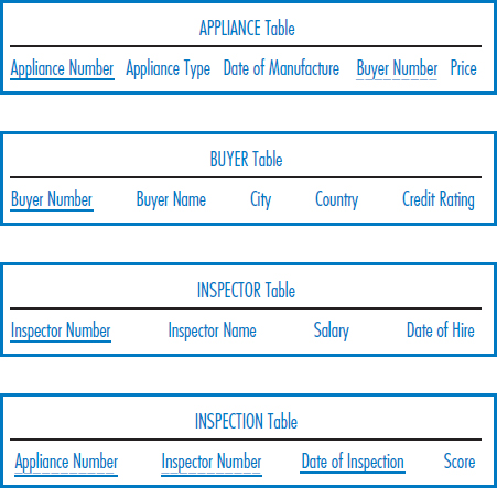
Analyze each of the following situations and, using the physical database design techniques discussed in this chapter, state how you would modify the logical design shown to improve performance or otherwise accommodate it.
- The Appliance Type attribute in the APPLIANCE table indicates whether an appliance is a refrigerator, washing machine, etc. Refrigerator records are accessed much more frequently than those for the other appliance types and there are strict response time requirements for accessing them.
- There is a frequent and very hig- priority need to quickly retrieve detailed data about an appliance together with detailed data about who bought it.
- Because of the large number of people trying to access the PART table and the fast response time needed, the PART table has become a bottleneck and the required response time is not being achieved.
- Assume that the Buyer Name attribute in the BUYER table is unique. There is a high-priority need to quickly retrieve the following data about appliances: appliance number, appliance type, date of manufacture, and buyer name.
- In the APPLIANCE table, there is a much more frequent need with strict response time requirements to access the price data (of course together with the appliance number) than to access the rest of the data in the table.
MINICASES
- Happy Cruise Lines.
Consider the Happy Cruise Lines Sailor file shown below. It lists all the sailors on the company's cruise ships by their unique sailor identification number, their name, the unique identification number of the ship they currently work on, their home country, and their job title.
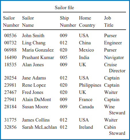
- Create a simple linear index for the Sailor file based on:
- The Sailor Name field.
- The Sailor Number field.
- The Ship Number field.
- The combination of the Ship Number and the Job Title fields.
- Construct a B+−tree index of the type shown in this chapter for the Sailor file, assuming now that there are many more records than are shown above. The file and the index have the following characteristics:
- The file is stored on nine cylinders of the disk. The highest key values on the nine cylinders, in order, are:
- Cylinder 1: 02653
- Cylinder 2: 07784
- Cylinder 3: 13957
- Cylinder 4: 18002
- Cylinder 5: 22529
- Cylinder 6: 27486
- Cylinder 7: 35800
- Cylinder 8: 41633
- Cylinder 9: 48374
- Each index record can hold four key value/pointer pairs.
- There are three index records at the lowest level of the tree index.
- The file is stored on nine cylinders of the disk. The highest key values on the nine cylinders, in order, are:
- The same as part b above, but now there are four index records at the lowest level of the tree index.
- The same as part b above, but each index record can hold two key value/pointer pairs and there are five index records at the lowest level of the tree index.
- Create a simple linear index for the Sailor file based on:
- The Super Baseball League.
Consider the Super Baseball League Player file shown below. It lists all of the players in the league by their unique player identification number, their name, age, the year they joined the league, and the team on which they are currently playing.
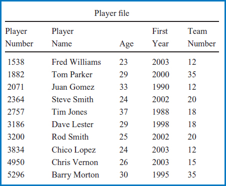
- Create a simple linear index for the Player file based on:
- The Team Number field.
- The Player Name field.
- The Player Number field.
- The combination of the Team Number and the Player Number fields.
- Construct a B+−tree index of the type shown in this chapter for the Player file, assuming that there are now many more records than are shown above. The file and the index have the following characteristics:
- The file is stored on eight cylinders of the disk. The highest key values on the eight cylinders, in order, are:
- Cylinder 1: 1427
- Cylinder 2: 1965
- Cylinder 3: 2848
- Cylinder 4: 3721
- Cylinder 5: 4508
- Cylinder 6: 5396
- Cylinder 7: 6530
- Cylinder 8: 7442
- Each index record can hold four key value/pointer pairs.
- There are three index records at the lowest level of the tree index.
- The file is stored on eight cylinders of the disk. The highest key values on the eight cylinders, in order, are:
- The same as part b above, but now there are four index records at the lowest level of the tree index.
- The same as part b above, but each index record can hold two key value/pointer pairs and there are four index records at the lowest level of the tree index.
- Create a simple linear index for the Player file based on:
- Consider the following relational database for Happy Cruise Lines. It keeps track of ships, cruises, ports, and passengers. A “cruise” is a particular sailing of a ship on a particular date. For example, the seven-day journey of the ship Pride of Tampa that leaves on June 13, 2003, is a cruise. Note the following facts about this environment:
- Both ship number and ship name are unique in the SHIP Table.
- A ship goes on many cruises over time. A cruise is associated with a single ship.
- A port is identified by the combination of port name and country.
- As indicated by the VISIT Table, a cruise includes visits to several ports and a port is typically included in several cruises.
- Both Passenger Number and Social Security Number are unique in the PASSENGER Table. A particular person has a single Passenger Number that is used for all of the cruises that she takes.
- The VOYAGE Table indicates that a person can take many cruises and a cruise, of course, has many passengers.
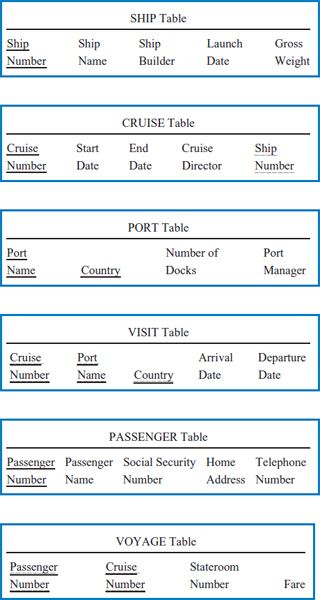
Analyze each of the following situations and, using the physical database design techniques discussed in this chapter, state how you would modify the logical design shown to improve performance or otherwise accommodate it.
- There is a need to list cruises by cruise number but there is also a periodic need to list all of the cruises in order by start date.
- There is a frequent need to quickly retrieve the data about a cruise together with the data about the ship used on the cruise.
- There is a frequent need to quickly retrieve cruise data based on departure date.
- Data about passengers from California must be accessed quickly and much more frequently than data about passengers from anywhere else.
- There is a frequent need to quickly retrieve a list of the port managers of the ports at which the ship on any particular cruise will stop.
- There is a frequent need to quickly find the total number of passengers who were on any particular cruise.
- There is a frequent need to find the start and end dates of cruises as quickly as possible.
- There is a frequent need to find cruise data based on ship name. Hint: The Ship Name attribute is unique.
- Consider the following relational database for the Super Baseball League. It keeps track of teams in the league, coaches and players on the teams, work experience of the coaches, bats belonging to each team, and which players have played on which teams. Note the following facts about this environment:
- The database keeps track of the history of all the teams that each player has played on and all the players who have played on each team.
- The database keeps track of only the current team that a coach works for.
- Team number, team name, and player number are each unique attributes across the league.
- Coach name is unique only within a team (and we assume that a team cannot have two coaches of the same name).
- Serial number (for bats) is unique only within a team.
- In the Affiliation table, the years attribute indicates the number of years that a player played on a team; the batting average is for the years that a player played on a team.
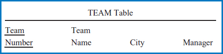
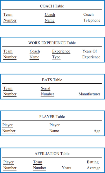
Analyze each of the following situations and, using the physical database design techniques discussed in this chapter, state how you would modify the logical design shown to improve performance or otherwise accommodate it.
- There is a frequent need to quickly find the total number of years that any particular player has played in the league (i.e., the total number of years played for all of the teams a player played for).
- There is a need to retrieve AFFILIATION table records directly based on batting averages.
- The three-attribute primary key of the WORK EXPERIENCE table has been found to be cum-bersome to use in queries and awkward to index.
- There is a frequent very high-priority need to quickly retrieve player name and age data together with the teams (identified by team number) they have played on, the number of years they played on the teams, and the batting averages they compiled.
- Assume that we add the following Stadium table to the Super Baseball League relational database.
Each team has one home stadium, which is what is represented in this table. Assume that a stadium can serve as the home stadium for only one team. Stadium name is unique across the league.
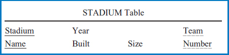
There is a frequent high-priority need to quickly retrieve detailed team and stadium data together.