
CHAPTER 4
RELATIONAL DATA RETRIEVAL: SQL
As we move forward into the discussion of database management systems, we will cover a wide range of topics and skills including how to design databases, how to modify database designs to improve performance, how to organize corporate departments to manage databases, and others. But first, to whet your appetites for what is to come, we're going to dive right into one of the most intriguing aspects of database management: retrieving data from relational databases using the industry-standard SQL database management language.
Note: Some instructors may prefer to cover relational data retrieval with SQL after logical database design, Chapter 7, or after physical database design, Chapter 8. This chapter, Chapter 4 on relational data retrieval with SQL, is designed to work just as well in one of those positions as it is here.
OBJECTIVES
- Write SQL SELECT commands to retrieve relational data using a variety of operators including GROUP BY, ORDER BY, and the built-in functions AVG, SUM, MAX, MIN, COUNT.
- Write SQL SELECT commands that join relational tables.
- Write SQL SELECT subqueries.
- Describe a strategy for writing SQL SELECT statements.
- Describe the principles of a relational query optimizer.
CHAPTER OUTLINE
Introduction
Data Retrieval with the SQL SELECT Command
- Introduction to the SQL SELECT Command
- Basic Functions
- Built-In Functions
- Grouping Rows
- The Join
- Subqueries
- A Strategy for Writing SQL SELECT Commands
Example: Good Reading Book Stores
Example: World Music Association
Example: Lucky Rent-A-Car
Relational Query Optimizer
- Relational DBMS Performance
- Relational Query Optimizer Concepts
Summary
INTRODUCTION
There are two aspects of data management: data definition and data manipulation. Data definition, which is operationalized with a data definition language (DDL), involves instructing the DBMS software on what tables will be in the database, what attributes will be in the tables, which attributes will be indexed, and so forth. Data manipulation refers to the four basic operations that can and must be performed on data stored in any DBMS (or in any other data storage arrangement, for that matter): data retrieval, data update, insertion of new records, and deletion of existing records. Data manipulation requires a special language with which users can communicate data manipulation commands to the DBMS. Indeed, as a class, these are known as data manipulation languages (DMLs).
A standard language for data management in relational databases, known as Structured Query Language or SQL, was developed in the early 1980s. SQL incorporates both DDL and DML features. It was derived from an early IBM research project in relational databases called “System R.” SQL has long since been declared a standard by the American National Standards Institute (ANSI) and by the International Standards Organization (ISO). Indeed, several versions of the standards have been issued over the years. Using the standards, many manufacturers have produced versions of SQL that are all quite similar, at least at the level at which we will look at SQL in this book. These SQL versions are found in such mainstream DBMSs as DB2, Oracle, MS Access, Informix, and others. SQL in its various implementations is used very heavily in practice today by companies and organizations of every description, Advance Auto Parts being one of countless examples.
SQL is a comprehensive database management language. The most interesting aspect of SQL and the aspect that we want to explore in this chapter is its rich data retrieval capability. The other SQL data manipulation features, as well as the SQL data definition features, will be considered in the database design chapters that come later in this book.
DATA RETRIEVAL WITH THE SQL SELECT COMMAND
Introduction to the SQL SELECT Command
Data retrieval in SQL is accomplished with the SELECT command. There are a few fundamental ideas about the SELECT command that you should understand before looking into the details of using it. The first point is that the SQL SELECT command is not the same thing as the relational algebra Select operator discussed in Chapter 5. It's a bit unfortunate that the same word is used to mean two different things, but that's the way it is. The fact is that the SQL SELECT command is capable of performing relational Select, Project, and Join operations singly or in combination, and much more
CONCEPTS IN ACTION
4-A ADVANCE AUTO PARTS
Advance Auto Parts is the second largest retailer of automotive parts and accessories in the U. S. The company was founded in 1932 with three stores in Roanoke, VA, where it is still headquartered today. In the 1980s, with fewer than 175 stores, the company developed an expansion plan that brought it to over 350 stores by the end of 1993. It has rapidly accelerated its expansion since then and, with mergers and acquisitions, now has more than 2,400 stores and over 32,000 employees throughout the United States. Advance Auto Parts sells over 250,000 automotive components. Its innovative “Parts Delivered Quickly” (PDQ) system, which was introduced in 1982, allows its customers access to this inventory within 24 hours.
One of Advance Auto Parts' key database applications, its Electronic Parts Catalog, gives the company an important competitive advantage. Introduced in the early 1990s and continually upgraded since then, this system allows store personnel to look up products they sell based on the customer's vehicle type. The system's records include part descriptions, images, and drawings. Once identified, store personnel pull an item from the store's shelves if it's in stock. If it's not in stock, then using the system they send out a real-time request for the part to the home office to check on the part's warehouse availability. Within minutes the part is picked at a regional warehouse and it's on its way. In addition to its in-store use, the system is used by the company's purchasing and other departments.
The system runs on an IBM mid-range system at company headquarters and is built on the SQL Server DBMS. Parts catalog data, in the form of updates, is downloaded weekly from this system to a small server located in each store. Additional data retrieval at headquarters is accomplished with SQL. The 35-table database includes a Parts table with 2.5 million rows that accounts not only for all of the items in inventory but for different brands of the same item. There is also a Vehicle table with 31,000 records. These two lead to a 45-million-record Parts Application table that describes which parts can be used in which vehicles.

Photo Courtesy of Advance Auto Parts
SQL SELECT commands are considered, for the most part, to be “declarative” rather than “procedural” in nature. This means that you specify what data you are looking for rather than provide a logical sequence of steps that guide the system in how to find the data. Indeed, as we will see later in this chapter, the relational DBMS analyzes the declarative SQL SELECT statement and creates an access path, a plan for what steps to take to respond to the query. The exception to this, and the reason for the qualifier “for the most part” at the beginning of this paragraph, is that a feature of the SELECT command known as “subqueries” permits the user to specify a certain amount of logical control over the data retrieval process.
Another point is that SQL SELECT commands can be run in either a “query” or an “embedded” mode. In the query mode, the user types the command at a workstation and presses the Enter key. The command goes directly to the relational DBMS, which evaluates the query and processes it against the database. The result is then returned to the user at the workstation. Commands entered this way can normally also be stored and retrieved at a later time for repetitive use. In the embedded mode, the SELECT command is embedded within the lines of a higher-level language program and functions as an input or “read” statement for the program. When the program is run and the program logic reaches the SELECT command, the program executes the SELECT. The SELECT command is sent to the DBMS which, as in the query-mode case, processes it against the database and returns the results, this time to the program that issued it. The program can then use and further process the returned data. The only tricky part to this is that traditional higher-level language programs are designed to retrieve one record at a time. The result of a relational retrieval command is itself, a relation. A relation, if it consists of a single row, can resemble a record, but a relation of several rows resembles, if anything, several records. In the embedded mode, the program that issued the SQL SELECT command and receives the resulting relation back, must treat the rows of the relation as a list of records and process them one at a time.
SQL SELECT commands can be issued against either the actual, physical database tables or against a “logical view” of one table or of several joined tables. Good business practice dictates that in the commercial environment, SQL SELECT commands should be issued against such logical views rather than directly against the base tables. As we will see later in this book, this is a simple but effective security precaution.
Finally, the SQL SELECT command has a broad array of features and options and we will only cover some of them at this introductory level. But what is also very important is that our discussion of the SELECT command and the features that we will cover will work in all of the major SQL implementations, such as Oracle, MS Access, SQL Server, DB2, Informix, and so on, possibly with minor syntax variations in some cases.
Basic Functions
The Basic SELECT Format In the simplest SELECT command, we will indicate from which table of the database we want to retrieve data, which rows of that table we are interested in, and which attributes of those rows we want to retrieve. The basic format of such a SELECT statement is:
SELECT<columns>
FROM<table>
WHERE<predicates identifying rows to be included>;
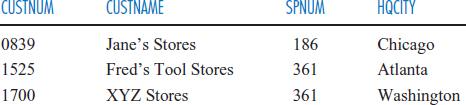
We will illustrate the SQL SELECT command with the General Hardware Co. database of Figure 4.1, which is derived from the General Hardware entity-relationship diagram of Figure 2.9. If you have not as yet covered the database design chapters in this book, just keep in mind that some of the columns are present to tie together related data from different tables, as discussed in Chapter 3. For example, the SPNUM column in the CUSTOMER table is present to tie together related salespersons and customers.
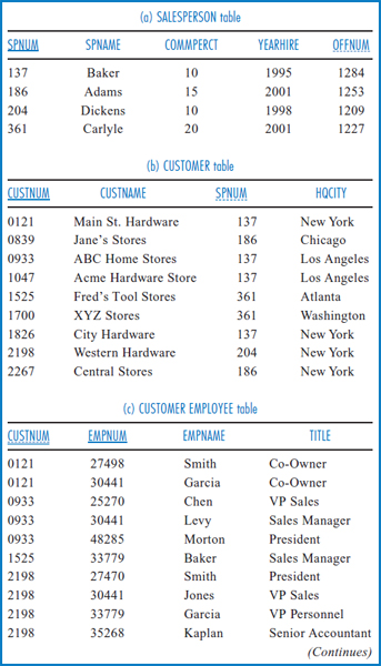
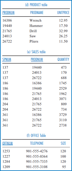
FIGURE 4.1 The General Hardware Company relational database
As is traditional with SQL, the SQL statements will be shown in all capital letters, except for data values taken from the tables. Note that the attribute names in Figure 4.1 have been abbreviated for convenience and set in capital letters to make them easily recognizable in the SQL statements. Also, spaces in the names have been removed. Using the General Hardware database, an example of a simple query that demonstrates the basic SELECT format is:
“Find the commission percentage and year of hire of salesperson number 186.”
The SQL statement to accomplish this would be:
SELECT COMMPERCT, YEARHIRE
FROM SALESPERSON
WHERE SPNUM=186;
How is this command constructed? The desired attributes are listed in the SELECT clause, the required table is listed in the FROM clause, and the restriction or predicate indicating which row(s) is involved is shown in the WHERE clause in the form of an equation. Notice that SELECT statements always end with a single semicolon (;) at the very end of the entire statement.
The result of this statement is:
| COMMPERCT | YEARHIRE |
| 15 | 2001 |
As is evident from this query, an attribute like SPNUM that is used to search for the required rows, also known as a “ search argument,” does not have to appear in the query result, as long as its absence does not make the result ambiguous, confusing, or meaningless.
To retrieve the entire record for salesperson 186, the statement would change to:
SELECT *
FROM SALESPERSON
WHERE SPNUM=186;
resulting in:

The “*” in the SELECT clause indicates that all attributes of the selected row are to be retrieved. Notice that this retrieval of an entire row of the table is, in fact, a relational Select operation (see Chapter 5)! A relational Select operation can retrieve one or more rows of a table, depending, in this simple case, on whether the search argument is a unique or non-unique attribute. The search argument is non-unique in the following query:
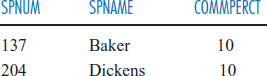
“List the salesperson numbers and salesperson names of those salespersons who have a commission percentage of 10.”
SELECT SPNUM, SPNAME
FROM SALESPERSON
WHERE COMMPERCT=10;
which results in:
| SPNUM | SPNAME |
| 137 | Baker |
| 204 | Dickens |
The SQL SELECT statement can also be used to accomplish a relational Project operation. This is a vertical slice through a table involving all rows and some attributes. Since all of the rows are included in the Project operation, there is no need for a WHERE clause to limit which rows of the table are included. For example,
“List the salesperson number and salesperson name of all of the salespersons.”
SELECT SPNUM, SPNAME
FROM SALESPERSON;
results in:
| SPNUM | SPNAME |
| 137 | Baker |
| 186 | Adams |
| 204 | Dickens |
| 361 | Carlyle |
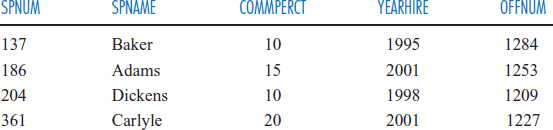
To retrieve an entire table, that is to design an SQL SELECT statement that places no restrictions on either the rows or the attributes, you would issue:
SELECT *
FROM SALESPERSON;
and have as the result:
Comparisons In addition to equal (=), the standard comparison operators, greater than (>), less than (<), greater than or equal to (>=), less than or equal to (<=), and not equal to (<>) can be used in the WHERE clause.
“List the salesperson numbers, salesperson names, and commission percentages of the salespersons whose commission percentage is less than 12.”
SELECT SPNUM, SPNAME, COMMPERCT
FROM SALESPERSON
WHERE COMMPERCT<12;
This results in:
“List the customer numbers and headquarters cities of the customers that have a customer number of at least 1700.”
SELECT CUSTNUM, HQCITY
FROM CUSTOMER
WHERE CUSTNUM>=1700;
results in:
| CUSTNUM | HQCITY |
| 1700 | Washington |
| 1826 | New York |
| 2198 | New York |
| 2267 | New York |
ANDs and ORs Frequently, there is a need to specify more than one limiting condition on a table's rows in a query. Sometimes, for a row to be included in the result it must satisfy more than one condition. This requires the Boolean AND operator. Sometimes a row can be included if it satisfies one of two or more conditions. This requires the Boolean OR operator.
AND An example in which two conditions must be satisfied is:
“List the customer numbers, customer names, and headquarters cities of the customers that are headquartered in New York and that have a customer number higher than 1500.”
SELECT CUSTNUM, CUSTNAME, HQCITY
FROM CUSTOMER
WHERE HQCITY=‘New York’
AND CUSTNUM>1500;
resulting in:
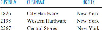
Notice that customer number 0121, which is headquartered in New York, was not included in the results because it failed to satisfy the condition of having a customer number greater than 1500. With the AND operator, it had to satisfy both conditions to be included in the result.
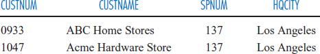
OR To look at the OR operator, let's change the last query to:
“List the customer numbers, customer names, and headquarters cities of the customers that are headquartered in New York or that have a customer number higher than 1500.”
results in:
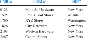
Notice that the OR operator really means one or the other or both. Customer 0121 is included because it is headquartered in New York. Customers 1525 and 1700 are included because they have customer numbers higher than 1500. Customers 1826, 2198, and 2267 are included because they satisfy both conditions.
Both AND and OR What if both AND and OR are specified in the same WHERE clause? AND is said to be “higher in precedence” than OR, and so all ANDs are considered before any ORs are considered. The following query, which has to be worded very carefully, illustrates this point:
“List the customer numbers, customer names, and headquarters cities of the customers that are headquartered in New York or that satisfy the two conditions of having a customer number higher than 1500 and being headquartered in Atlanta.”
SELECT CUSTNUM, CUSTNAME, HQCITY
FROM CUSTOMER
WHERE HQCITY=‘New York’
OR CUSTNUM>1500
AND HQCITY=‘Atlanta’;
The result of this query is:
Notice that since the AND is considered first, one way for a row to qualify for the result is if its customer number is greater than 1500 and its headquarters city is Atlanta. With the AND taken first, it's that combination or the headquarters city has to be New York. Considering the OR operator first would change the whole complexion of the statement. The best way to deal with this, especially if there are several ANDs and ORs in a WHERE clause, is by using parentheses. The rule is that anything in parentheses is done first. If the parentheses are nested, then whatever is in the innermost parentheses is done first and then the system works from there towards the outermost parentheses. Thus, a “safer” way to write the last SQL statement would be:
SELECT CUSTNUM, CUSTNAME, HQCITY
FROM CUSTOMER
WHERE HQCITY=‘New York’
OR (CUSTNUM>1500
AND HQCITY=‘Atlanta’);
If you really wanted the OR to be considered first, you could force it by writing the query as:
SELECT CUSTNUM, CUSTNAME, HQCITY
FROM CUSTOMER
WHERE (HQCITY=‘New York’
OR CUSTNUM>1500)
AND HQCITY=‘Atlanta’;
This would mean that, with the AND outside of the parentheses, both of two conditions have to be met for a row to qualify for the results. One condition is that the headquarters city is New York or the customer number is greater than 1500. The other condition is that the headquarters city is Atlanta. Since for a given row, the headquarters city can't be both Atlanta and New York, the situation looks grim. But, in fact, customer number 1525 qualifies. Its customer number is greater than 1500, which satisfies the OR of the first of the two conditions, and its headquarters city is Atlanta, which satisfies the second condition. Thus, both conditions are met for this and only this row.
BETWEEN, IN, and LIKE BETWEEN, IN, and LIKE are three useful operators. BETWEEN allows you to specify a range of numeric values in a search. IN allows you to specify a list of character strings to be included in a search. LIKE allows you to specify partial character strings in a “wildcard” sense.
BETWEEN Suppose that you want to find the customer records for those customers whose customer numbers are between 1000 and 1700 inclusive (meaning that both 1000 and 1700, as well as all numbers in between them, are included). Using the AND operator, you could specify this as:
SELECT *
FROM CUSTOMER
WHERE (CUSTNUM>=1000
AND CUSTNUM>=1700);
Or, you could use the BETWEEN operator and specify it as:
SELECT *
FROM CUSTOMER
WHERE CUSTNUM BETWEEN 1000 AND 1700;
With either way of specifying it, the result would be:
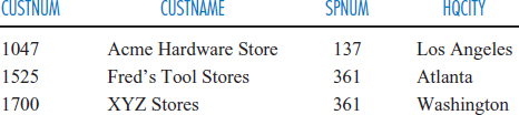
IN Suppose that you want to find the customer records for those customers headquartered in Atlanta, Chicago, or Washington. Using the OR operator, you could specify this as:
SELECT *
FROM CUSTOMER
WHERE (HQCITY=‘Atlanta’
OR HQCITY=‘Chicago’
OR HQCITY=‘Washington’);
Or, you could use the IN operator and specify it as:
SELECT *
FROM CUSTOMER
WHERE HQCITY IN (‘Atlanta’, ‘Chicago’, ‘Washington’);
With either way of specifying it, the result would be:
LIKE Suppose that you want to find the customer records for those customers whose names begin with the letter “A”. You can accomplish this with the LIKE operator and the “%” character used as a wildcard to represent any string of characters. Thus, ‘A%’ means the letter “A” followed by any string of characters, which is the same thing as saying ‘any word that begins with “A”.’
SELECT *
FROM CUSTOMER
WHERE CUSTNAME LIKE ‘A%’;
The result would be:
Note that, unlike BETWEEN and IN, there is no easy alternative way in SQL of accomplishing what LIKE can do.
In a different kind of example, suppose that you want to find the customer records for those customers whose names have the letter “a” as the second letter of their names. Could you specify ‘%a%’? No, because the ‘%a’ portion of it would mean any number of letters followed by “a”, which is not what you want. In order to make sure that there is just one character followed by “a”, which is the same thing as saying that “a” is the second letter, you would specify ‘_a%’. The “_” wildcard character means that there will be exactly one letter (any one letter) followed by the letter “a”. The “%”, as we already know, means that any string of characters can follow afterwards.
SELECT *
FROM CUSTOMER
WHERE CUSTNAME LIKE ‘_a%’;
The result would be:
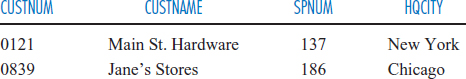
Notice that both the words “Main” and “Jane's” have “a” as their second letter. Also notice that, for example, customer number 2267 was not included in the result. Its name, “Central Stores”, has an “a” in it but it is not the second letter of the name. Again, the single “_” character in the operator LIKE ‘_a%’ specifies that there will be one character followed by “a”. If the operator had been LIKE ‘%a%’, then Central Stores would have been included in the result.
Filtering the Results of an SQL Query Two ways to modify the results of an SQL SELECT command are by the use of DISTINCT and the use of ORDER BY. It is important to remember that these two devices do not affect what data is retrieved from the database but rather how the data is presented to the user.
DISTINCT There are circumstances in which the result of an SQL query may contain duplicate items and this duplication is undesirable. Consider the following query:
“Which cities serve as headquarters cities for General Hardware customers?”
This could be taken as a simple relational Project that takes the HQCITY column of the CUSTOMER table as its result. The SQL command would be:
SELECT HQCITY
FROM CUSTOMER;
which results in:
| HQCITY New York |
| Chicago |
| Los Angeles |
| Los Angeles |
| Atlanta |
| Washington |
| New York |
| New York |
| New York |
Technically, this is the correct result, but why is it necessary to list New York four times or Los Angeles twice? Not only is it unnecessary to list them more than once, but doing so produces unacceptable clutter. Based on the way the query was stated, the result should have each city listed once. The DISTINCT operator is used to eliminate duplicate rows in a query result. Reformulating the SELECT statement as:
SELECT DISTINCT HQCITY
FROM CUSTOMER;
results in:
| HQCITY |
| New York |
| Chicago |
| Los Angeles |
| Atlanta |
| Washington |
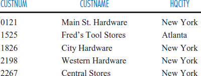
ORDER BY The ORDER BY clause simply takes the results of an SQL query and orders them by one or more specified attributes. Consider the following query:
“Find the customer numbers, customer names, and headquarters cities of those customers with customer numbers greater than 1000. List the results in alphabetic order by headquarters cities.”
SELECT CUSTNUM, CUSTNAME, HQCITY
FROM CUSTOMER
WHERE CUSTNUM>1000
ORDER BY HQCITY;
This results in:
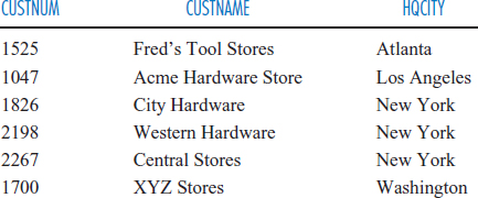
If you wanted to have the customer names within the same city alphabetized, you would write:
SELECT CUSTNUM, CUSTNAME, HQCITY
FROM CUSTOMER
WHERE CUSTNUM>1000
ORDER BY HQCITY, CUSTNAME;
The default order for ORDER BY is ascending. The clause can include the term ASC at the end to make ascending explicit or it can include DESC for descending order.
Built-In Functions
A number of so-called “built-in functions” give the SQL SELECT command additional capabilities. They involve the ability to perform calculations based on attribute values or to count the number of rows that satisfy stated criteria.
AVG and SUM Recall that the SALES table shows the lifetime quantity of particular products sold by particular salespersons. For example, the first row indicates that Salesperson 137 has sold 473 units of Product Number 19440 dating back to when she joined the company or when the product was introduced. Consider the following query:
“Find the average number of units of the different products that Salesperson 137 has sold (i.e., the average of the quantity values in the first three records of the SALES table).”
Using the AVG operator, you would write:
SELECT AVG(QUANTITY)
FROM SALES
WHERE SPNUM=137;
and the result would be:
| AVG(QUANTITY) |
| 443.67 |
To find the total number of units of all products that she has sold, you would use the SUM operator and write:
SELECT SUM(QUANTITY)
FROM SALES
WHERE SPNUM=137;
and the result would be:
| SUM(QUANTITY) |
| 1331 |
MIN and MAX You can also find the minimum or maximum of a set of attribute values. Consider the following query:
“What is the largest number of units of Product Number 21765 that any individual salesperson has sold?”
Using the MAX operator, you would write:
SELECT MAX(QUANTITY)
FROM SALES
WHERE PRODNUM=21765;
and the result would be:
| MAX(QUANTITY) |
| 3110 |
To find the smallest number of units you simply replace MAX with MIN:
SELECT MIN(QUANTITY)
FROM SALES
WHERE PRODNUM=21765;
and get:
| MIN(QUANTITY) |
| 809 |
COUNT COUNT is a very useful operator that counts the number of rows that satisfy a set of criteria. It is often used in the context of “how many of something” meet some stated conditions. Consider the following query:
“How many salespersons have sold Product Number 21765?”
Remember that each row of the SALES table describes the history of a particular salesperson selling a particular product. That is, each combination of SPNUM and PRODNUM is unique; there can only be one row that involves a particular SPNUM/PRODNUM combination. If you can count the number of rows of that table that involve Product Number 21765, then you know how many salespersons have a history of selling it. Using the notational device COUNT(*), the SELECT statement is:
SELECT COUNT(*)
FROM SALES
WHERE PRODNUM=21765;
and the answer is:
| COUNT(*) |
| 3 |
Don't get confused by the difference between SUM and COUNT. As we demonstrated above, SUM adds up a set of attribute values; COUNT counts the number of rows of a table that satisfy a set of stated criteria.
Grouping Rows
Using the built-in functions, we were able to calculate results based on attribute values in several rows of a table. In effect, we formed a single “group” of rows and performed some calculation on their attribute values. There are many situations that require such calculations to be made on several different groups of rows. This is a job for the GROUP BY clause.
GROUP BY A little earlier we found the total number of units of all products that one particular salesperson has sold. It seems reasonable that at some point we might want to find the total number of units of all products that each salesperson has sold. That is, we want to group together the rows of the SALES table that belong to each salesperson and calculate a value—the sum of the Quantity attribute values in this case—for each such group. Here is how such a query might be stated:
“Find the total number of units of all products sold by each salesperson.”
The SQL statement, using the GROUP BY clause, would look like this:
SELECT SPNUM, SUM(QUANTITY)
FROM SALES
GROUP BY SPNUM;
and the results would be:
| SPNUM | SUM(QUANTITY) |
| 137 | 1331 |
| 186 | 9307 |
| 204 | 1543 |
| 361 | 9577 |
Notice that GROUP BY SPNUM specifies that the rows of the table are to be grouped together based on having the same value in their SPNUM attribute. All the rows for Salesperson Number 137 will form one group, all of the rows for Salesperson Number 186 will form another group, and so on. The Quantity attribute values in each group will then be summed—SUM(QUANTITY)—and the results returned to the user. But it is not enough to provide a list of sums:
1331
9307
1543
9577
These are indeed the sums of the quantities for each salesperson But, without identifying which salesperson goes with which sum, they are meaningless! That's why the SELECT clause includes both the SPNUM and the SUM(QUANTITY). Including the attribute(s) specified in the GROUP BY clause in the SELECT clause allows you to properly identify the sums calculated for each group.
An SQL statement with a GROUP BY clause may certainly also include a WHERE clause. Thus, the query:
“Find the total number of units of all products sold by each salesperson whose salesperson number is at least 150.”
would look like:
SELECT SPNUM, SUM(QUANTITY)
FROM SALES
WHERE SPNUM>=150
GROUP BY SPNUM;
and the results would be:
| SPNUM | SUM(QUANTITY) |
| 186 | 9307 |
| 204 | 1543 |
| 361 | 9577 |
HAVING Sometimes there is a need to limit the results of a GROUP BY based on the values calculated for each group with the built-in functions. For example, take the last query above,
“Find the total number of units of all products sold by each salesperson whose salesperson number is at least 150.”
Now modify it with an additional sentence so that it reads:
“Find the total number of units of all products sold by each salesperson whose salesperson number is at least 150. Include only salespersons whose total number of units sold is at least 5000.”
This would be accomplished by adding a HAVING clause to the end of the SELECT statement:
SELECT SPNUM, SUM(QUANTITY)
FROM SALES
WHERE SPNUM>=150
GROUP BY SPNUM
HAVING SUM(QUANTITY)>=5000;
and the results would be:
| SPNUM | SUM(QUANTITY) |
| 186 | 9307 |
| 361 | 9577 |
with Salesperson Number 204, with a total of only 1543 units sold, dropping out of the results.
Notice that in this last SELECT statement, there are two limitations One, that the Salesperson Number must be at least 150, appears in the WHERE clause and the other, that the sum of the number of units sold must be at least 5000, appears in the HAVING clause. It is important to understand why this is so. If the limitation is based on individual attribute values that appear in the database, then the condition goes in the WHERE clause. This is the case with the limitation based on the Salesperson Number value. If the limitation is based on the group calculation performed with the built-in function, then the condition goes in the HAVING clause. This is the case with the limitation based on the sum of the number of product units sold.
The Join
Up to this point, all the SELECT features we have looked at have been shown in the context of retrieving data from a single table. The time has come to look at how the SQL SELECT command can integrate data from two or more tables or “join” them. There are two specifications to make in the SELECT statement to make a join work. One is that the tables to be joined must be listed in the FROM clause. The other is that the join attributes in the tables being joined must be declared and matched to each other in the WHERE clause. And there is one more point. Since two or more tables are involved in a SELECT statement that involves a join, there is the possibility that the same attribute name can appear in more than one of the tables. When this happens, these attribute names must be “qualified” with a table name when used in the SELECT statement. All of this is best illustrated in an example.
Consider the following query, which we discussed earlier in this book:
“Find the name of the salesperson responsible for Customer Number 1525.”
The SELECT statement to satisfy this query is:
SELECT SPNAME
FROM SALESPERSON, CUSTOMER
WHERE SALESPERSON.SPNUM=CUSTOMER.SPNUM
AND CUSTNUM=152;
and the result is:
| SPNAME |
| Carlyle |
Let's take a careful look at this last SELECT statement. Notice that the two tables involved in the join, SALESPERSON and CUSTOMER, are listed in the FROM clause. Also notice that the first line of the WHERE clause:
SALESPERSON.SPNUM = CUSTOMER.SPNUM
links the two join attributes: the SPNUM attribute of the SALESPERSON table (SALESPERSON.SPNUM) and the SPNUM attribute of the CUSTOMER table (CUSTOMER.SPNUM). The notational device of having the table name “.” the attribute name is known as “qualifying” the attribute name. As we said earlier, this qualification is necessary when the same attribute name is used in two or more tables in a SELECT statement. By the way, notice in the SELECT statement that the attributes SPNAME and CUSTNUM don't have to be qualified because each appears in only one of the tables included in the SELECT statement.
Here is an example of a join involving three tables, assuming for the moment that salesperson names are unique:
“List the names of the products of which salesperson Adams has sold more than 2000 units.”
The salesperson name data appears only in the SALESPERSON table and the product name data appears only in the PRODUCT table. The SALES table shows the linkage between the two, including the quantities sold. And so the SELECT statement will be:
SELECT PRODNAME
FROM SALESPERSON, PRODUCT, SALES
WHERE SALESPERSON.SPNUM=SALES.SPNUM
AND SALES.PRODNUM=PRODUCT.PRODNUM
AND SPNAME=‘Adams’
AND QUANTITY>2000;
which results in:
| PRODNAME |
| Hammer |
| Saw |
Subqueries
A variation on the way that the SELECT statement works is when one SELECT statement is “nested” within another in a format known as a subquery. This can go on through several levels of SELECT statements, with each successive SELECT statement contained in a pair of parentheses. The execution rule is that the innermost SELECT statement is executed first and its results are then provided as input to the SELECT statement at the next level up. This procedure can be an alternative to the join. Furthermore, there are certain circumstances in which this procedure must be used. These latter circumstances are common enough and important enough to include in this treatment of the SQL SELECT command.
YOUR TURN
4.1 QUERIES GALORE!
Having a relational database to query in any business environment opens up a new world of information for managers to use to help them run their portion of the business.
QUESTION:
Think about a business environment that you are familiar with from your daily life. It might be a university, a supermarket, a department store, even a sports league. Write a list of ten questions that you would like to be able to ask that would enhance your interaction with that environment. Is it reasonable that a database could be constructed that would support your ability to ask the questions you've come up with? Do you think that you would be able to formulate your questions using SQL? Explain.
Subqueries as Alternatives to Joins Let's reconsider the first join example given above:
“Find the name of the salesperson responsible for Customer Number 1525.”
If you methodically weave through the database tables to solve this, as we discussed earlier in the book, you start at the CUSTOMER table, find the record for Customer Number 1525 and discover in that record that the salesperson responsible for this customer is Salesperson Number 361. You then take that information to the SALESPERSON table where you look up the record for Salesperson Number 361 and discover in it that the salesperson's name is Carlyle. Using a subquery, this logic can be built into an SQL statement as:
SELECT SPNAME
FROM SALESPERSON
WHERE SPNUM=
  (SELECT SPNUM
   FROM CUSTOMER
   WHERE CUSTNUM=1525);
and the result will again be:
| SPNAME |
| Carlyle |
Follow the way that the description given above of methodically solving the problem is reconstructed as a SELECT statement with a subquery. Since the innermost SELECT (the indented one), which constitutes the subquery, is considered first, the CUSTOMER table is queried first, the record for Customer Number 1525 is found and 361 is returned as the SPNUM result. How do we know that only one salesperson number will be found as the result of the query? Because CUSTNUM is a unique attribute, Customer Number 1525 can only appear in one record and that one record only has room for one salesperson number! Moving along, Salesperson Number 361 is then fed to the outer SELECT statement. This, in effect, makes the main query, that is the outer SELECT, look like:
SELECT SPNAME
FROM SALESPERSON
WHERE SPNUM=361;
and this results in:
| SPNAME |
| Carlyle |
Notice, by the way, that in the SELECT statement, there is only one semicolon at the end of the entire statement, including the subquery.
When a Subquery is Required There is a very interesting circumstance in which a subquery is required. This situation is best explained with an example up front. Consider the following query:
“Which salespersons with salesperson numbers greater than 200 have the lowest commission percentage?” (We'll identify salespersons by their salesperson number.)
This seems like a perfectly reasonable request, and yet it turns out to be deceptively difficult. The reason is that the query really has two very different parts. First, the system has to determine what the lowest commission percentage is for salespersons with salesperson numbers greater than 200. Then, it has to see which of these salespersons has that lowest percentage. It's really tempting to try to satisfy this type of query with an SQL SELECT statement like:
SELECT SPNUM, MIN(COMMPERCT)
FROM SALESPERSON
WHERE SPNUM>200;
or, perhaps:
SELECT SPNUM
FROM SALESPERSON
WHERE SPNUM>200
AND COMMPERCT=MIN(COMMPERCT);
But these will not work! It's like asking SQL to perform two separate operations and somehow apply one to the other in the correct sequence. This turns out to be asking too much. But there is a way to do it and it involves subqueries. In fact, what we will do is ask the system to determine the minimum commission percentage first, in a subquery, and then use that information in the main query to determine which salespersons have it:
SELECT SPNUM
FROM SALESPERSON
WHERE SPNUM>200
AND COMMPERCT=
   (SELECT MIN(COMMPERCT)
    FROM SALESPERSON)
    WHERE SPNUM>200);
which results in:
| SPNUM |
| 204 |
The minimum commission percentage across all of the salespersons with salesperson numbers greater than 200 is determined first in the subquery and the result is 10. The main query then, in effect, looks like:
which yields the result of salesperson number 204, as shown.
Actually, this is a very interesting example of a required subquery. What makes it really interesting is why the predicate, SPNUM>200, appears in both the main query and the subquery. Clearly it has to be in the subquery because you must first find the lowest commission percentage among the salespersons with salesperson numbers greater than 200. But then why does it have to be in the main query, too? The answer is that the only thing that the subquery returns to the main query is a single number, specifically a commission percentage. No memory is passed on to the main query of how the subquery arrived at that value. If you remove SPNUM>200 from the main query, so that it now looks like:
SELECT SPNUM
FROM SALESPERSON
WHERE COMMPERCT=
  (SELECT MIN(COMMPERCT)
   FROM SALESPERSON)
   WHERE SPNUM>200);
you would find every salesperson with any salesperson number whose commission percentage is equal to the lowest commission percentage of the salespersons with salesperson numbers greater than 20. (Of course, if for some reason you do want to find all of the salespersons, regardless of salesperson number, who have the same commission percentage as the salesperson who has the lowest commission percentage of the salespersons with salesperson numbers greater than 20, then this last SELECT statement is exactly what you should write!)
A Strategy for Writing SQL SELECT Commands
Before we go on to some more examples, it will be helpful to think about developing a strategy for writing SQL SELECT statements. The following is an ordered list of steps.
- Determine what the result of the query is to be and write the needed attributes and functions in the SELECT clause. This may seem an obvious instruction, but it will really pay to think this through carefully before going on. In fact, it is at this very first step that you must determine whether the query will require a GROUP BY clause or a subquery. If either of these is required, you should start outlining the overall SELECT statement by writing the GROUP BY clause or the nested SELECT for the subquery further down the page (or screen).
- Determine which tables of the database will be needed for the query and write their names in the FROM clause. Include only those tables that are really necessary for the query. Sometime this can be tricky. For example, you might need an attribute that is the primary key of a table and you might be tempted immediately to include that table in the FROM clause. However, it could be that the attribute in question is a foreign key in another table that is already in the FROM clause for other reasons. It is then unnecessary to include the table in which it is the primary key unless, of course, other attributes from that table are needed, too.
- Begin constructing the WHERE clause by equating the join attributes from the tables that are in the FROM clause. Once this job is out of the way, you can begin considering the row limitations that must be stated in the WHERE clause.
- Continue filling in the details of the WHERE clause, the GROUP BY clause, and any subqueries.
One final piece of advice: If you are new to writing SQL SELECT commands but you have a programming background, you may be tempted to avoid setting up joins and try writing subqueries instead. Resist this temptation, for two reasons! One is that joins are an essential part of the relational database concept. Embrace them; don't be afraid of them. The other is that writing multiple levels of nested subqueries can be extremely error prone and difficult to debug.
EXAMPLE: GOOD READING BOOK STORES
The best way to gain confidence in understanding SQL SELECT statements is to write some! And there are some further refinements of the SQL SELECT that we have yet to present. We will use the same three example databases that appeared in previous chapters but, as with the General Hardware database, we will shorten the attribute names. We will state a variety of queries and then give the SELECT statements that will satisfy them, plus commentary as appropriate. You should try to write the SELECT statements yourself before looking at our solutions!
Figure 4.2 is the Good Reading Bookstores relational database. Here is a list of queries for Good Reading Bookstores.
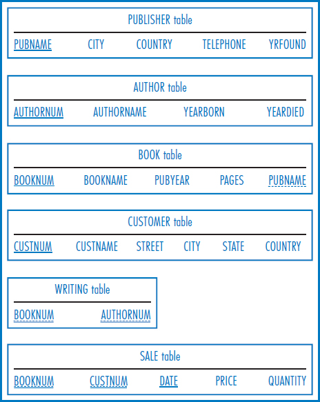
FIGURE 4.2 Good reading Bookstores Relational database
“Find the book number, book name, and number of pages of all the books published by London Publishing Ltd. List the results in order by book name.”
This query obviously requires the PUBNAME attribute but it does not require the PUBLISHER table. All of the information needed is in the BOOK table, including the PUBNAME attribute, which is there as a foreign key. The SELECT statement is:
SELECT BOOKNUM, BOOKNAME, PAGES
FROM BOOK
WHERE PUBNAME=‘London Publishing Ltd.’
ORDER BY BOOKNAME;
“How many books of at least 400 pages does Good Reading Bookstores carry that were published by publishers based in Paris, France?”
This is a straightforward join between the PUBLISHER and BOOK tables that uses the built-in function COUNT. All of the attribute names are unique between the two tables, except for PUBNAME, which must be qualified with a table name every time it is used. Notice that ‘Good Reading Bookstores’ does not appear as a condition in the SELECT statement, although it was mentioned in the query. The entire database is about Good Reading Bookstores and no other! There is no BOOKSTORE CHAIN table in the database and there is no STORENAME or CHAINNAME attribute in any of the tables.
SELECT COUNT(*)
FROM PUBLISHER, BOOK
WHERE PUBLISHER.PUBNAME=BOOK.PUBNAME
AND CITY=‘Paris’
AND COUNTRY=‘France’
AND PAGES>=400;
“List the publishers in Belgium, Brazil, and Singapore that publish books written by authors who were born before 1920.”
Sometimes a relatively simple-sounding query can be fairly involved. This query actually requires four tables of the database! To begin with, we need the PUBLISHER table because that's the only place that a publisher's country is stored. But we also need the AUTHOR table because that's where author birth years are stored. The only way to tie the PUBLISHER table to the AUTHOR table is to connect PUBLISHER to BOOK, then to connect BOOK to WRITING, and finally to connect WRITING to AUTHOR. With simple, one-attribute keys such as those in these tables, the number of joins will be one fewer than the number of tables. The FROM clause below shows four tables and the first three lines of the WHERE clause show the three joins. Also, notice that since a publisher may have published more than one book with the stated specifications, DISTINCT is required to prevent the same publisher name from appearing several, perhaps many, times in the result. Finally, since we want to include publishers in three specific countries, we list the three countries as Belgium, Brazil, and Singapore. But, in the SELECT statement, we have to indicate that for a record to be included in the result, the value of the COUNTRY attribute must be Belgium, Brazil or Singapore.
“How many books did each publisher in Oslo, Norway; Nairobi, Kenya; and Auckland, New Zealand, publish in 2001?”
The keyword here is “each.” This query requires a separate total for each publisher that satisfies the conditions. This is a job for the GROUP BY clause. We want to group together the records for each publisher and count the number of records in each group. Each line of the result must include both a publisher name and count of the number of records that satisfy the conditions. This SELECT statement requires both a join and a GROUP BY. Notice the seeming complexity but really the unambiguous beauty of the ANDs and ORs structure regarding the cities and countries.
SELECT PUBNAME, CITY, COUNTRY, COUNT(*)
FROM PUBLISHER, BOOK
WHERE PUBLISHER.PUBNAME=BOOK.PUBNAME
AND ((CITY=‘Oslo’ AND COUNTRY=‘Norway’)
      OR (CITY=‘Nairobi’ AND COUNTRY=‘Kenya’)
      OR (CITY=‘Auckland’ AND COUNTRY=‘New Zealand’))
AND PUBYEAR=2001
GROUP BY PUBNAME;
“Which publisher published the book that has the earliest publication year among all the books that Good Reading Bookstores carries?”
All that is called for in this query is the name of the publisher, not the name of the book. This is a case that requires a subquery. First the system has to determine the earliest publication year, then it has to see which books have that earliest publication year. Once you know the books, their records in the BOOK table give you the publisher names. Since more than one publisher may have published a book in that earliest year, there could be more than one publisher name in the result. And, since a particular publisher could have published more than one book in that earliest year, DISTINCT is required to avoid having that publisher's name listed more than once.
SELECT DISTINCT PUBNAME
FROM BOOK
WHERE PUBYEAR=
  (SELECT MIN(PUBYEAR)
   FROM BOOK);
EXAMPLE: WORLD MUSIC ASSOCIATION
Figure 4.3 is the World Music Association relational database. Here is a list of queries for the World Music Association.
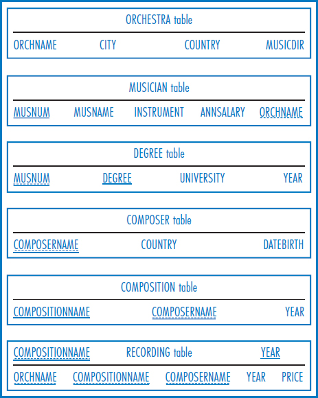
FIGURE 4.3 World Music Association relational database
“What is the total annual salary cost for all the violinists in the Berlin Symphony Orchestra?”
SELECT SUM(ANNSALARY)
FROM MUSICIAN
WHERE ORCHNAME=‘Berlin Symphony Orchestra’
AND INSTRUMENT=‘Violin’;
“Make a single list, in alphabetic order, of all of the universities attended by the cellists in India.”
SELECT DISTINCT UNIVERSITY
FROM ORCHESTRA, MUSICIAN, DEGREE
WHERE ORCHESTRA.ORCHNAME=MUSICIAN.ORCHNAME
AND MUSICIAN.MUSNUM=DEGREE.MUSNUM
AND INSTRUMENT=‘Cello’
AND COUNTRY=‘India’
ORDER BY UNIVERSITY;
“What is the total annual salary cost for all of the violinists of each orchestra in Canada? Include in the result only those orchestras whose total annual salary for its violinists is in excess of $150,000.”
Since this query requires a separate total for each orchestra, the SELECT statement must rely on the GROUP BY clause. Since the condition that the total must be over 150,000 is based on figures calculated by the SUM built-in function, it must be placed in a HAVING clause rather than in the WHERE clause.
SELECT ORCHNAME, SUM(ANNSALARY)
FROM ORCHESTRA, MUSICIAN
WHERE ORCHESTRA.ORCHNAME=MUSICIAN.ORCHNAME
AND COUNTRY=‘Canada’
AND INSTRUMENT=‘Violin’
GROUP BY ORCHNAME
HAVING SUM(ANNSALARY)>150,000;
“What is the name of the most highly paid pianist?”
It should be clear that a subquery is required. First the system has to determine what the top salary of pianists is and then it has to find out which pianists have that salary.
SELECT MUSNAME
FROM MUSICIAN
WHERE INSTRUMENT=‘Piano’
AND ANNSALARY=
  (SELECT MAX(ANNSALARY)
   FROM MUSICIAN
   WHERE INSTRUMENT=‘Piano’);
This is another example in which a predicate, INSTRUMENT=‘Piano’ in this case, appears in both the main query and the subquery. Clearly it has to be in the subquery because you must first find out how much money the highest-paid pianist makes. But then why does it have to be in the main query, too? The answer is that the only thing that the subquery returns to the main query is a single number, specifically a salary value. No memory is passed on to the main query of how the subquery arrived at that value. If you remove INSTRUMENT=‘Piano’ from the main query so that it now looks like:
SELECT MUSNAME
FROM MUSICIAN
WHERE ANNSALARY=
  (SELECT MAX(ANNSALARY)
   FROM MUSICIAN
   WHERE INSTRUMENT=‘Piano’);
you would find every musician who plays any instrument whose salary is equal to the highest-paid pianist. Of course, if for some reason you do want to find all of the musicians, regardless of the instrument they play, who have the same salary as the highest-paid pianist, then this last SELECT statement is exactly what you should write.
“What is the name of the most highly paid pianist in any orchestra in Australia?”
This is the same idea as the last query but involves two tables, both of which must be joined in both the main query and the subquery. The reasoning for this is the same as in the last query. The salary of the most highly paid pianist in Australia must be determined first in the subquery. Then that result must be used in the main query, where it must be compared only to the salaries of Australian pianists.
SELECT MUSNAME
FROM MUSICIAN, ORCHESTRA
WHERE MUSICIAN.ORCHNAME=ORCHESTRA.ORCHNAME
AND INSTRUMENT=‘Piano’
AND COUNTRY=‘Australia’
AND ANNSALARY=
  (SELECT MAX(ANNSALARY)
   FROM MUSICIAN, ORCHESTRA
   WHERE MUSICIAN.ORCHNAME=ORCHESTRA.ORCHNAME
   AND INSTRUMENT=‘Piano’
   AND COUNTRY=‘Australia’);
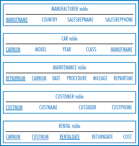
EXAMPLE: LUCKY RENT-A-CAR
Figure 4.4 is the Lucky Rent-A-Car relational database. Here is a list of queries for Lucky Rent-A-Car.
“List the manufacturers whose names begin with the letter “C” or the letter “D” and that are located in Japan.”
SELECT MANUFNAME
FROM MANUFACTURER
FIGURE 4.4 Lucky Rent-A-Car relational database
“What was the average mileage of the cars that had tune-ups in August, 2003?”
SELECT AVG(MILEAGE)
FROM MAINTENANCE
WHERE PROCEDURE=‘Tune-Up’
AND DATE BETWEEN ‘AUG-01-2003’ AND ‘AUG-31-2003’;
The exact format for specifying dates may differ among SQL processors and a given processor may have several options.
“How many different car models are made by manufacturers in Italy?”
This query will use an interesting combination of COUNT and DISTINCT that may not work in all SQL processors. In this case it literally counts the different models among the cars made in Italy. Since many different cars are of the same model, DISTINCT is needed to make sure that each model is counted just once.
SELECT COUNT(DISTINCT MODEL)
FROM MANUFACTURER, CAR
WHERE MANUFACTURER.MANUFNAME=CAR.MANUFNAME
AND COUNTRY=‘Italy’;
“How many repairs were performed on each car manufactured by Superior Motors during the month of March, 2004? Include only cars in the result that had at least three repairs.”
SELECT CAR.CARNUM, COUNT(*)
FROM CAR, MAINTENANCE
WHERE CAR.CARNUM=MAINTENANCE.CARNUM
AND MANUFNAME=‘Superior Motors’
AND DATE BETWEEN ‘MAR-01-2004’ AND ‘MAR-31-2004’
GROUP BY CAR.CARNUM
HAVING COUNT(*)>=3;
“List the cars of any manufacturer that had an oil change in January, 2004, and had at least as many miles as the highest-mileage car manufactured by Superior Motors that had an oil change that same month.”
SELECT MAINTENANCE.CARNUM
FROM MAINTENANCE
WHERE PROCEDURE=‘Oil Change’
AND DATE BETWEEN ‘JAN-01-2004’ AND ‘JAN-31-2004’
AND MILEAGE>=
   (SELECT MAX(MILEAGE)
    FROM CAR, MAINTENANCE
    WHERE CAR.CARNUM, MAINTENANCE.CARNUM
    AND PROCEDURE=‘Oil Change’
    AND DATE BETWEEN ‘JAN-01-2004’ AND ‘JAN-31-2004’
    AND MANUFNAME=‘Superior Motors’);
RELATIONAL QUERY OPTIMIZER
Relational DBMS Performance
An ever-present issue in data retrieval is performance: the speed with which the required data can be retrieved. In a typical relational database application environment, and as we've seen in the examples above, many queries require only one table. It is certainly reasonable to assume that such single-table queries using indexes, hashing, and the like, should, more or less, not take any longer in a relational database system environment than in any other kind of file management system. But, what about the queries that involve joins? Recall the detailed explanation of how data integration works earlier in the book that used the Salesperson and Customer tables as an example. These very small tables did not pose much of a performance issue, even if the join was carried out in the worst-case way, comparing every row of one table to every row of the other table, as was previously described. But what if we attempted to join a 1-million-row table with a 3-million-row table? How long do you think that would take—even on a large, fast computer? It might well take much longer than a person waiting for a response at a workstation would be willing to tolerate. This was actually one of the issues that caused the delay of almost ten years from the time the first article on relational database was published in 1970 until relational DBMSs were first offered commercially almost ten years later.
The performance issue in relational database management has been approached in two different ways. One, the tuning of the database structure, which is known as “physical database design,” will be the subject of an entire chapter of this book, Chapter 8. It's that important. The other way that the relational database performance issue has been approached is through highly specialized software in the relational DBMS itself. This software, known as a relational query optimizer, is in effect an “expert system” that evaluates each SQL SELECT statement sent to the DBMS and determines an efficient way to satisfy it.
Relational Query Optimizer Concepts
All major SQL processors (meaning all major relational DBMSs) include a query optimizer. Using a query optimizer, SQL attempts to figure out the most efficient way of answering a query, before actually responding to it. Clearly, a query that involves only one table should be evaluated to take advantage of aids such as indexes on pertinent attributes. But, again, the most compelling and interesting reason for having a query optimizer in a relational database system is the goal of executing multiple-table data integration or join-type operations without having to go through the worst-case, very time-consuming, exhaustive row-comparison process. Exactly how a specific relational DBMS's query optimizer works is typically a closely held trade secret. Retrieval performance is one way in which the vendors of these products compete with one another. Nevertheless, there are some basic ideas that we can discuss here.
When an SQL query optimizer is presented with a new SELECT statement to evaluate, it seeks out information about the tables named in the FROM clause. This information includes:
- Which attributes of the tables have indexes built over them.
- Which attributes have unique values.
- How many rows each table has.
The query optimizer finds this information in a special internal database known as the “relational catalog,” which will be described further in Chapter 10.
The query optimizer uses the information about the tables, together with the various components of the SELECT statement itself, to look for an efficient way to retrieve the data required by the query. For example, in the General Hardware Co. SELECT statement:
SELECT SPNUM, SPNAME
FROM SALESPERSON
WHERE COMMPERCT=10;
the query optimizer might check on whether the COMMPERCT attribute has an index built over it. If this attribute does have an index, the query optimizer might decide to use the index to find the rows with a commission percentage of 10. However, if the number of rows of the SALESPERSON table is small enough, the query optimizer might decide to read the entire table into main memory and scan it for the rows with a commission percentage of 10.
Another important decision that the query optimizer makes is how to satisfy a join. Consider the following General Hardware Co. example that we looked at above:
SELECT SPNAME
FROM SALESPERSON, CUSTOMER
WHERE SALESPERSON.SPNUM=CUSTOMER.SPNUM
AND CUSTNUM=1525;
In this case, the query optimizer should be able to recognize that since CUSTNUM is a unique attribute in the CUSTOMER table and only one customer number is specified in the SELECT statement, only a single record from the CUSTOMER table, the one for customer number 1525, will be involved in the join. Once it finds this CUSTOMER record (hopefully with an index), it can match the SPNUM value found in it against the SPNUM values in the SALESPERSON records looking for a match. If it is clever enough to recognize that SPNUM is a unique attribute in the SALESPERSON table, then all it has to do is find the single SALESPERSON record (hopefully with an index) that has that salesperson number and pull the salesperson name (SPNAME) out of it to satisfy the query. Thus, in this type of case, an exhaustive join can be completely avoided.
When a more extensive join operation can't be avoided, the query optimizer can choose from one of several join algorithms. The most basic, known as a Cartesian product, is accomplished algorithmically with a “nested-loop join.” One of the two tables is selected for the “outer loop” and the other for the “inner loop.” Each of the records of the outer loop is chosen in succession and, for each, the inner-loop table is scanned for matches on the join attribute. If the query optimizer can determine that only a subset of the rows of the outer or inner tables is needed, then only those rows need be included in the comparisons.
A more efficient join algorithm than the nested-loop join, the “merge-scan join,” can be used only if certain conditions are met. The principle is that for the merge-scan join to work, each of the two join attributes either must be in sorted order or must have an index built over it. An index, by definition, is in sorted order and so, one way or the other, each join attribute has a sense of order to it. If this condition is met, then comparing every record of one table to every record of the other table as in a nested-loop join is unnecessary. The system can simply start at the top of each table or index, as the case may be, and move downwards, without ever having to move upwards.
SUMMARY
SQL has become the standard relational database management data definition and data manipulation language. Data retrieval in SQL is accomplished with the SELECT command. SELECT commands can be run in a direct query mode or embedded in higher-level language programs in an embedded mode. The SELECT command can be used to retrieve one or more rows of a table, one or more columns of a table, or particular columns of particular rows. There are built-in functions that can sum and average data, find the minimum and maximum values of a set of data, and count the number of rows that satisfy a condition. These built-in functions can also be applied to multiple subsets or groups of rows. The SELECT command can also integrate data by joining two or more tables. Subqueries can be developed for certain specific circumstances. There is a strategy for writing SQL commands successfully.
Performance is an important issue in the retrieval of data from relational databases. All relational database management systems have a relational query optimizer, which is software that looks for a good way to solve each relational query presented to it. While the ways that these query optimizers work are considered trade secrets, there are several standard concepts and techniques that they generally incorporate.
KEY TERMS
Access path
AND/OR
Base table
BETWEEN
Built-in functions
Comparisons
Data definition language (DDL)
Data manipulation language (DML)
Declarative
DISTINCT
Embedded mode
Filtering
GROUP BY
HAVING
IN
LIKE
Merge-scan join
ORDER BY
Nested-loop join
Procedural
Query
Relational query optimizer
Search argument
SELECT
Structured Query Language (SQL)
Subquery
QUESTIONS
- What are the four basic operations that can be performed on stored data?
- What is Structured Query Language (SQL)?
- Name several of the fundamental SQL commands and discuss the purpose of each.
- What is the purpose of the SQL SELECT command?
- How does the SQL SELECT command relate to the relational Select, Project, and Join concepts?
- Explain the difference between running SQL in query mode and in embedded mode.
- Describe the basic format of the SQL SELECT command.
- In a general way, describe how to write an SQL SELECT command to accomplish a relational Select operation.
- In a general way, describe how to write an SQL SELECT command to accomplish a relational Project operation.
- In a general way, describe how to write an SQL SELECT command to accomplish a combination of a relational Select operation and a relational Project operation.
- What is the purpose of the WHERE clause in SQL SELECT commands?
- List and describe some of the common operators that can be used in the WHERE clause.
- Describe the purpose of each of the following operators in the WHERE clause:
- AND
- OR
- BETWEEN
- IN
- LIKE
- What is the purpose of the DISTINCT operator?
- What is the purpose of the ORDER BY clause?
- Name the five SQL built-in functions and describe the purpose of each.
- Explain the difference between the SUM and COUNT built-in functions.
- Describe the purpose of the GROUP BY clause. Why must the attribute in the GROUP BY clause also appear in the SELECT clause?
- Describe the purpose of the HAVING clause. How do you decide whether to place a row-limiting predicate in the WHERE clause or in the HAVING clause?
- How do you construct a Join operation in an SQL SELECT statement?
- What is a subquery in an SQL SELECT statement?
- Describe the circumstances in which a subquery must be used.
- What is a relational query optimizer? Why are they important?
- How do relational query optimizers work?
- What information does a relational query optimizer use in making its decisions?
- What are some of the ways that relational query optimizers can handle joins?
EXERCISES
Consider the following relational database that Best Airlines uses to keep track of its mechanics, their skills, and their airport locations. Mechanic number (MECHNUM), airport name (AIRNAME), and skill number are all unique fields. SIZE is an airport's size in acres. SKILLCAT is a skill category, such as an engine skill, wing skill, tire skill, etc. YEARQUAL is the year that a mechanic first qualified in a particular skill; PROFRATE is the mechanic's proficiency rating in a particular skill.
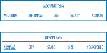
Write SQL SELECT commands to answer the following queries.
- List the names and ages of all the mechanics.
- List the airports in California that are at least 20 acres in size and have been open since 1935. Order the results from smallest to largest airport.
- List the airports in California that are at least 20 acres in size or have been open since 1935.
- Find the average size of the airports in California that have been open since 1935.
- How many airports have been open in California since 1935?
- How many airports have been open in each state since 1935?
- How many airports have been open in each state since 1935? Include in your answer only those states that have at least five such airports.
- List the names of the mechanics who work in California.
- Fan blade replacement is the name of a skill. List the names of the mechanics who have a proficiency rating of 4 in fan blade replacement.
- Fan blade replacement is the name of a skill. List the names of the mechanics who work in California who have a proficiency rating of 4 in fan blade replacement.
- List the total, combined salaries of all of the mechanics who work in each city in California.
- Find the largest of all of the airports.
- Find the largest airport in California.
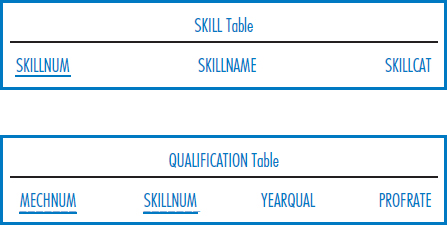
Consider the following relational database for the Quality Appliance Manufacturing Co. The database is designed to track the major appliances (refrigerators, washing machines, dishwashers, etc.) that Quality manufactures. It also records information about Quality's suppliers, the parts they supply, the buyers of the finished appliances, and the finished goods inspectors. Note the following facts about this environment:
- Suppliers are the companies that supply Quality with its major components, such as electric motors, for the appliances. Supplier number is a unique identifier.
- Parts are the major components that the suppliers supply to Quality. Each part comes with a part number but that part number is only unique within a supplier. Thus, from Quality's point of view, the unique identifier of a part is the combination of part number and supplier number.
- Each appliance that Quality manufactures is given an appliance number that is unique across all of the types of appliances that Quality makes.
- Buyers are major department stores, home improvement chains, and wholesalers. Buyer numbers are unique.
- An appliance may be inspected by several inspectors. There is clearly a many-to-many relationship among appliances and inspectors, as indicated by the INSPECTION table.
- There are one-to-many relationships between suppliers and parts (Supplier Number is a foreign key in the PART table), parts and appliances (Appliance Number is a foreign key in the PART table), and appliances and buyers (Buyer Number is a foreign key in the APPLIANCE table).
Write SQL SELECT commands to answer the following queries.
- List the names, in alphabetic order, of the suppliers located in London, Liverpool, and Manchester, UK.
- List the names of the suppliers that supply motors (see PARTTYPE) costing between $50 and $100.
- Find the average cost of the motors (see PARTTYPE) supplied by supplier number 3728.
- List the names of the inspectors who were inspecting refrigerators (see APPLIANCE-TYPE) on April 17, 2011.
- What was the highest inspection score achieved by a refrigerator on November 3, 2011?
- Find the total amount of money spent on Quality Appliance products by each buyer from Mexico, Venezuela, and Argentina.
- Find the total cost of the parts used in each dishwasher manufactured on February 28, 2010. Only include in the results those dishwashers that used at least $200 in parts.
- List the highest0paid inspectors.
- List the highest0paid inspectors who were hired in 2009.
- Among all of the inspectors, list those who earn more than the highest-paid inspector who was hired in 2009.
MINICASES
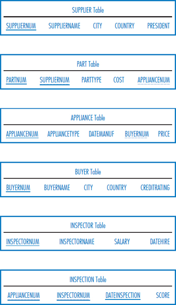
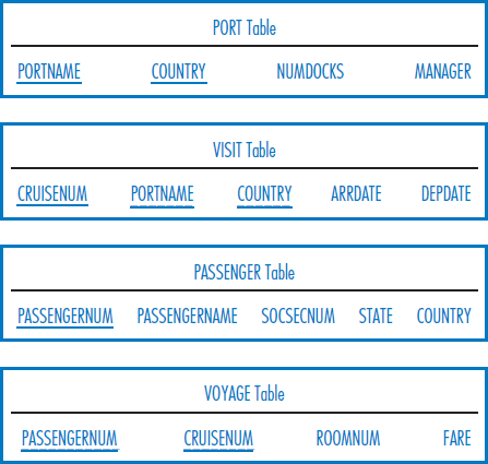
Consider the following relational database for Happy Cruise Lines. It keeps track of ships, cruises, ports, and passengers. A “cruise” is a particular sailing of a ship on a particular date. For example, the seven-day journey of the ship Pride of Tampa that leaves on June 13, 2011, is a cruise. Note the following facts about this environment.
- Both ship number and ship name are unique in the SHIP Table.
- A ship goes on many cruises over time. A cruise is associated with a single ship.
- A port is identified by the combination of port name and country.
- As indicated by the VISIT Table, a cruise includes visits to several ports and a port is typically included in several cruises.
- Both Passenger Number and Social Security Number are unique in the PASSENGER Table. A particular person has a single Passenger Number that is used for all the cruises she takes.
- The VOYAGE Table indicates that a person can take many cruises and a cruise, of course, has many passengers.
Write SQL SELECT commands to answer the following queries.
- Find the start and end dates of cruise number 35218.
- List the names and ship numbers of the ships built by the Ace Shipbuilding Corp. that weigh more than 60,000 tons.
- List the companies that have built ships for Happy Cruise Lines.
- Find the total number of docks in all the ports in Canada.
- Find the average weight of the ships built by the Ace Shipbuilding Corp. that have been launched since 2000.
- How many ports in Venezuela have at least three docks?
- Find the total number of docks in each country. List the results in order from most to least.
- Find the total number of ports in each country.
- Find the total number of docks in each country but include only those countries that have at least twelve docks in your answer.
- Find the name of the ship that operated on (was used on) cruise number 35218.
- List the names, states and countries of the passengers who sailed on The Spirit of Nashville on cruises that began during July, 2011.
- Find the names of the company's heaviest ships.
- Find the names of the company's heaviest ships that began a cruise between July 15, 2011 and July 31, 2011.
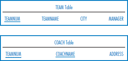
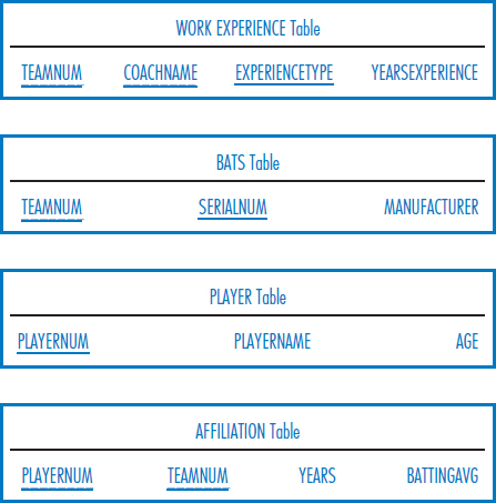
Consider the following relational database for the Super Baseball League. It keeps track of teams in the league, coaches and players on the teams, work experience of the coaches, bats belonging to each team, and which players have played on which teams. Note the following facts about this environment:
- The database keeps track of the history of all the teams that each player has played on and all the players who have played on each team.
- The database only keeps track of the current team that a coach works for.
- Team number, team name, and player number are each unique attributes across the league.
- Coach name is unique only within a team (and we assume that a team cannot have two coaches of the same name).
- Serial number (for bats) is unique only within a team.
- In the Affiliation table, the Years attribute indicates the number of years that a player played on a team; the batting average is for the years that a player played on a team.
Write SQL SELECT commands to answer the following queries.
- Find the names and cities of all of the teams with team numbers greater than 15. List the results alphabetically by team name.
- List all of the coaches whose last names begin with “D” and who have between 5 and 10 years of experience as college coaches (see YEARSEXPERIENCE and EXPERIENCETYPE).
- Find the total number of years of experience of Coach Taylor on team number 23.
- Find the number of different types of experience that Coach Taylor on team number 23 has.
- Find the total number of years of experience of each coach on team number 23.
- How many different manufacturers make bats for the league's teams?
- Assume that team names are unique. Find the names of the players who have played for the Dodgers for at least five years (see YEARS in the AFFILIATION Table.)
- Assume that team names are unique. Find the total number of years of work experience of each coach on the Dodgers, but include in the result only those coaches who have more than eight years of experience.
- Find the names of the league's youngest players.
- Find the names of the league's youngest players whose last names begin with the letter “B”.