Chapter 11
Approaches and Solutions

In previous chapters we have considered a number of challenges to using ad hoc networks, in particular wireless sensor networks. As we discussed earlier, large-scale deployment of wireless sensor networks has become feasible only recently. Until recently, the cost of these nodes was too high, the size of sensor nodes was too large, and the capabilities for sensing and computation were too limited for many applications. Because wireless sensor networks became broadly applicable only a short time ago, the protocols for using sensor nodes and networking them together efficiently are relatively new. Although the protocols will continue to improve and new ideas will be developed, we can recognize a number of general approaches. By reviewing these approaches, the essential ideas that have been developed to date can be understood and evaluated. Future protocols will improve on these protocols, but this progress will benefit from knowledge of the existing protocols.

11.1 Deployment and Configuration

Although configurations vary with the application requirements, general deployments of wireless sensors consist of a large number of inexpensive sensors, each with a limited operating lifetime. Initial placement of the sensors must be done in a cost-effective way, or the advantages of using low-cost sensors are lost in the overhead associated with labor-intensive installation. Periodic replacement of faulty or energy-depleted sensors must be performed to preserve the ability of the sensor networks to meet the application requirements. This too must be accomplished without excessive costs. These considerations have motivated the protocols designed for the initial deployment and configuration, as well as subsequent redeployments to replenish the networks.

11.1.1 Random deployment

To enable limited human interaction in the placement of sensors, random deployment has been suggested. Random deployment occurs because sensors are strewn about the area of interest rather than being placed individually at specific locations. Examples include dropping sensors from an airplane to facilitate military applications that require monitoring enemy troops or a strategically important location (Estrin et al., 1999). In this case, the cost of human-intensive deployment of sensors is not the only consideration; the danger associated with military operations also may prevent manual placement of the sensors. Sensors dropped from the air land in an arbitrary arrangement. The sensor coverage is likely to be less even than manual placement, which may require that extra sensors be used to increase the chance of having sufficient coverage throughout the sensing area. Given the locations of the sensors and the sensing range of each sensor, the coverage of the area of interest can be computed (Meguerdichian et al., 2001). A worst-case analysis could be conducted to figure out how many extra sensors to redeploy.

Another alternative is the use of mobile sensors that can move to better positions after deployment (Zou and Chakrabarty, 2003). The movement can be based on the location of each sensor, the number of sensors in the network, and their ideal positions. This may require on-site coordination among sensor nodes because obstacles or uneven terrain can affect the sensing range and thus their ideal placements.

11.1.2 Scalability

Whether random deployment is employed or some other technique is adopted for positioning the sensors, scalability becomes a concern when many sensors are used. As the number of sensors grows, manual deployment usually grows superlinearly with the size of the network. As the number of nodes increases, additional personnel may be needed to configure the sensors. Furthermore, interaction among neighboring sensors may introduce additional overhead so that increasing the network density leads to a superlinear increase in the deployment overhead.

Because the primary advantages of sensor networks are based on the low cost of the sensors, a large number of sensor nodes will be used to monitor the environment near the point of interest. For this reason, scalability is important in deployment and configuration, as well as the actual sensing functional requirements, such as routing and event detection. To make the configuration process scalable, the process must be at least partially automated. The first step in configuring the network is to organize the nodes into a network. We discuss protocols for this self-organization process in the following section.

11.1.3 Self-organization

For sensor networks of any reasonably large size, some organization into a localized hierarchical structure is useful. Self-organization is the process of nodes in the network imposing some simple scalable organization on the network. Thus self-organization makes the process less labor-intensive, lowering costs and time for deploying the network.

Self-organization can create a number of structures needed for other higher-layer protocols. For example, nodes can self-organize to assign a unique address to each sensor node (Chevallay, Van Dyck, and Hall, 2002), or address size (in bits) can be reduced to reduce the packet overhead (Schurgers, Kulkarni, and Srivastava, 2002). Coordination among sensors is required to ensure that local addresses are unique, which is useful for messages exchanged among neighboring nodes; however, when messages need to be sent to destinations that are farther away, a unique address is required.

Self-organization also has been proposed as a way of creating clusters using the LEACH protocol (Heinzelman, Chandrakasan, and Balakrishnan, 2002). In the simplest case, clusters provide a two-level hierarchy—each sensor forwards readings to the cluster leader (cluster head) responsible for this sensor. The cluster head then aggregates data from multiple sensors and forwards these composite data to the base station.

LEACH proposes a number of different techniques for choosing cluster heads. In the most basic case, cluster heads select themselves using a random number based on the number of sensors in the network, the number of sensors that should serve as cluster heads at any point in time, and how long it has been since this sensor was a cluster head. Based on this information, some randomly chosen nodes become cluster heads. Nodes that do not become cluster heads listen for signals from neighboring cluster heads. A sensor joins the cluster of the cluster head with the strongest received signal. Because cluster heads are chosen randomly, the performance of the network could be poor if the cluster heads do not have a roughly uniform distribution. For example, if all cluster heads end up on one-half of the sensor area, the nodes on the other side of the region will have to expend much more energy to reach a cluster head. Even if the clusters exhibit a better distribution, there is a reasonable possibility that the number of nodes per cluster will not be uniform. For this reason, other options, such as allowing the base station to select the cluster heads or having some other fixed rotation among the sensor nodes may perform better (Heinzelman, 2000).

11.1.4 Security protocol configuration

Security protocols for wireless sensor networks also require configuration (Carman, Kruss, and Matt, 2000). In most cases, security protocols require some authentication and coordination among neighboring sensors. To prevent the compromise of one sensor from compromising the entire sensor network, some pairwise key exchange is required. Unless the positioning of the sensors is predetermined, the identification of neighbors of each sensor node cannot be determined until deployment. Protocols that require preassignment of keys may not work in situations where each pair of neighboring nodes needs a unique key. Because of the potentially large number of sensors being deployed and the limited storage space of each sensor, assigning a key for every potential pair of sensors is not practical. The preassigned keys may be given to sensors that end up not being neighbors. The same problem cannot occur if the sensors are placed manually, but this assumes that no mistakes are made in placing the sensors. If a sensor is misplaced, then these keys cannot be used because communication occurs between neighboring nodes, and the absence of keys between physically neighboring nodes prevents secure communication. Tracking down such erroneous placements could be labor-intensive, leading to substantial delays in the deployment and significantly increasing the cost associated with the sensor deployment. Deployments of additional sensors to replace sensors that are no longer functional also is complicated if these newly deployed sensors must work with some of the sensors that have been deployed already.

Instead, secure communication between neighboring nodes should be established based on some configuration performed after the sensors have been deployed. This requires some key-establishment protocol. To prevent impostors from infiltrating the network, a fixed key that is shared with the base station may be required, although care must be taken to ensure that compromising any sensor node does not result in the entire network being compromised.

Sensor nodes generally communicate with only a subset of the other sensor nodes. For example, communication between a sensor node and the cluster head is needed with a hierarchical organization of the sensor networks. Similarly, each cluster head may need to communicate with a subset of the other cluster heads. Communication with neighboring nodes generally is sufficient for a flat organization. Thus pairwise security keys are needed among only a few of the possible pairs of sensor nodes, but the selection of these pairs cannot be made before deployment of the network unless the nodes are placed carefully, as explained earlier.

The SEKEN protocol (Jamshaid and Schwiebert, 2004) provides a secure protocol for the pairwise key setup in wireless sensor nodes. The protocol assumes that each sensor node is provided with a private device identifier that has been stored in the base station. In addition, the public key of the base station is loaded into each sensor node, which eliminates the need for a trusted certification authority. Each node, starting with the node nearest the base station, forwards a packet to the base station with its device identifier and a timestamp encrypted using the base station’s public key. The base station allocates a key for each sensor node, with sensor nodes that already have been assigned a key forwarding request from another node, e.g., B1, to the base station after appending their own encrypted ID so that the base station can gain some understanding of the network topology. Once more than one node has been assigned a security key, the base station also provides keys that can be shared with the neighboring node that initially forwarded the message for B1. The protocol also handles the addition of more nodes or the removal of nodes. Although the SEKEN protocol supports only a linear array of sensor nodes, extensions to a generic two-dimensional sensor network are possible.

11.1.5 Reconfiguration/redeployment

The lifetime of different sensors within the same network could vary dramatically. The most energy-consuming aspect of sensor operation is communication. Because protocols may place additional demands on some subset of the sensors, such as the sensors near the base station or the sensors far from the base station, redeployment of some sensors may be required to meet the application requirements. Even if most of the sensors are still operational, segments of the sensing field may have inadequate coverage because of the death of sensors in that region.

Redeployment of sensors requires that these newly deployed sensors be incorporated into the existing network. Security keys, locally assigned addresses, and other application-specific parameters that are determined through self-organization need to be supplied to these newly introduced sensors. The existing self-organization network protocols may require a reconfiguration protocol to add new sensor nodes in an already organized network. For example, when using random cluster head selection such as LEACH, it may be necessary to update all the sensors in the network when additional sensors are added. Otherwise, an inadequate or wrong number of cluster heads may be chosen because the number of sensors in the network has changed, and nodes no longer have an accurate estimate of the energy remaining in other nodes.

11.1.6 Location determination

For many sensor applications, the physical location of the sensors is very important. For example, consider an application where the sensors monitor some large area for events, such as a forest fire detection system in a large national park. If an event occurs—a fire starts—the information must be relayed from the sensors that detected the fire to the base station so that the park rangers can be informed. A crucial piece of information is the location of the sensors that detected the fire. Otherwise, the park rangers have no idea where the fire started.

Location information is also useful for routing protocols, where the distance and direction from the source to the destination can be useful for finding routing paths. Location information also can simplify the selection of cluster heads and clusters, as well as other approaches for organizing local groups of sensors. Location information also can be used to perform sleep scheduling or to construct time division multiple access (TDMA) communication schedules. Although knowledge of a node’s neighbors is sufficient for constructing these schedules, position information can make the process more efficient because nodes can compute their own neighbors more easily, as well as their two-hop neighbors, without exchanging several rounds of messages.

Determining the location of individual sensors is not difficult in theory; simply equip each sensor with Global Positioning System (GPS) capabilities, and then each sensor can record and store its location. For stationary sensors, this is particularly attractive because the GPS readings are not required after startup. In practice, however, the cost of equipping each sensor with GPS may make the sensors too expensive. In addition, the added power and size requirements for a GPS receiver also may make these sensors unsuitable for certain applications. Eventually, the cost of GPS receivers will decline, but it will be some time before use of GPS on typical sensors becomes affordable.

One option for addressing this problem is to provide GPS (or manually configured location information) to a subset of the sensor nodes. These sensors then function as beacons or anchors that can be used by other sensors in the network to determine their coordinates (Savvides, Han, and Srivastava, 2001). By listening to several beacons, a node can determine an approximate location. For instance, the distance can be estimated by using the received signal strength (Niculescu and Nath, 2001), by measuring the delay between sonic and radiofrequency (RF) transmissions (Girod et al., 2002; Savvides, Han, and Srivastava, 2001), or simply by considering the transmission range and location of each beacon (Bulusu, Heidemann, and Estrin, 2000; Savarese, Rabaey, and Beutel, 2001). Given the distance between a sensor and at least three beacons, the position of the sensor can be approximated. Once a node has obtained an approximate location, that node can serve as a beacon for other sensors. In Fig. 11.1, for example, node A can be used as a beacon for location information for node B once node A approximates its location. In this way, each sensor obtains an initial estimate of its location using only a few sensors that are equipped with GPS. The initial location estimate is refined further using an iterative approach where each sensor uses additional information from neighboring sensors to obtain a better approximation (Patwari and Hero, 2003; Savarese, Rabaey, and Beutel, 2001). After a series of refinement steps, the sensors achieve a location that has sufficient accuracy for the application. In the forest fire monitoring application, for example, a position that is accurate within, say, 10 m should be satisfactory. Being notified that a fire has started at the sensor location, the smoke and flames should be visible even if the recorded location of the sensor is off by a few meters.

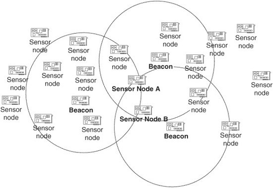
Figure 11.1 Using beacon nodes for location determination.

Another option is to produce a local coordinate system (Bulusu, Heidemann, and Estrin, 2000; Capkun and Hubaux, 2001; Shang et al., 2003). This coordinate system can be used to assign a relative location for each sensor. The coordinate system has its own orientation, although the distances among sensors should be preserved as close to the actual distances as possible. When a sensor detects an event, the relative location within the sensor network needs to be translated into an absolute location that the application can understand. As long as the base station has its absolute physical position, as well as its location based on the relative coordinate system, a translation is possible. Once the base station is incorporated into the local coordinate system, finding a sensor’s location is straightforward. The simplest way to resolve local coordinate systems is to align them. This can be accomplished easily by providing a compass with each sensor node or at least a sufficient number of sensor nodes (Niculescu and Nath, 2003b). With the addition of a compass, the orientation of the device with respect to North can be determined. Using this information to construct the coordinate axes allows the coordinate systems to be aligned. In the absence of a compass to provide a common orientation to the sensor nodes, converging coordinate systems is significantly more difficult.

Another drawback to local coordinate systems is the overhead involved in building and maintaining the coordinates. Especially when nodes are mobile but also as nodes die and more sensors are introduced into the network, updates in the coordinate system may need to propagate throughout the sensor network. Local positioning systems (Capkun and Hubaux, 2001) have been proposed as a technique for defining local coordinate systems without the participation of all the nodes in the network. This idea has been extended to allow the construction of a coordinate system maintained only by the sensors involved in a particular communication (Niculescu and Nath, 2003b). In other words, all nodes on the path from the source to the destination, or on the paths to multiple destinations in the case of group communication, need to share a coordinate system so that messages can be transmitted between the source and the destination(s). Nodes not involved in the communication can be unaware of this coordinate system. This limits the number of nodes that must participate in the construction of the local coordinate system. This may be advantageous when the nodes are mobile because fewer node locations need to be updated, and unneeded information is not maintained. The drawbacks are that a number of local coordinate systems may need to be constructed at any given point in time, there is a time delay associated with building these coordinate systems, and changes in network topology can require that paths be reassembled and additional nodes incorporated into the coordinate system.

The main advantage of using GPS to determine the position of sensors is the flexibility in translating the location into a value that is meaningful to users and network components outside the wireless sensor network. Although having only a few beacon nodes equipped with GPS receivers lowers the cost of deployment, there is still added cost and complexity. In addition, GPS cannot be used inside buildings and other places where GPS signals cannot be received. The main advantage of constructing a local coordinate system is that the limitations, cost, and complexity of using GPS receivers with the sensors are eliminated. The main drawbacks of this approach are that the location determined for each sensor may be less accurate, and constructing the local coordinate system often requires participation of the entire network.

11.2 Routing

Routing is the fundamental component of the network layer protocols. Routing allows the multiple devices that make up the network to exchange information. For this reason, routing in wireless sensor networks has been well studied by the networking research community. A number of protocols have been proposed for routing in wireless sensor networks, and additional protocols continue to be proposed. Each has its own advantages and disadvantages. As with other topics discussed in this chapter, routing in wireless sensor networks is a topic of ongoing research, but many of the core approaches have been identified. Further progress on these different protocols will determine which, if any, of these protocols ends up becoming predominant.

Routing in wireless sensor networks differs from routing in other types of networks for two reasons: (1) the nodes have limited resources for gathering routing information and maintaining routing tables, and (2) the traffic patterns that are generated are likely to be different. The traffic patterns differ because the sensor readings are a primary source of traffic. Some applications accumulate readings peridically, but for many applications, the primary traffic occurs when events are sensed. The sensing and reporting of events are likely to be somewhat random because events are likely to occur in an unpredictable and arbitrary pattern. Once a sensor detects an event, however, tracking that event in the network becomes more predictable. For example, the event may proceed from one location to another along a trajectory that can be predicted with some accuracy (Goel and Imielinski, 2001). Another reason that traffic patterns in wireless sensor networks differ is that the vast majority of the traffic has a base station as either a source or a destination of the message. Communication between two sensors is much less common, with the exception of neighboring sensors that require local collaboration.

When a node senses an event of interest to the application, which is indicated by a sensor reading that is outside the normal operating range, the node must transmit this event to the base station. Of course, some local processing certainly is possible, and this processing may result in some messages being suppressed or combined with the readings of nearby sensors. However, we ignore these considerations in this section. Instead, we focus on the protocols used to transfer sensor readings from the source to the destination once a decision has been made to send this message.

The protocols that we discuss in this section generally assume one of two models. Either all the sensors provide periodic feedback, or the primary source of traffic is from responses from sensors that detect events. The best routing algorithm depends on these traffic characteristics. In some applications, both types of traffic may be required, which warrants using a hybrid approach or using more than one approach.

11.2.1 Event-driven routing

Because sensors interact with the physical world, the data that are routed in the network are based on the readings of the sensors. Rather than having the base station query particular nodes for their current readings, it has been suggested that having the base station query the network for sensor readings with particular characteristics is a more useful model for wireless sensor networks (Intanagonwiwat, Govindan, and Estrin, 2000). For example, the base station might send a request that all nodes that have detected a temperature above 120°F report their readings. This is useful for detecting a fire. The request is flooded throughout the network, and the nodes that respond are those with this reading. In other words, rather than requesting sensor readings from a particular sensor node, we request a particular type of sensor reading from any sensor node that possesses such a reading. This type of network interaction is consistent with the kinds of communications we anticipate from a typical sensor network application.

11.2.2 Periodic sensor readings

Another reasonable type of communication that a sensor network may generate is a periodic response from all the sensors. On a regular basis, all the sensors transmit their sensor readings to the base station (Heinzelman, Chandrakasan, and Balakrishnan, 2002). This gives the base station a snapshot of the entire region covered by the sensors. It also might be useful for diagnosing sensor faults. For example, when a particular sensor has a reading that is not shared by any of the neighboring sensors, it is reasonable to suspect that that sensor is reporting incorrect information because it is either faulty or malicious.

An example application where such periodic readings may need to be accumulated is the temperature monitoring of a large building. If you have ever worked or lived in a large building with multiple floors that has a central heating or air-conditioning system, then you know that the temperature in the building can vary dramatically from room to room. There may be rooms that are uncomfortably cold, whereas other rooms in the same building are unbearably hot. The problem is that the heat distribution is not controlled efficiently so either the heating or air conditioning is not distributed effectively. In some cases, this may result from having too few thermostats or having them placed with a distribution that is less than ideal such as near a computer monitor. An alternative approach to this problem uses a large number of wireless sensors to monitor the temperature in various locations of the building (Kintner-Meyer and Brambley, 2002). For instance, placing sensors in each room, with multiple sensors in a large room, will allow for the accumulation of more data. These data can be used to modify the heating or cooling flow in the building. Not only does this increase the comfort of the building occupants, but also achieves a greater energy efficiency.

It is well known that a system cannot be controlled at a rate faster than the feedback of changes can be obtained. A real-world example is climate control in a car. If the temperature is too hot or too cold, you adjust the output of the heater (or air conditioner). After the adjustment, however, you need to wait until the temperature changes as a result of the change in settings. Otherwise, you simply continue to change things without knowing if you are getting close to your goal—you may simply oscillate between a car that is too hot and too cold. For this reason, some feedback time is required in this system. Sensors measure the temperature and send it to the control center (base station). Based on these measurements, the temperature or distribution of heat is modified. After waiting enough time to ensure that the modifications have affected the system, the sensors take new measurements. Further adjustments then are made. This ongoing cycle can be achieved best by getting periodic readings from all the sensors.

There are two mechanisms for conducting periodic readings. In the first method, each sensor sends its message individually to the base station; in the other method, nodes have a hierarchical structure where nodes transmit their messages to a higher-level node that combines these messages into a single packet that is forwarded higher up the hierarchy. In the case of a two-level hierarchy, for instance, nodes send to their cluster head, which forwards the message directly to the base station. Each of these approaches has advantages and disadvantages, so we consider both approaches. Briefly, sending separate messages to the base station can result in more energy consumption, but combining sensor readings into a single packet can lead to loss of information.

We first consider the idea of sending separate messages. One approach is to send a message directly to the base station from each sensor (Heinzelman, Chandrakasan, and Balakrishnan, 2002). There are two disadvantages to this approach. First, contention for bandwidth becomes acute and severely limits the scalability of this approach. Second, nodes far from the base station expend significantly more energy to transmit their messages. Therefore, the nodes far from the base station deplete their energy much more quickly. On the other hand, if sensors use multihop communication to transmit messages to the base station, then sensors close to the base station must consume a large percentage of their power forwarding messages from other sensors to the base station. This causes the sensors near the base station to run out of energy much sooner than the other nodes in the network.

To avoid either of these situations, nodes can use multihop transmission only when nodes closer to the base station have enough power and memory to perform data forwarding. The base station can send signals to synchronize nodes and create a transmission schedule for the sensor nodes. Even with modest overhead to accumulate the remaining energy levels at the neighbors, the performance of the protocol may better balance energy usage among the sensor nodes. The nodes in the network dissipate their energy at approximately the same rate whether they are close to the base station or far from the base station. This approach is best when the sensor readings cannot be aggregated into a single packet or a few packets. When a high percentage of data aggregation is possible, it is better to aggregate packets at a neighboring node and forward only a single packet or a small number of packets.

When the sensor readings can be aggregated or compressed into a very small fraction of the original data volume, combining or clustering data readings into a single packet and then forwarding only that single packet can save significant amounts of energy. This observation has been incorporated into the LEACH (Heinzelman, Chandrakasan, and Balakrishnan, 2002) and PEGASIS (Lindsey, Raghavendra, and Sivalingam, 2002) protocols.

The simplest version of the LEACH protocol randomly selects a number of the sensor nodes to function as cluster heads, each of which advertises its availability. Each cluster head performs its duties for some period of time, after which different sensors take over the role of cluster head. Since the responsibilities of the cluster head lead to additional energy consumption, periodically changing the cluster heads balances the energy consumption more or less evenly among the sensors throughout the network.

Experiments suggest that having approximately 5 percent of the nodes function as cluster heads at any time gives good performance. Each sensor node that is not a cluster head listens to these advertisements and selects the closest cluster head. Once each cluster head has determined the membership of its cluster, a schedule is created for the transmissions from the sensor nodes in the cluster to the cluster head. On receiving messages from the sensors in this cluster, the cluster head sends a single packet to the base station that combines the readings of all the sensors. The assumption is that each sensor is significantly closer to its cluster head than to the base station. Because the cluster head sends only a single packet a relatively long distance, the amount of energy consumed in communicating with the base station is reduced significantly. This leads to a substantial increase in the lifetime of the sensor nodes.

In LEACH, each sensor chooses the closest cluster head, and the cluster heads are chosen randomly, so there is no assurance as to the distribution of clusters. Since a number of nodes may be assigned to the same cluster, the data may need to be aggregated into a very small fraction of the originally transmitted information. Depending on the application, this level of compression, which is likely to be lossy compression, may or may not be suitable. In some cases, there is a natural trade-off between reducing the power consumption for transmitting information to the base station and obtaining high-quality information at the base station.

Randomly selecting the cluster heads depends on each sensor having some idea of its probability of becoming the cluster head. Each sensor then independently makes a decision on whether or not to become a cluster head. This approach implies that achieving the desired number of cluster heads may not always occur. In some instances, more than an optimal number of sensors may decide to become cluster heads. In other cases, fewer than optimal may. In addition, there is no guarantee that the cluster heads are distributed evenly in a geographic sense. If a poor distribution occurs, some sensors may need to transmit their values a long distance to reach the nearest cluster. In extreme cases, some sensors may send further to reach their chosen cluster head than sending directly to the base station. For these reasons, other options for selecting the cluster heads have been proposed (Heinzelman, 2000). One example is allowing the base station to preselect the cluster heads. This may require sensors to inform the base station periodically of their remaining energy so that sensors can be chosen in a way that extends the life of the entire network as long as possible.

A second approach to aggregating data is the PEGASIS protocol (Lindsey, Raghavendra, and Sivalingam, 2002). In this protocol, a chain of sensors forms starting from sensors far from the base station and ending with the sensors close to the base station. The sensor readings are aggregated on a hop-by-hop basis as they travel through each sensor node. Figure 11.2 shows a possible chain for this sensor network. The messages are aggregated hop by hop until a single packet is delivered to the base station. The chain is created so that each link of the chain is between two nearby sensors to the extent possible. The problem of finding the optimal chain is NP-complete, so the PEGASIS protocol uses a heuristic that produces a reasonably good chain. Since the data are aggregated over short hops, there are no long-distance transmissions from a cluster head to a base station. This reduces the overall energy usage; there are essentially no messages that travel a long distance, provided that there are sensor nodes near the base station. In addition, no cluster heads need to be chosen, which means that the energy requirements placed on each sensor node are roughly equivalent. However, there are two drawbacks to this approach. The first is that a significant delay can occur in transmitting the sensor readings to the base station. Since a sensor must receive the data, process the data, combine these data with the local readings, and then transmit the aggregated data to the next sensor, delay occurs at each sensor in the chain. Since each sensor is included in the chain, the delay grows linearly with the number of sensors in the network.

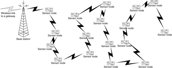
Figure 11.2 Sensor chain for data aggregation.

The delay could become very significant for large sensor networks, and this limits scalability. For many applications, sensor readings must be obtained within some short time after the readings are obtained. When monitoring environmental conditions, timely feedback may be required to react to sensor readings. For instance, the temperature measurements in a high-rise office building may not be delivered for a considerable length of time if they must travel from sensor to sensor throughout every room in the building.

The modified version of the PEGASIS protocol addresses the issue of excessive delay (Lindsey, Raghavendra, and Sivalingam, 2002). In essence, a tree is created so that a hierarchy of nodes is created, and the nodes forward messages up the hierarchy. This results in more energy consumption but reduces the delay from linear time to O (log n) time for n sensors. In fact, the energy-delay product is better with a tree hierarchy because the time decreases much more compared with the increased energy consumption. Any sensor that is not a leaf node in this tree has additional resource demands because it must receive multiple messages and aggregate those messages. However, nodes at higher levels of the hierarchy perform roughly the same amount of work as those at lower layers of the hierarchy, assuming that each parent in the tree has the same number of children. By rotating the responsibility to serve as a parent node, the energy consumption among sensor nodes can be maintained at approximately an equivalent level.

The second drawback is that a very high level of data aggregation is required. Otherwise, the packet size grows significantly. If the sensor readings are all aggregated into a single packet the same size as the original, then either the original packet must be padded to be unnecessarily large, which wastes energy, or the data that eventually reach the base station are a small fraction of the data generated by the sensors. For example, with 100 sensors in the wireless network, the base station receives only about 1 percent of the data produced by the sensors. For some applications, such as counting the number of sensors with a particular reading, this is sufficient. However, for many applications, where the unique reading of each sensor is required, this level of aggregation is not acceptable. On the other hand, if the packet size is permitted to grow, then the energy savings decrease rapidly, and sensors near the base station consume a disproportionately large amount of energy. In fact, unless significant aggregation rates can be obtained, the advantages of hop-by-hop aggregation are limited.

With periodic transmission of the sensor readings from all the sensors in the network, the best choice of protocol depends on the data-aggregation rate. At least some modest data aggregation is always possible because the packet headers from two different messages can be replaced with a single header. Compression or aggregation of the packet data, however, depends on the application requirements and the type of sensor readings obtained. If the application can tolerate some loss of data, then more aggressive compression of the data is possible, which can result in significant energy savings for communication. On the other hand, if only a limited amount of aggregation is possible for a given application, protocols such as LEACH and PEGASIS do not deliver a significant reduction in energy consumption. In extreme cases, where essentially no data aggregation is possible, LEACH and PEGASIS probably consume more energy than protocols that do not rely on data aggregation.

11.2.3 Diffusion routing

As mentioned earlier, routing in wireless sensor networks is either periodic feedback of readings from all the sensors in the network or feedback from sensors that have readings that match particular query values. In the preceding section we considered protocols that support the periodic feedback of readings from the sensors. In this section we consider protocols for routing messages from sensors that have readings that match the requirements of a request from the base station or some other node (Intanagonwiwat, Govindan, and Estrin, 2000).

For purposes of illustration, we assume that the request comes from the base station. Although other network nodes could generate the request, a base station or other gateway node that connects the sensor node with the outside world or a larger network is the most likely source of the queries. The process is initiated by distributing a request from the base station to all the nodes in the network. This generally is accomplished by controlled flooding, except when the request is hard-coded in the sensor application.

Controlled flooding consumes some resources but is the only way to get the request to all the sensor nodes. There are different ways of controlling the flooding. For example, the base station simply could send a message with enough power that it reaches all the sensor nodes. The message also could be sent on a hop-by-hop basis from one sensor node to another. Each sensor would forward a particular request once so that only a limited number of messages are sent. A third option is to forward messages along particular predefined paths or directions so that all the nodes receive the message (Niculescu and Nath, 2003a).

Once the request has been disseminated, the sensors with readings that match the request transmit their readings back to the base station. As an example, we consider an animal-tracking application. Suppose that we are conducting a study of how particular animals move about a certain area. Sensors capable of detecting these animals are deployed in the area of interest. The base station sends a query asking that any sensor that currently detects an animal report the relevant information, such as location and number of animals sensed. The query might include parameters such as the frequency of responses and the length of time the animals should be tracked. The problem then becomes one of routing the information from these sensors back to the base station in an energy-efficient method.

Directed diffusion (Intanagonwiwat, Govindan, and Estrin, 2000) solves this problem by initially sending messages from the sensor nodes to the base station in a reverse flooding operation. Figure 11.3 shows the initial transmission of the query from the base station to the sensor nodes. Messages move toward the base station from each sensor with corresponding readings. Nodes that receive the message and are along a path to the destination forward this message toward the base station. Sensor nodes that receive multiple copies of the same message suppress forwarding. In effect, messages are funneled from individual sensor nodes to the base station.

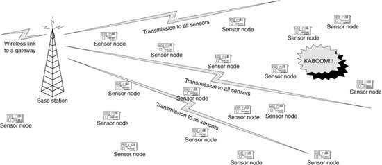
Figure 11.3 Directed diffusion request dissemination.

Figure 11.4 depicts an initial pattern of packet routing from the sensors that detected the event to the base station. Of course, this way of delivering messages to the base station is not particularly energy efficient. To improve the energy efficiency, it is necessary to suppress some of the sensors forwarding messages toward the base station.

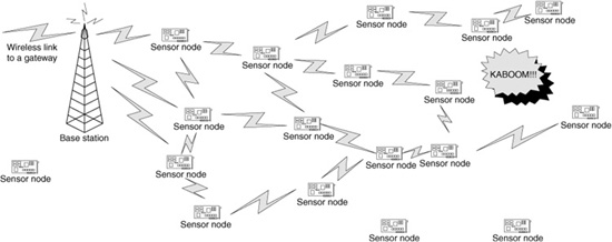
Figure 11.4 Initial processing of an event-driven query.

Figure 11.5 shows one possible set of routing paths that could remain after some duplicate path suppression. The directed diffusion protocol uses both positive and negative feedback to either encourage or discourage sensor nodes from forwarding messages toward the base station. This feedback can be based on, for example, the delay in receiving data. In this case, a sensor that receives the same message from multiple nodes sends positive feedback to the first and negative feedback to the others. Another option is to have a node send with less frequency unless it receives positive reinforcement. In effect, the forwarding of the message times out after some number of packets are forwarded. This is commonly referred to as soft state because the forwarding does not continue unless a message is received periodically to retain this state. This feedback propagates throughout the network to suppress multiple transmissions. Eventually, messages use a single path from the source to the base station.

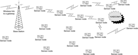
Figure 11.5 Directed diffusion routing paths after redundant path suppression.

Maintaining a single path from each sensor to the base station, perhaps with some data aggregation along this path when similar packets merge from two separate sensors, is the most energy-efficient way of delivering messages to the base station. On the other hand, sensor nodes are less reliable than other network components because the power source is self-contained, and these nodes are relatively inexpensive. For this reason, the probability of delivering a message from a distant sensor to the base station increases if multiple paths are supported. This is especially true when the paths are disjointed or essentially disjointed so that there are no common nodes on these paths.

The trade-off between energy efficiency and the high probability of delivering packets depends on the application’s desired QoS. The best choice of path redundancy also varies based on the characteristics of the sensors, including the mean time to failure and the sleep pattern.

11.2.4 Directional routing

Routing in large sensor networks requires a scalable mechanism for delivering messages. Routing tables are not a good option because sensors have limited storage space, and consuming a large amount of this space for storing routing information is not realistic. Furthermore, centralized routing is not a viable option because contacting a central node in order to determine routing paths is not energy efficient either. Besides, this could add significantly to the routing delay. Although it may be possible to maintain routing paths to a few base stations or other central nodes, general-purpose routing is not scalable if a path for every possible destination needs to be stored and maintained. One method for enabling scalable routing is to have the routing paths implicit in the network. In other words, the routing path is effectively encoded in the network.

For a dense wireless sensor network or mobile ad hoc network, we can assume that, on average, there is sufficient sensor coverage so that a sensor is available in any direction in which we need to route. For example, there could be additional nodes that are approximately North, South, East, and West of the current sensor so that messages can be forwarded in some direction toward the destination. For this type of network, the location of the destination relative to any node in the network is sufficient to determine the orientation in which to route the message. Given the orientation in which the message must be sent, the next sensor that can be used to forward the message can be determined. Figure 11.6 depicts a scenario in which a message is forwarded on a direct line from the sensor node to the base station or as close to a straight line as possible given the positions of the sensor nodes. Each hop of the path is determined on a greedy basis. Although the path in this case follows very closely with the direct path from the sensor to the base station, this is not possible in all cases.

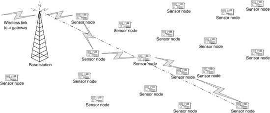
Figure 11.6 Simple example of geographic forwarding.

Various techniques have been proposed for enabling this sort of routing, including Cartesian routing (Finn, 1987), Trajectory-based forwarding (Niculescu and Nath, 2003a), and directional source aware routing (Salhieh et al., 2001). Although each of these protocols differs in their particulars, the general idea is similar—routing messages based on the geographic location of each sensor as well as the destination.

Cartesian routing creates a straight line from the source of the message to the destination. The message is then routed on a hop-by-hop basis through sensors that are on this path. This is particularly useful for mobile nodes because maintaining long routing paths when intermediate nodes are moving on the path is difficult. These nodes may move out of range of the neighboring nodes on the path, thus preventing packets from being forwarded until an alternative path is built when a traditional routing protocol is used. However, no routing path is maintained with Cartesian routing. Instead, when the message arrives at one node, it simply finds the best current node along the path toward the destination and forwards to this node. The node chosen may vary with each packet depending on the mobility patterns and the speed with which nodes move. As long as there is adequate density in the network, there should be a node available at each hop along the path that can forward the message on toward its destination.

With the directional source aware protocol (Salhieh et al., 2001), routing again is done based on the current location and the location of the destination. In order to avoid the need for creating location information for each of the sensors, the sensors are assumed to be distributed in a regular topology. For example, a two-dimensional grid can place the sensor nodes. Although random deployment has some advantages, a regular placement of each sensor leads to a more uniform coverage of the region. In addition, a random deployment of sensors can be augmented with mobile sensors to move these sensors into a more regular distribution. In this case, nodes can perform routing easily as long as each node knows its relative location within the sensor network. Fixed sensors are assumed. Although some initial repositioning of the nodes does not compromise the protocol, support for mobility within the network has not been considered by this protocol. Research on the directional source aware routing protocol (Salhieh and Schwiebert, 2004) has focused on selecting paths for delivering messages between sensor nodes, as well as delivering messages from the sensors to a base station that maintains the lifetime of the sensor network for as long as possible.

Trajectory-based forwarding (Niculescu and Nath, 2003a) is a significant generalization of Cartesian routing. Trajectory-based forwarding uses the geographic location of the ad hoc nodes to determine the route, which avoids having to store routing tables or make use of other centralized routing facilities. Rather than sending along a direct path from the source to the destination, a message can follow any path specified with a parametric equation. For instance, the trajectory could be a sine wave that originates at the source and terminates at the destination (Niculescu and Nath, 2003a). At each hop in the path, nodes forward messages to the most appropriate node toward the destination. The determination of the most appropriate node is made in a number of different ways. For example, the node that is closest to the path of the trajectory, the node that provides the most progress toward the destination while maintaining some close association to the trajectory, or some node that represents a compromise between these two choices could be chosen.

Direction-based routing schemes rely on the position of the current node and the destination in order to deliver messages to the destination. Whether the route is a straight path from the source to the destination or some other path, the intermediate nodes required to deliver the message are not important, so no information is maintained about these nodes. The assumption of sufficient network density guarantees that either there is a suitable candidate node for forwarding the message toward the destination or one will appear shortly because of network mobility. In the absence of mobility, the path may terminate at some point before the destination is reached. An example is when the path is traveling due West, and there is a hole in the network that prevents a message from being forwarded West. In this case, the message must be misrouted—routed temporarily in an incorrect direction—so that the path can be restored later. The best path around a hole cannot be determined using only local information. This requires some additional knowledge of the perimeter of the hole to make the best decision on how to send the message. For example, routing the message North instead of West may result in a very long path, whereas routing the message South instead could lead to a much shorter path. Of course, the opposite situation is also possible, where routing North could be significantly shorter. Without knowledge of the extent of the hole, there is no mechanism for making the correct choice.

A protocol for finding the perimeter of a sensor network, as well as the perimeters of any holes in the network, has been proposed (Martincic and Schwiebert, 2004). The protocol constructs a perimeter at network initialization time by exchanging local information on which nodes are surrounded by neighboring nodes. Nodes that are surrounded by other nodes are not on the edge of the network and are not on the boundary of a hole. By exchanging this local information, the boundaries can be determined without requiring the exchange of global information on the positions of all the sensors. Later the network can make use of the perimeter information for routing, as well as collaboration among neighboring nodes. If there are mobile nodes in the network, then the holes and the boundaries of these holes, as well as the boundary of the entire network, can change. Thus the perimeter information must be updated to maintain valid data for use in routing around obstacles.

11.2.5 Group communication

Routing information from a group of sensors to the base station can be accomplished as individual transmissions from each of these sensors. However, it is more energy efficient to combine these readings into a single message if these sensors are close together and have obtained similar readings. In addition, a higher level of confidence can be placed on the sensor readings if multiple adjacent sensors obtain the same reading. Similarly, a lower level of confidence should be placed on a sensor reading if neighboring sensors that are functioning at the same time do not have the same observation.

In many cases it should be possible to determine that several sensors have generated the same readings using some local communication and local processing. A resource-constrained protocol for combining these sensor readings into a single value with some greater confidence in the correctness of the sensors’ observations should allow this collaboration to be performed on a local basis rather than requiring global communication or the participation of many nodes. Ideally, each node should share information only with other sensors that overlap its sensing range. If the radio transmission range of each sensor is equivalent to at least twice its sensing range, a node can collaborate with all the sensors that overlap any portion of this sensor’s sensing range using direct communication. Figure 11.7 shows the effect of having a radio transmission that is exactly twice the sensing range or slightly less than twice the sensing range. In the first case, sensor node A can communicate with node B. In the second case, the transmission range of node A is less, so although the sensing regions of node A and node B overlap, they cannot communicate with each other directly. The radio transmission range is shown with a solid circle, and the sensing range is shown with a dashed line. This allows each sensor to maintain its own local group of sensors and coordinate readings among these sensors.

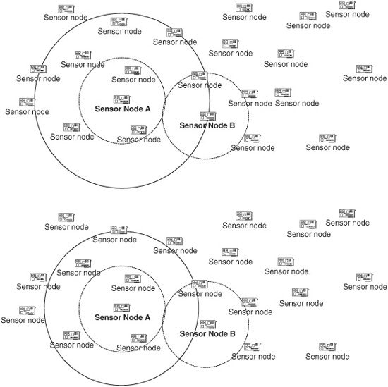
Figure 11.7 Relationship between the sensing range and the transmission range.

A sensor reaches an agreement if a majority of its neighbors have obtained the same reading or one that is approximately the same (Kumar, 2003). If no other neighboring sensors share this same reading, a sensor can assume that there is some problem with its measurement. The measurement then could be retaken, or the sensor could perform other actions to recalibrate the sensor or reset components to try to recover from an error. Malicious sensors could avoid sending an acknowledgment of correct readings to a sensor node but could not prevent a consensus from being reached unless more than half the sensors were malicious or faulty. Sensors also could listen to the request for collaboration and refuse to forward messages from nodes that have not attempted to reach consensus or are transmitting bogus information. These procedures increase the confidence that the base station places in the sensor readings that are obtained from the network. The energy required for transmitting the same reading from the multiple sensors is also reduced significantly. Assuming that each sensor generates a message when it obtains an interesting sensor reading, reducing n sensor readings into a single message saves a significant amount of energy as the value of n increases.

Another option is to combine similar messages as they travel through the network (Intanagonwiwat, Govindan, and Estrin, 2000). As each message approaches the base station, there are fewer remaining paths. Therefore, the probability increases that the message uses a node that has been or will be used for other equivalent messages from other sensors. To combine the messages as they travel through the network, it will be necessary to buffer some packets in order to wait for similar packets to arrive. In addition, some mechanism is required to determine that these packets are synchronized in the sense that the corresponding readings occurred at the same time. We discuss protocols for synchronizing sensor nodes in the next subsection.

Combining messages that record the same event can be done in the network between the sources and the base station whenever the paths used by these sources merge on the way to the base station. These messages can be merged only if they arrive at roughly the same time, or a significant amount of caching delay is introduced between arrival of the first message and arrival of subsequent matching messages. The opportunity to combine matching packets is likely to increase the closer a packet gets to the base station because the number of paths decreases closer to the base station as paths merge. Of course, the advantages of combining packets decreases the closer the packets are to the base station because there are fewer remaining hops. Thus the energy that can be saved by sending a single message instead of multiple messages decreases with fewer hops. The trade-off between the delay in transmitting the packets to the base station and the memory available for caching packets, the difficulty of matching equivalent responses, and the energy consumption for sending multiple messages determines whether this combining is practical. Combining these packets makes sense only when the application can tolerate significant delays and the sensors have sufficient resources for caching these messages. If the application needs to receive the sensor readings as quickly as possible, or if the sensor nodes cannot buffer packets for a substantial period of time, then combining messages within the network is not a realistic option.

11.2.6 Synchronization

Synchronization is an important element of many wireless sensor network applications. As mentioned elsewhere, data aggregation requires synchronization. Collaboration among sensors requires some synchronization. In addition, the base station needs accurate timestamps to perform the data aggregation. TDMA scheduling also requires local synchronization among sensor nodes. Although the synchronization does not always need to be extremely precise, some loose synchronization must be maintained for TDMA scheduling to work correctly.

Keeping all the sensors synchronized with each other would be an expensive operation, especially as the accuracy of the synchronization increases. Since sensors are expected to observe interesting information only occasionally, maintaining close synchronization at all times is not required. Furthermore, a great deal of power could be wasted maintaining synchrony among nodes that do not require it, such as nodes that do not communicate directly with each other. Instead, a protocol has been proposed that keeps a relatively loose level of synchrony among nodes until an event is sensed (Elson and Estrin, 2001). After sensing an event, the sensors establish a more accurate time synchronization, which can be used to determine whether or not events detected by multiple sensors occurred at the same time or not. Based on the locations of these sensors and whether or not the sensors observed an event at the same time, a determination can be made about whether a unique event has been observed by multiple sensors or different events are being reported.

By avoiding the overhead of closely synchronizing the sensors except when an event occurs, the energy requirements are reduced substantially. By synchronizing only when an event is registered, time synchronization is achieved when necessary. Another protocol, such as the Network Time Protocol (Mills, 1994). can be used to maintain loose synchronization among nodes so that closer synchronization can be established when needed. This loose synchronization allows nodes to maintain a schedule that can be used to contact neighboring nodes and establish the close synchronization required when events occur.

Because of the importance of time synchronization for many wireless sensor applications, other efficient synchronization protocols have been proposed. Another synchronization protocol that has been proposed is the Reference Broadcast Synchronization (RBS) protocol (Elson, Girod, and Estrin, 2002). The RBS protocol is a receiver-receiver-based protocol. Although multiple rounds of the RBS protocol can be used to obtain a better estimate, we describe just a single round. The protocol starts with a source sending a signal to two receivers. Each receiver records the time when this signal was received. Based on this, the two receivers determine their relative clock differences, assuming that both nodes take the same amount of time to process the signal after they receive it. There is clock drift among the sensor nodes because no two clocks run at exactly the same rate. Processing multiple signals over a period of time allows the clock drift to be estimated more closely. In addition, the difference in the clocks can be estimated more accurately with multiple samples. In fact, the RBS protocol can achieve synchronization accuracy of several microseconds.

A hierarchical approach can be used for synchronization in wireless sensor networks. This is the approach taken by the Timing-Sync Protocol for Sensor Networks (TPSN) (Ganeriwal, Kumar, and Srivastava, 2003). A root node, which could be a base station, initiates the synchronization process by sending a level_discovery protocol message to each neighbor. These nodes assign their level as level 1 and propagate the message. As the message radiates out from the root node, the levels are assigned based on the minimum number of hops needed to receive this message. Once each node has determined its level in the tree, each pair of nodes that wishes to synchronize sends a message to each other. For example, node A sends a message to node B, which then responds with another message back to node A. By exchanging the timestamps of when these packets were sent and received, the two clocks can be synchronized within a reasonably tight range. This protocol is an example of a sender-receiver synchronization protocol. The TPSN protocol is capable of synchronizing two neighboring nodes within several microseconds.

11.3 Fault Tolerance and Reliability

Ad hoc nodes, and especially mobile nodes, naturally are less reliable than traditional computing devices because communication links are transient. In addition, these nodes are expected to be inexpensive and often do not have the energy resources for long-term operation. For instance, the sensors may be deployed with battery power and replaced after some period of time when the batteries fail. It is unlikely that sensors designed for one-time use will be built with expensive components to prevent failure. It is more likely that the cost of sensor nodes will be modest enough that they can be replaced easily at a lower cost than designing them for long-term use. Sensor nodes also are more susceptible to failure because of their direct exposure to the environment. For these reasons, sensor applications and protocols must be designed with failures and fault recovery as basic assumptions. In other words, not only should the protocols and applications recover from faults, but they also should be designed to operate with the expectation that faults are part of the normal operating situation rather than being anomalous events that should be recovered from so that the application can return to normal operation. Protocols at all layers of the protocol stack must work together to keep faults from preventing the application from receiving correct information or otherwise performing the desired task. In this section we consider a number of protocols at various layers of the traditional protocol stack that could be used to make sensor applications and protocols provide the necessary level of fault tolerance and fault recovery. As can be seen in this discussion, these protocols can operate in conjunction with each other and often perform better together than separately. In other words, the sum is greater than the parts.

11.3.1 FEC and ARQ

Wireless communication is inherently unreliable compared with wired connections. Fiber optic cables, for example, have error rates that are negligible. For all practical purposes, transmission errors on fiber optic cables can be ignored in terms of network performance. Of course, these rare errors must be detected for reliable communications to be supported. However, the protocols can treat such errors as anomalies that should be corrected so that the system can return to the normal operating state as soon as possible. A classic example is the Transmission Control Protocol (TCP), which treats an error as network congestion (a lost packet) rather than a transmission error because errors on wired channels are so rare that handling these special cases separately would not make a significant difference in performance (Jacobson, 1995; Lang and Floreani, 2000). In fact, depending on the mechanism to handle errors, the system performance may decline because the overhead of using this mechanism when almost all packets do not require this mechanism could easily exceed the performance gains when this rare event arises.

Wireless connections, on the other hand, are much less reliable. Bit errors on wireless channels are a normal condition. For this reason, specific techniques are required to operate in the presence of errors. There are two general techniques for addressing bit errors at the physical layer (Lettieri, Schurgers, and Srivastava, 1999). One technique is Forward Error Correction (FEC), which uses extra bits in a packet to allow bit errors to be corrected when they arise during transmission. In general, the more error-correcting bits that are included, the more bit errors that can be corrected. On the other hand, including the number of error-correcting bits in a packet decreases the number of data bits that can be sent or increases the packet size. Automatic Repeat Request (ARQ) refers to a set of protocols used to request retransmission of packets that have errors. There are essentially three choices: (1) stop and wait, which does not send a packet until it receives a positive acknowledgment for the previous packet, (2) go-back-N, which resends all packets from the point at which an error was observed, and (3) selective repeat, which resends only the packets that have errors. Not resending packets that do not have an error saves wireless bandwidth but can require an arbitrarily large buffer. The choice between FEC and ARQ depends on a number of factors, including the error distribution on the wireless channel, whether bursty or uniform error patterns exist, and the probability of bits being erroneous. These two techniques can be used together as a hybrid approach or individually.

11.3.2 Agreement among sensor nodes (Reliability of measurements)

Wireless sensor nodes need to operate under a wide variety of environmental conditions. In addition, wireless sensor nodes are likely to be relatively inexpensive. For these reasons, the sensor readings may have a wide variability in accuracy (Elnahrawy and Nath, 2003). Faulty nodes are discussed in the next section, so in this section we will confine our discussion to sensor readings that are inaccurate because of limitations in the sensing materials. These could be viewed as transient faults, but we consider them to be simply the inherent nature of working with analog sensors; accuracy in a digital sense just is not possible. For this reason, there is an advantage in using redundant sensors—sensors with overlapping areas of sensing—to measure the target phenomenon. These sensors can then collaborate to improve the accuracy of the resulting readings. In other words, by reaching a consensus on interesting readings, sensors can more reliably transfer data to the base station. The other advantage of locally reaching consensus, of course, is that nodes expend less energy in the network in transmitting the sensor readings to the base station.

For wireless sensor networks that have been organized based on hierarchical clustering, there is a straightforward approach to performing consensus because the cluster head simply can combine the information received from each cluster member. The results will then be forwarded up the hierarchy to the base station. The drawback to this approach is that events of interest do not necessarily occur within the boundary of a single cluster. Thus the event may be sensed by nodes in multiple clusters, leading to the transfer of multiple packets, one from each cluster, back to the base station. Depending on the amount of redundancy near the event and how this redundancy is partitioned among adjacent clusters, the clusters may obtain different consensus sensor readings. This could result in the base station receiving multiple readings for the same event and then needing to resolve this discrepancy after receiving these packets. To combat this problem, a recent proposal has been to cluster the wireless sensor network based on the sensing capabilities of the sensors (Kochhal, Schwiebert, and Gupta, 2003). If this is done successfully, the boundaries between adjacent sensors should be better structured to reduce the number of clusters that need to participate in reaching consensus after an event is sensed. The essential idea is to refrain as far as possible from splitting sensors that are very close into separate clusters. Thus events that are near a sensor are likely to be observed primarily by sensors in the same cluster.

When the wireless sensor network is not organized into clusters, there are essentially two options—groups can be formed locally on an ad hoc basis as events occur (Kumar, 2003), or the groups can be formed ahead of time to build consensus when events occur (Gupta and Birman, 2002). An example can best illustrate the difference between these two options. If the groups are preformed, then we have the grouping shown in Fig. 11.8, where the sensors have been partitioned into a grid, and each sensor belongs to the group composed of the sensors in this grid. When an interesting sensor reading is obtained, the other sensors in the same group are consulted, and a consensus is generated with these sensors. The result is then forwarded to the base station.

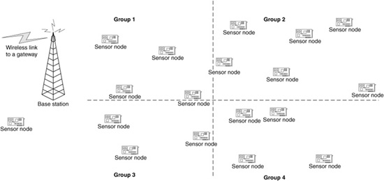
Figure 11.8 A priori grouping of wireless sensors.

Events that occur near a grid edge present challenges for reaching consensus. Either data must be exchanged between adjacent groups, or multiple partial results must be sent toward the base station for further processing. On the other hand, if the group is not formed ahead of time, then when an interesting sensor reading occurs, a node queries its neighbors, those with the same sensing range, for their current readings. Figure 11.9 demonstrates this possibility. An event occurs at some location within the sensor network. A group consisting of the sensors within the circle shown forms with one of these sensors serving as the cluster head. Although the problem of resolving events along grid edges is avoided, some additional delay may be experienced. The nodes then produce consensus by consulting these sensors, and the agreed-on reading is forwarded to the base station.

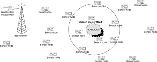
Figure 11.9 Event-triggered grouping of wireless sensors.

The main advantage of forming a group only after an event occurs is that the sensors that are able to observe this event reach consensus among themselves and forward this result to the base station. A second advantage is that the sensors do not need to maintain a great deal of state information. For example, there is no need to maintain a list of sensors within the group because the group forms only after the event occurs. The sensors then reach consensus with the neighbors, but these neighbors can change over time. For example, some sensors may be sleeping or have exhausted their power supplies. Thus a sensor with an interesting reading needs to coordinate only with active neighboring sensors. For wireless sensor networks that have frequent changes in active sensors, maintaining state information on the groups has limited usefulness. The primary disadvantage of this approach is that there is some delay in forming the consensus. Since sensors may not know their neighbors, the group formation must be conducted after an event is observed. Only after the group has been formed on the fly can the consensus-generation process begin. Although there is some added delay in generating consensus, forming the groups after events occur may enable a more accurate consensus value to be generated because all the nodes that could have observed the event are participants in the consensus-forming process.

11.3.3 Dealing with dead or faulty nodes

There are a number of strategies for dealing with dead or faulty nodes. Of course, these nodes cannot be used, but simply ignoring these nodes and operating the network without them may not be acceptable. For example, the dead or faulty nodes may leave holes in the sensor network coverage that prevent the wireless sensor network from performing the desired functions in at least part of the area of interest. Manually repairing or replacing the sensor nodes generally is not an attractive option unless the sensors have a relatively long life span or are costly. When the sensors have been deployed in a remote or inhospitable location, manual replacement may be impossible. Even when it is physically possible to repair or replace the sensors, this may not be a very cost-effective or scalable option.

Rather than replacing or repairing sensors, a better option might be to deploy extra sensors—in effect, creating an initial sensor network that is more dense than necessary. These extra sensors then can sleep until they are needed. For wireless sensors that have renewable energy sources, the sensors could recharge while sleeping. By rotating the active state and sleep state among the wireless sensor nodes, the overall lifetime of the sensor network could be extended in proportion to the additional sensors that are deployed. This has the added advantage of not leaving portions of the sensor network without adequate coverage from the time of failure until the time of repair.

Because faults are somewhat unpredictable, deploying additional sensors uniformly in the wireless sensor network may not be adequate. The failure or depletion of energy may not be uniform. For example, sensors closer to the base station may perform more communication and thus consume energy more rapidly. Even if the additional sensors are not deployed in a nonuniform pattern, such as placing more sensors close to the base station, the problem will not be solved completely. Other instances of sensor failure patterns may be unpredictable when the sensors are deployed. For example, the events concentrated in a particular region of the sensor network may cause these sensors to consume significantly more power than other sensors. Another example would be when most of the sensors in one region are destroyed. As an example, consider an elephant-tracking application. If a herd of elephants happens to stomp through a portion of the sensor network, destroying most of the sensors, the extra sensors that have been deployed will not prevent the sensor coverage from lapsing in this region. An avalanche, mudslide, or flash flood could produce a similar result. An additional localized deployment may be used to recover from such situations, but there is another option.

Mobile sensors could be used to recover from the scenarios such as those just described, where an unanticipated catastrophe occurs in one region of the sensor network (Zou and Chakrabarty, 2003). The extra sensors then could move to the depleted region to fill the hole. Locally coordinating this movement within the sensor network would be quite challenging, so participation of the base station or some other central node in determining when and where to move these extra sensors seems the most practical approach.

11.4 Energy Efficiency

As pointed out repeatedly in the past few chapters, limited energy is one of the primary distinguishing characteristics of wireless sensors. Because wireless communication consumes a relatively large percentage of the power, most of the solutions that have focused on improving energy efficiency have addressed reducing the number of messages generated. However, because wireless sensors have additional components and energy is such a precious commodity, it makes sense to optimize sensor design and operations across all functions.

11.4.1 Uniform power dissipation

One method of ensuring that the sensor network performs its functions as long as possible is to maximize the lifetime of the sensor network. Some authors have defined the network lifetime as the time until the first node dies (Chang and Tassiulas, 2000; Singh, Woo, and Raghavendra, 1998), but this is not a particularly useful metric for wireless sensor networks. Because a large wireless sensor network monitors a relatively large region and there generally is some overlap among the sensors, the death of a single sensor does not significantly reduce the performance of the typical wireless sensor network. In fact, if a single sensor failure did prevent the sensor network from fulfilling its intended task, then the wireless sensor network has no fault tolerance.

Instead, a more reasonable metric is when the sensor network can no longer perform its intended function. Although it is difficult to define this precisely for most applications, designing the protocols so that all the sensors die at roughly the same time or so that sensors die in random locations instead of in specific regions extends the lifetime of the entire sensor network as long as possible. Achieving uniform energy consumption rates is possible for sensor networks that provide periodic feedback to the base station, but for sensor networks that provide only event-driven feedback, organizing the protocols to balance the lifetime of all the sensors is probably impossible.

It is necessary to balance the energy consumption for wireless communication in order to achieve uniform power dissipation. This means that a balance must be found between sending messages on a hop-by-hop basis from the sensor nodes to the base station and sending them directly to the base station. Clustering seems like an attractive solution to this problem, provided that the cluster heads are rotated in a logical manner to balance the energy consumption among the sensors. However, one drawback to clustering is that some of the messages are sent away from the base station in order to reach the cluster head. The information from this sensor then must be sent from the cluster head to the base station, resulting in a larger total distance for the wireless communication. Since the energy used for a wireless communication increases with at least the square of the distance, over time this could become a significant inefficiency in the communication protocol. An approach that achieves a better balance between the two extremes of transmitting directly to the base station and using hop-by-hop communication without the inefficiencies of communicating with the cluster head would be attractive.

In practice, clustering works well when the messages are combined. In other words, when a relatively high percentage of data aggregation is permitted, sending to the cluster head is not likely to reduce the efficiency significantly. Protocols such as LEACH (Heinzelman, Chandrakasan, and Balakrishnan, 2002) and PEGASIS (Lindsey, Raghavendra, and Sivalingam, 2002) are attractive options under these circumstances. On the other hand, the overhead in sending away from the base station in order to reach the cluster head can be costly when little data aggregation is possible. Instead, sending either directly to the base station or forwarding to the neighbor nearest to the base station, depending on the power available, could reduce the overall energy consumption and yield nearly uniform power dissipation. Although some overhead is involved in this approach because the remaining energy must be gathered from the neighbors, the energy consumption of selecting and rotating cluster heads may exceed this overhead. This is especially the case when nodes can gather this information by promiscuous monitoring of transmissions by neighboring nodes.

11.4.2 Sensor component power management

A second option for reducing energy consumption is to decrease the power consumption of a sensor node by powering down various components of a wireless sensor (Sinha and Chandrakasan, 2001). For example, power is consumed by a wireless transceiver whether a sensor is receiving a message or the transceiver is idle, although the power consumption in both cases is less than the energy consumed for transmitting a packet (Chen, Sivalingam, and Agrawal, 1999). However, since wireless sensors send data only sporadically, the power consumption could be very high for leaving the transceiver in an idle state compared with powering down the transceiver (Rabaey et al., 2000). Table 10.1 shows the energy consumed by a few wireless transceivers in each of these three modes.

If a sensor node is sleeping, turning off the wireless transceiver saves a significant fraction of the power. Powering down the sensors and the processor, except for a low-power watchdog process, can extend the lifetime of a wireless sensor for years. However, even when the sensor remains operational, powering down the transceiver can increase the life of the sensor significantly. Many wireless sensor nodes provide a range of power settings that determines which components are powered down and at what level each component is powered down.

Sensor networks should avoid protocols that require turning the transceiver on and off repeatedly over short intervals of time. Because additional energy is consumed in turning the wireless transceiver back on, more energy is consumed than a naive model of the energy consumption would predict (Sinha and Chandrakasan, 2001). Instead, the energy consumption of powering down the transceiver and then powering the transceiver back up should be included in the model. For transceivers that can be powered off for a significant fraction of the time, turning off the transceiver makes sense. However, if the transceiver must be on a significant fraction of the time, or if the intervals between being ready to transmit or receive a packet are short, then turning the sensor off actually might increase the total power consumed.

Some wireless transceivers have a number of power levels, which allow a relatively modest sleeping mode from which the sensor could be returned to full power with less energy. Choosing the best sleep mode for a given sensor is an optimization problem that can be difficult to solve in practice unless the sleeping times can be approximated with a high degree of accuracy and the energy consumption model is accurate. However, an optimal solution may not be necessary. Instead, an approximate solution that yields a significant percentage of the optimal energy savings could be adequate for many applications.

11.4.3 MAC layer protocols

Turning off the wireless transceiver or other sensor components is a physical-layer optimization for saving energy. However, there are other layers of the protocol stack where energy can be saved. For example, energy also can be saved at the MAC layer by scheduling the wireless transmissions. Two sources of overhead can be addressed at the MAC layer. The first is the communication for scheduling the wireless channel. The second is the energy wasted when packet collisions occur and packets must be retransmitted.

Wireless computer communication on typical wireless devices commonly uses the IEEE 802.11 protocol (ANSI, 1999). This protocol optionally sends Request-to-Send (RTS) and Clear-to-Send (CTS) packets to schedule the wireless channel. The other choice is to listen for the availability of the channel prior to transmitting a packet. If the channel is busy, then a node that wishes to send uses an exponential back off to request the wireless channel again at some point in the future. In order to reduce collisions, all nodes need to have their transceivers on so that they can detect the requests from other nodes. This means that even some nodes that are not planning to transmit or receive a message cannot turn off their transceivers or else delay transmission after turning their transceivers back on for some initial listening. In addition, the hidden terminal and exposed terminal problems mean that even with the RTS and CTS scheduling mechanisms, collisions still can occur. For these reasons, IEEE 802.11-type scheduling protocols are not popular for wireless sensor networks. Instead, a different protocol for wireless sensors may be more appropriate.

The most common approach for wireless sensor networks is to use a time division multiple access (TDMA) protocol (Pottie and Kaiser, 2000; Sohrabi et al., 2000). A TDMA protocol divides the wireless channel into different time segments. In each transmission phase, a number of reservation mini-slots are used to reserve each of the transmission slots. Sensors can indicate whether or not they wish to transmit a message during the scheduling time segment. If a sensor is successful in acquiring one of the time slots, then the message can be transmitted during this time interval. One advantage of using a TDMA protocol is that nodes that are not planning to send or receive a packet need to have their transceiver on only during the reservation time slot for the purpose of seeing if other sensors are sending a packet to them. The second advantage is that collisions are avoided, except for relatively small reservation packets, so that the wireless bandwidth can be used efficiently. Eliminating packet retransmissions and allowing inactive sensors to turn off their transceivers for most of the time can save significant power. However, TDMA protocols require that nodes be reasonably well synchronized in order to schedule transmissions during the correct time slot, to ensure that transmissions occur during the correct time slot, and to ensure that the receiver is prepared to receive the message when the transmitter starts the transmission. Since wireless sensor networks usually use hop-by-hop communication or need to schedule communication among only a relatively small set of cluster heads, synchronization on a local basis could be sufficient for achieving the necessary level of time synchrony among the senders and receivers.

11.4.4 Trade-offs between performance and energy efficiency

Energy efficiency also can be obtained at higher layers of the protocol stack, but this usually requires that the application accept more delay. One example is synchronizing the wireless sensors. Maintaining synchronous clocks is very useful when attempting to consolidate readings from multiple sensors—otherwise, it is difficult to determine whether two sensors observed the same event or two distinct events that occurred within a short period of time. However, keeping the sensors synchronized is not possible without a large number of messages and the resulting communication overhead. Instead, the sensors could maintain only loose synchronization and generate tight clock synchronization only after an interesting event occurs (Elson and Estrin, 2001). Although this is a feasible solution in many cases, some added delay is encountered. This additional delay could result in a performance penalty for some real-time applications but also offers significant energy savings.

Another approach to realizing energy savings in a wireless sensor network is to first aggregate data in the wireless sensor network and then to send only the aggregated sensor readings to the base station. This can result in significant energy savings for large sensor networks when the size of the aggregated sensor readings is comparable with the size of a single packet. However, aggregating packets can lead to the loss of information, which can have a negative impact on the performance of the sensor application. In addition, waiting for multiple packets to arrive so that they can be aggregated introduces delay into the transmission process. This delay can produce significant energy savings but does involve a reduction in the application performance for real-time sensor applications.

In essence, any energy-efficiency protocol, whether energy-efficient routing or application-layer protocols, involves some increased delay, loss of accuracy, or other performance penalty. Balancing the energy savings against the performance penalties and achieving the application requirements are one of the challenges in designing wireless sensor networking protocols.

11.5 Summary

In Chap. 11, we have reviewed many wireless sensor networking protocols that have been proposed in the past few years. From this review, we see the novel approaches the researchers have taken to meeting both the requirements and demands of a wireless sensor network. The protocols for using sensor nodes and networking them efficiently are relatively new. Although protocols for these problems will continue to improve and new ideas will be developed, we have seen many general approaches. Future research will improve on these protocols, but this progress will benefit from knowledge of the existing protocols. Therefore, the protocols presented in Chap. 11 are an attractive base upon which to build further research in wireless sensor networking.

11.6 References

ANSI/IEEE Standard 802.11, Wireless LAN Medium Access Control (MAC) Sublayer and ISO/IEC Standard 8802-11, Physical Layer Specifications. 1999.

Bulusu, N., J. Heidemann, and D. Estrin, “GPS-Less Low-Cost Outdoor Localization for Very Small Devices,” IEEE Personal Communications 7(5):28, 2000.

Capkun, M., and J. Hubaux, “GPS-Free Positioning in Mobile Ad-Hoc Networks,” in Proceedings of the 34th Annual Hawaii International Conference on System Science; Island of Maui, IEEE Computer Society, 2001, p. 3481.

Carman, D. W., P. S. Kruss, and B. J. Matt, “Constraints and Approaches for Distributed Sensor Network Security,” in NAI Labs Technical Report 00-010, 2000.

Chang, J., and L. Tassiulas, “Energy Conserving Routing in Wireless Ad-Hoc Networks,” in Annual Joint Conference of the IEEE Computer and Communications Societies (INFOCOM), Vol. 1; Tel-Aviv, Israel, IEEE Computer Society, 2000, p. 22

Chen, J.-C., K. Sivalingam, and P. Agrawal, “Performance Comparison of Battery Power Consumption in Wireless Multiple Access Protocols,” Wireless Networks 5(6):445, 1999.

Chevallay, C., R. E. Van Dyck, and T. A. Hall, “Self-Organization Protocols for Wireless Sensor Networks,” in 36th Annual Conference on Information Sciences and Systems; Princeton, NJ, Princeton University Press, 2002. (Published in CD)

Elnahrawy, E., and B. Nath, “Cleaning and Querying Noisy Sensors,” in ACM International Workshop on Wireless Sensor Networks and Applications; San Diego, CA, ACM, 2003, p. 78.

Elson, J., and D. Estrin, “Time Synchronization for Wireless Sensor Networks,” in International Parallel and Distributed Processing Systems (IPDPS) Workshop on Parallel and Distributed Computing Issues in Wireless Networks and Mobile Computing; San Francisco, CA, IEEE Computer Society, 2001, p. 1965.

Elson, J., L. Girod, and D. Estrin, “Fine-Grained Time Synchronization Using Reference Broadcasts,” in Proceedings of the Fifth Symposium on Operating Systems Design and Implementation (OSDI); Boston, MA, Usenix Association, 2002, p. 147.

Estrin, D., R. Govindan, J. Heidemann, and S. Kumar, “Next Generation Challenges: Scalable Coordination in Sensor Networks,” in International Conference on Mobile Computing and Networking (MobiCom); Seattle, WA, ACM, 1999, p. 263.

Finn, G., “Routing and Addressing Problems in Large Metropolitan-Scale Internetworks,” Technical Report ISI Research Report ISI/RR-87-180, University of Southern California, Los Angeles, CA, March 1987.

Ganeriwal, S., R. Kumar, and M. Srivastava, “Timing-Sync Protocol for Sensor Networks,” in ACM Conference on Embedded Networked Sensor Systems (SenSys); Los Angeles, CA, ACM, 2003, p. 138.

Girod, L., V. Bychkovskiy, J. Elson, and D. Estrin, “Locating Tiny Sensors in Time and Space: A Case Study,” in IEEE International Conference on Computer Design: VLSI in Computers and Processors; Freiburg, Germany, IEEE Computer Society, 2002, p. 214.

Goel, S., and T. Imielinski, “Prediction-Based Monitoring in Sensor Networks: Taking Lessons from MPEG,” Computer Communications 31(5):82, 2001.

Gupta, I., and K. Birman, “Holistic Operations in Large-Scale Sensor Network Systems: A Probabilistic Peer-to-Peer Approach,” in International Workshop on Future Directions in Distributed Computing (FuDiCo). Lecture Notes in Computer Science 2584:180, 2003.

Heinzelman, W., “Application-Specific Protocol Architectures for Wireless Networks,” Ph.D. thesis, Massachusetts Institute of Technology, June 2000.

Heinzelman, W., A. Chandrakasan, and H. Balakrishnan, “Energy-Efficient Communication Protocol for Wireless Microsensor Networks,” IEEE Transactions on Wireless Communication 1(4):660, 2002.

Intanagonwiwat, C., R. Govindan, and D. Estrin, “Directed Diffusion: A Scalable and Robust Communication Paradigm for Sensor Networks,” in International Conference on Mobile Computing and Networking (MobiCom); Boston, MA, ACM, 2000, p. 56.

Jacobson, V., “Congestion Avoidance and Control,” ACM SIGCOMM Computer Communication Review 25(1):157, 1995.

Jamshaid, K., and L. Schwiebert, “SEKEN (Secure and Efficient Key Exchange for Sensor Networks),” in IEEE Performance Computing and Communications Conference (IPCCC); Phoenix, AZ, IEEE Computer Society, 2004, p. 415.

Kintner-Meyer, M., and M. R. Brambley, “Pros and Cons of Wireless,” ASHRAE (American Society of Heating, Refrigerating and Air-Conditioning Engineers) Journal 44(11):54, 2002.

Kochhal, M., L. Schwiebert, and S. K. S. Gupta, “Role-Based Hierarchical Self-Organization for Ad Hoc Wireless Sensor Networks,” in ACM International Workshop on Wireless Sensor Networks and Applications; San Diego, CA, ACM, 2003, p. 98.

Kumar, M., “A Consensus Protocol for Wireless Sensor Networks,” M.S. thesis, Wayne State University, Detroit, MI, August 2003.

Lang, T., and D. Floreani, “Performance Evaluation of Different TCP Error Detection and Congestion Control Strategies over a Wireless Link,” ACM SIGMETRICS Performance Evaluation Review 28(3):30, 2000.

Lettieri, P., C. Schurgers, and M. B. Srivastava, “Adaptive Link Layer Strategies for Energy Efficient Wireless Networking,” Wireless Networks 5(5):339, 1999.

Lindsey, S., C. Raghavendra, and K. M. Sivalingam, “Data Gathering Algorithms in Sensor Networks Using Energy Metrics,” IEEE Transactions on Parallel and Distributed Systems 13(9):924, 2002.

Martincic, F., and L. Schwiebert, “Distributed Perimeter Detection in Wireless Sensor Networks,” in Networking Wireless Sensors Lab Technical Report WSU-CSC-NEWS/04-TR01, Detroit, MI, 2004.

Meguerdichian, S., F. Koushanfar, M. Potkonjak, and M. B. Srivastava, “Coverage Problems in Wireless Ad-Hoc Sensor Networks,” in Proceedings of the 20th International Annual Joint Conference of the IEEE Computer and Communications Societies INFOCOM; Anchorage, Alaska, IEEE Computer Society, 2001, p. 1380.

Mills, D. L., “Internet Time Synchronization: The Network Time Protocol,” in Z. Yang and T. A. Marsland (eds.), Global States and Time in Distributed Systems. New York, NY: IEEE Computer Society Press, 1994.

Niculescu, D., and B. Nath, “Ad Hoc Positioning System (APS),” in IEEE Global Telecommunications Conference (Globecom) 2001, Vol. 5; San Antonio, TX, IEEE Communications Society, 2001, p. 2926.

Niculescu, D., and B. Nath, “Trajectory Based Forwarding and Its Applications,” in International Conference on Mobile Computing and Networking (MobiCom); San Diego, CA, ACM, 2003a, p. 260.

Niculescu, D., and B. Nath, “Localized Positioning in Ad Hoc Networks,” in IEEE International Workshop on Sensor Network Protocols and Applications; Anchorage, Alaska, IEEE, 2003b, p. 42.

Patwari, N., and A. Hero, “Using Proximity and Quantized RSS for Sensor Localization in Wireless Networks,” in ACM International Workshop on Wireless Sensor Networks and Applications; San Diego, CA, ACM, 2003, p. 20.

Pottie, G. J., and W. J. Kaiser, “Wireless Integrated Network Sensors,” Communications of the ACM 43(5):51, 2000.

Rabaey, J., M. Ammer, J. da Silva, D. Patel, and S. Roundy, “PicoRadio Supports Ad Hoc Ultra-Low Power Wireless Networking,” IEEE Computer Magazine 33(7):42, 2000.

Salhieh, A., J. Weinmann, M. Kochhal, and L. Schwiebert, “Power Efficient Topologies for Wireless Sensor Networks,” in International Conference on Parallel Processing; Valencia, Spain, IEEE Computer Society, 2001, p. 156.

Salhieh, A., and L. Schwiebert, “Evaluation of Cartesian-Based Routing Metrics for Wireless Sensor Networks,” in Communication Networks and Distributed Systems Modeling and Simulation (CNDS); San Diego, CA, The Society for Modeling and Simulation International, 2004.

Savarese, C., J. Rabaey, and J. Beutel, “Locationing in Distributed Ad-Hoc Wireless Sensor Networks,” in Proceedings of the International Conference on Acoustics, Speech, and Signal Processing (ICASSP), Vol. 4; Salt Lake City, Utah, IEEE, 2001, p. 2037.

Savvides, A., C.-C. Han, and M. B. Srivastava, “Dynamic Fine-Grained Localization in Ad-Hoc Networks of Sensors,” in International Conference on Mobile Computing and Networking (MobiCom); Rome, Italy, ACM, 2001, p. 166.

Schurgers, C., G. Kulkarni, and M. B. Srivastava, “Distributed On-Demand Address Assignment in Wireless Sensor Networks,” IEEE Transactions on Parallel and Distributed Systems 13(10):1056, 2002.

Shang, Y., W. Ruml, Y. Zhang, and M. Fromherz, “Localization from Mere Connectivity,” in 4th ACM International Symposium on Mobile Ad Hoc Networking and Computing; Annapolis, Maryland, ACM, 2003, p. 201.

Singh, S., M. Woo, and C. Raghavendra, “Power-Aware Routing in Mobile Ad Hoc Networks,” in International Conference on Mobile Computing and Networking (MobiCom); Dallas, TX, ACM, 1998, p. 181.

Sinha, A., and A. Chandrakasan, “Dynamic Power Management in Wireless Sensor Networks,” IEEE Design and Test of Computers 18(2):62, 2001.

Sohrabi, K., J. Gao, V. Ailawadhi, and G. Pottie, “Protocols for Self-Organization of a Wireless Sensor Network,” IEEE Personal Communications 7(5):16, 2000.

Zou, Y., and K. Chakrabarty, “Sensor Deployment and Target Localization Based on Virtual Forces,” in Proceedings of the 22nd International Annual Joint Conference of the IEEE Computer and Communications Societies (INFOCOM); San Francisco, CA, IEEE Computer Society, 2003, p. 1293.