
10
RANDOM NETWORKS
10.1 INTRODUCTION
Many natural and social systems are usually classified as complex due to the interwoven web through which their constituents interact with each other. Such systems can be modeled as networks whose vertices denote the basic constituents of the system and the edges describe the relationships among these constituents. A few examples of these complex networks are given in Newman (2003) and include the following:
a. Social Networks: In a social network, the vertices are individuals or groups of people and the edges represent the pattern of contacts or interactions between them. These interactions can be friendships between individuals, business relationships between companies, or intermarriages between families.
b. Citation Networks: A citation network is a network of citations between scientific papers. Here, the vertices represent scientific papers and a directed edge from vertex v to vertex u indicates that v cites u.
c. Communication Networks: An example of a communication network is the World Wide Web (WWW) where the vertices represent home pages and directed edges represent hyperlinks from one page to another.
d. Biological Networks: A number of biological systems can be represented as networks. Examples of biological networks that have been extensively studied are neural networks, metabolic reaction networks, protein interaction networks, genetic regulatory networks, and food networks.
Complex networks are an emerging branch of random graph theory and have attracted the attention of physical, social, and biological scientists in recent years. Thus, one may define complex networks as networks that have more complex architectures than random graphs. As mentioned earlier, these networks have attracted much attention recently, and many research papers and texts have been published on the subject. Extensive discussion on complex networks can be found in the following texts: Durrett (2007), Vega-Redondo (2007), Barrat et al. (2008), Jackson (2008), Lewis (2009), Easley and Kleinberg (2010), Newman (2010), and van Steen (2010). Also, the following review papers are highly recommended: Albert and Barabasi (2002), Dorogovtsev and Mendes (2002), Newman (2002), Boccaletti et al. (2006), Costa et al. (2007), and Dorogovtsev et al. (2008).
10.2 CHARACTERIZATION OF COMPLEX NETWORKS
Some key measures and characteristics of complex networks are discussed in this section.
These include degree distribution, geodesic distances, centrality measures, clustering, network entropy, and emergence of giant component.
10.2.1 Degree Distribution
As we discussed in Chapter 7, the degree d(vi) of a vertex vi is the number of edges attached to it. Let K denote the degree of a vertex and let pK(k) = P[K = k] ≡ pk be the probability mass function (PMF) of K. Then pk specifies, for each k, the fraction of vertices in a network with degree k, which is also the probability that a randomly selected vertex has a degree k, and defines the degree distribution of the network. The most commonly used degree distributions for a network with N vertices include the following:
a. Binomial distribution, whose PMF is given by:
![]()
where p is the probability that a given vertex has an edge to another given vertex and there are N – 1 possible edges that could be formed. Each edge is formed independently.
b. Poisson distribution, whose PMF is given by:
![]()
where β is the average degree. The Poisson distribution is an approximation of the binomial distribution when N → ∞ and β = (N – 1)p is constant.
c. Power-law distribution, whose PMF is given by:
![]()
where γ > 1 is a parameter that governs the rate at which the probability decays with connectivity; and A is a normalizing constant, which is given by:

10.2.2 Geodesic Distances
Given two vertices vi and vj in a network, we may want to know the geodesic distance d(vi, vj) between them; that is, the shortest path between them or the minimum number of edges that can be traversed along some path in the network to connect vi and vj. As discussed earlier, the diameter dG of a network is the longest geodesic distance in the network. That is,
![]()
The diameter characterizes the ability of two nodes to communicate with each other; the smaller dG is, the shorter is the expected path between them. In many networks, the diameter and the average distance are on the order of log(N), which means that as the number of vertices increases, the diameter of the network increases somewhat slowly. Alternatively, the diameter and average distance can be small even when the number N of nodes is large. This phenomenon is often called the small-world phenomenon. Small-world networks are discussed later in this chapter. Note that while the geodesic distance between two vertices is unique, the geodesic path that is the shortest path between them need not be unique because two or more paths can tie for the shortest path.
10.2.3 Centrality Measures
Several measures have been defined to capture the notion of a node’s importance relative to other nodes in a network. These measures are called centrality measures and are usually based on network paths. We define two such measures, which are the closeness centrality and the betweenness centrality. The closeness centrality of a node v expresses the average geodesic distance between node v and other nodes in the network. Similarly, the betweenness centrality of a node v is the fraction of geodesic paths between other nodes that node v lies on.
Betweenness is a crude measure of the control that node v exerts over the flow of traffic between other nodes. Consider a network with node set V. Let σuv = σvu denote the number of shortest paths from u ∈ V to v ∈ V. Let σuw(v) denote the number of shortest paths from node u to node w that pass through node v. Then the closeness centrality cC(v) and the betweenness centrality cB(v) of node v are defined, respectively, as follows:

High closeness centrality scores indicate that a node can reach other nodes on relatively short paths, and high betweenness centrality scores indicate that a node lies on a considerable fraction of the shortest paths connecting other nodes.
10.2.4 Clustering
One feature of real networks is their “cliquishness” or “transitivity,” which is the tendency for two neighbors of a vertex to be connected by an edge. Clustering is more significant in social networks than in other networks. In a social network, it is the tendency for a person’s friends to be friends with one another.
For a vertex vi that has at least two neighbors, clustering coefficient refers to the fraction of pairs of neighbors of vi that are themselves neighbors. Thus, the clustering coefficient of a graph quantifies its “cliquishness.” The clustering coefficient Cv(G) of a vertex v of graph G is defined by:

where E(G) is the set of edges of G. Two definitions of the clustering coefficient of the graph are commonly used:

where “connected triples” means three vertices uvw with edges (u, v) and (v, w), the edge (u, w) may or may not be present; and the factor 3 in the numerator accounts for the fact that each triangle is counted three times when the connected triples in the network are counted.
10.2.5 Network Entropy
Entropy is a measure of the uncertainty associated with a random variable. In complex networks, the entropy has been used to characterize properties of the topology, such as the degree distribution of a graph, or the shortest paths between pairs of nodes. As discussed in Chapter 7, for a graph G = (V, E) with a probability distribution P on its vertex set of V(G), where pi ∈ [0, 1] is the probability of vertex vi, i = 1, … , N, the entropy is given by:

Entropy is a measure of randomness; the higher the entropy of a network, the more random it is. Thus, a nonrandom network has a zero entropy while a random network has a nonzero entropy. In general, an entropy closer to 0 means more predictability and less uncertainty. For example, consider a Bernoulli random variable X that takes on the values of 1 with probability p and 0 with probability 1 – p. The entropy of the random variable is given by:
![]()
Figure 10.1 shows a plot of H(X, p) with p. The function attains its maximum value of 1 at p = 0.5, and it is zero at p = 0 and at p = 1.
Figure 10.1 Variation of Bernoulli entropy with p.

10.2.6 Percolation and the Emergence of Giant Component
Percolation theory enables us to assess the robustness of a network. It provides a theoretical framework for understanding the effect of removing nodes in a network. There are many different variants of percolation, but they turn out to be identical in almost all important aspects. As an illustration of a variant of the concept, consider a square grid where each site on the grid is occupied with a probability p. For small values of p we observe mostly isolated occupied sites with occasional pairs of neighboring sites that are both occupied. Such neighboring sites that are both occupied constitute a cluster. As p increases, more isolated clusters will form and some clusters grow and some merge. Then at one particular value of p one cluster dominates and becomes very large. This giant cluster is called the spanning cluster as it spans the entire lattice. This sudden occurrence of a spanning cluster takes place at a particular value of the occupancy probability known as the percolation threshold, pc, and is a fundamental characteristic of percolation theory. The exact value of the threshold depends on which kind of grid is used and the dimensionality of the grid. Above pc the other clusters become absorbed into the spanning cluster until at p = 1, when every site is occupied.
With respect to networks, percolation addresses the question of what happens when some of the nodes or edges of a network are deleted: What components are left in the graph and how large are they? For example, when studying the vulnerability of the Internet to technical failures or terrorist attacks, one would like to know if there would be a giant component (i.e., disturbances are local) or small components (i.e., the system collapses). Similarly, in the spread of an infectious disease, one would like to limit the spread and would prefer graphs with small components only.
To illustrate the concept of percolation in networks, we start with a graph and independently delete vertices along with all the edges connected to those vertices with probability 1 – p for some p ∈ [0, 1]. This gives a new random graph model. Assume that the original graph models the contacts where certain infectious disease might have spread. Through vaccination we effectively remove some nodes by making them immune to the disease. We would like to know if the disease still spreads to a large part of the population after the vaccination. Similarly, the failure of a router in a network can be modeled by the removal of the router along with the links connecting the router to other routers in the network. We may want to know the impact of this node failure on the network performance. These are questions that can be answered by percolation theory.
One known result for the emergence of a giant component of a random graph can be stated as follows: The random graph with given vertex degrees d1, d2, … , dN, has a giant component if and only if:

10.3 MODELS OF COMPLEX NETWORKS
In this section we describe different complex network models that have been proposed. These include random networks, the small-world network, and the scale-free network. A random network is a network whose nodes or links or both are created by some random procedure. It is essentially a random graph of the type we discussed earlier. In this network, in the limit that the network size N → ∞, the average degree of each node is given by E[K] = (N – 1)p. This quantity diverges if p is fixed; thus, p is usually chosen as a function of N to keep E[K] fixed at p = E[K]/(N – 1). Under this condition, the limiting degree distribution is a Poisson distribution.
10.3.1 The Small-World Network
The small-world network was introduced by Watts and Strogatz (1998). It is one of the most widely used models in social networks, after the random network. It was inspired by the popular “six degrees of separation” concept, which is based on the notion that everyone in the world is connected to everyone else through a chain of at most six mutual acquaintances. Thus, the world looks “small” when you think of how short a path of friends it takes to get from you to almost everyone else. The small-world network is an interpolation between the random network and the lattice network.
A lattice network is a set of nodes associated with the points in a regular lattice, generally without boundaries. Examples include a one-dimensional ring and a two-dimensional square grid. The network is constructed by adding an edge between every pair of nodes that are within a specified integer lattice radius r. Thus, if φ(·) is a measure of lattice distance, the neighbors ![]() (i) of node i ∈ V(N) are defined by:
(i) of node i ∈ V(N) are defined by:
![]()
where V(N) is the set of nodes of the network. An example of a one-dimensional lattice with r = 2 is given in Figure 10.2.
Figure 10.2 One-dimensional regular lattice with a lattice radius of 2.
(Reproduced by permission from Macmillan Publishers, Ltd: Nature, June 4, 1998.)

The Watts–Strogatz small-world network is constructed by randomizing a fraction p of the links of the regular network as follows:
- Start with a one-dimensional lattice network with N nodes, such as the one in Figure 10.2.
- Rewiring Step: Starting with node 1 and proceeding toward node N, perform the rewiring procedure as follows: For node 1, consider the first “forward connection,” that is, the connection to node 2. With probability p, delete the link and create a new link between node 1 and some other node chosen uniformly at random among the set of nodes that are not already connected to node 1. Repeat this process for the remaining forward connections of node 1, and then perform this step for the remaining N – 1 nodes.
If we use p = 0 in the rewiring step, the original lattice network is preserved. On the other hand, if we use p = 1, we obtain the random network. The small-world behavior is characterized by the fact that the distance between any two vertices is of the order of that for a random network and, at the same time, the concept of neighborhood is preserved, as for regular lattices. In other words, small-world networks have the property that they are locally dense (as regular networks) and have a relatively short path length (as random networks). Therefore, a small-world network is halfway between a random network and a regular network, thus combining properties of local regularity and global disorder. Figure 10.3 illustrates the transition from an ordered (or regular) network to a random network as the rewiring probability p increases.
Figure 10.3 Modification of lattice network by increasing rewiring probability.

In the small-world network, both the geodesic distances and the clustering coefficient are functions of the rewiring probability. The geodesic distance between nodes increases with the rewiring probability. Similarly, it can be shown that for the Watts–Strogatz small-world network with lattice radius r, the clustering coefficient is given by:
![]()
In summary, a network is said to exhibit small-world characteristics if it has (a) a high amount of clustering and (b) a small characteristic path length. Lattice networks have property (a) but not (b), and random networks almost always have property (b) but not (a).
10.3.2 Scale-Free Networks
The classical random graph has node degrees that are random but with a small probability of having a degree that is much larger than the average. Specifically, the degree distribution is binomial and asymptotically Poisson. Thus, the distribution has exponential tails. Many real-world networks have node degrees that are distributed according to a power law for large degrees; that is, the PMF of the node degree distribution is given by:
![]()
where γ is some positive constant and A is a normalizing constant. Networks with a power-law degree distribution are called scale-free networks.
The mechanism for creating scale-free networks is different from the mechanism for creating random networks and small-world networks. The goal of random networks is to create a graph with correct topological features while the goal of the scale-free network is to capture the network dynamics. Random networks assume that we have a fixed number N of nodes that are then connected or rewired without modifying N. However, most real-world networks evolve by continuous addition of new nodes. That is, real-world networks are not static; they are temporally dynamic. Starting with a small number of nodes, the network grows by increasing the number of nodes throughout the lifetime of the network.
Also, random networks do not assume any dependence of connecting or rewiring probability on the node degree. However, most real-world networks exhibit a preferential attachment such that the likelihood of connecting to a node depends on the node’s degree. Specifically, when a new node is created, the probability π(ki) that it will be connected to a node vi with node degree ki is given by:

Thus, the mechanism used by new nodes in establishing their edges is biased in favor of those nodes that are more highly connected at the time of their arrival. Barabasi and Albert (1999) introduced the mechanisms of growth and preferential attachment that lead to scale-free power-law degree distributions. These features can be summarized as follows. Starting with a small number of nodes, the network evolves by the successive arrival of new nodes that link to some of the existing nodes upon arrival. Assume that we start with the graph G0 with n0 nodes and |E(G0)| edges. Let the initial node set be V0 and let the node set at step s > 0 be Vs. Then,
a. Growth: Add a new node vs to the node set Vs – 1 to generate a new node set: Vs = Vs – 1 ∪ {vs}
b. Preferential Attachment: Add m ≤ n0 edges to the network at each step, each edge being incident with node vs and with a node vu ∈ Vs – 1 that is chosen with probability:

c. Stop when n nodes have been added; otherwise repeat the preceding two steps.
It can be shown that after n nodes have been added the probability that vertex v has degree k ≥ m is given by:
![]()
The average node degree is obtained in van Steen (2010) and given by:

Also, the clustering coefficient of node vs after t steps have taken place in the construction of the network, where s ≤ t, has been derived in Fronczak et al. (2003) as:

10.4 RANDOM NETWORKS
Recall that we defined a random network as a network whose nodes or edges or both are created by some random procedure. Thus, random networks are modeled by random graphs. Recall that the Bernoulli random graph (or the Erdos–Renyi graph) G(N, p) is a graph that has N vertices such that a vertex is connected to another vertex with probability p, where 0 ≤ p ≤ 1. It is assumed that the connections occur independently.
10.4.1 Degree Distribution
If we assume that the edges are independent, the probability that a graph has m edges is Apm (1 – p)M – m, where we assume that self-loops are forbidden, M = N(N – 1)/2 is the total possible number of edges (as in the complete graph
with N vertices, Kn), and ![]() . If we assume that a particular vertex in
the graph is connected with equal probability to each of the N – 1 other vertices and if K denotes the number of vertices that it is connected with, the PMF of K is given by:
. If we assume that a particular vertex in
the graph is connected with equal probability to each of the N – 1 other vertices and if K denotes the number of vertices that it is connected with, the PMF of K is given by:
![]()
Thus, the expected value of K is E[K] = (N – 1)p, which is the average degree of a vertex. If we hold the mean (N – 1)p = β constant so that p = β/(N – 1), then the PMF becomes:
![]()
where the last approximate equality becomes exact in the limit as N becomes large. Since the last quantity is a Poisson distribution, a random graph in which each edge forms independently with equal probability and the degree of each vertex has the Poisson distribution is called a Poisson random graph.
10.4.2 Emergence of Giant Component
There is a relationship between the value of p, the size of the largest connected component of the graph, and the degree distribution of the graph. (Recall that the degree of a vertex in a graph is the number of edges it has to other vertices. The degree distribution is the probability distribution of these degrees over the whole graph.) Specifically, for smaller values of p, the components are basically of the same size and have a finite mean size. The components follow an exponential degree distribution. At higher values of p, a giant connected component appears in the graph with O(N) vertices. The rest of the vertices in the graph follow an exponential degree distribution. Between these two states, a phase transition occurs at p = 1/N. The evolution of the giant component can be illustrated by Figure 10.4 where initially each of the 10 vertices is isolated when p = 0. But as p increases, small clusters (or components) are formed. Later on, many of these clusters merge into a giant component.
Figure 10.4 Evolution of giant component. (a) p = pa = 0; (b) 0 = p = pb = 1; (c) pb = p = pc = 1; (d) pc = p = pd = 1.

10.4.3 Connectedness and Diameter
Random networks tend to have small diameters if the connection probability is not too small. This is because as the number of edges increases, there are more paths between node pairs; this in turn provides more opportunity for shorter alternative paths. In Newman (2000), it is shown that the diameter is approximately given by:
![]()
where E[K] is the average node degree.
10.4.4 Clustering Coefficient
Whereas the average path length decreases as p increases because of an increase in the density of edges, the clustering coefficient increases as p increases. This is due to the fact that the clustering coefficient increases with the density because more edges means that more triangular subgraphs are likely to form. In Watts and Strogatz (1998), it is shown that the clustering coefficient of a random network is given by:
![]()
10.4.5 Scale-Free Properties
Recall that the classical random graph has a degree distribution that is binomial and asymptotically Poisson with the result that the distribution has exponential tails. Many real-world networks have node degrees that have a power-law distribution, which is given by:
![]()
where γ is some nonnegative constant and A is a normalizing constant. Random networks that have a power-law degree distribution are called scale-free networks. Different properties of this class of random networks have been discussed earlier in this chapter.
10.5 RANDOM REGULAR NETWORKS
As defined in Chapter 7, regular graphs are graphs in which each vertex has exactly the same degree. Thus, a regular network is a network in which each node has the same degree. In particular, a k-regular network is one in which the degree of each node is k. Regular networks are highly ordered, as can be seen from the two examples in Figure 10.5.
Figure 10.5 Examples of regular networks. (a) k = 3; (b) k = 4.

A random regular graph G(N, r) is a random graph with N vertices in which each vertex has the degree r. Figure 10.6 shows an example of a G(10, 3) graph.
Figure 10.6 Example of a random regular network: G(10, 3).
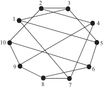
Random regular networks can be used to model social networks in which all individuals have identical numbers of contacts. Observe that the total number of edges is |E(G)| = Nr/2. Thus, the network can be constructed only if Nr is even.
There is no natural probabilistic generation procedure of random regular graphs as in the G(N, p) random graph where the generation algorithm creates each possible edge independently with probability p. One of the standard approaches for constructing the graph is the configuration model proposed by Bender and Cranfield (1978). This model operates as follows. First, generate n points that constitute the vertices of the graph. To each vertex, attach r stubs, which serve as ends of edges. Next, choose pairs of these stubs uniformly at random from two different nodes and join them to make complete edges. The result is a random regular graph G(N, r).
Random regular networks have been used in Kim and Medard (2004) to model resilience issues in large-scale networks. Specifically, it is shown that if r ≥ 3, then G(N, r) is r-connected, which means that for any pair of vertices i and j, there is a path connecting them in every subgraph obtained by deleting r – 1 vertices other than i and j together with their adjacent edges from the graph.
10.6 CONSENSUS OVER RANDOM NETWORKS
Consensus algorithms are used in a wide range of applications, such as load balancing in distributed and parallel computation, and sensor networks. They have also been used as models of opinion dynamics and belief formation in social networks. The central focus of these algorithms is to study whether a group of agents, each of whom has an estimate of an unknown parameter, can reach a global agreement on a common value of the parameter. These agents may engage in information exchange operation such that when agents are made aware of each others’ estimates, they may modify their own estimate by taking into account the opinion of other agents. It is assumed that the agents are interconnected by a network in which the agents are the nodes and an edge exists between two nodes i and j if and only if they can exchange information. Thus, by consensus we mean a situation where all agents agree on a common value of the parameter; that is, xi = xj for all i and j, where xi is some parameter available at node i.
With respect to load balancing, the nodes are processors and two nodes i and j are interconnected by an edge if i can send data to j and vice versa. The measurement xi at node i is the number of jobs the node has to accomplish. To speed up a computation, the nodes exchange information on the xi along the available edges in order to balance the xi as much as possible among the nodes.
With respect to sensor networks, the nodes are sensors that are deployed in a geographical area, and they communicate with other sensors in the area over a wireless medium. The quantities xi that the nodes aim to average can be the measurements taken by each node, which need to be done in order to increase precision by filtering out the noise.
Consider a system of n nodes labeled 1, 2, … , n that are interconnected by a network. Each node i at time k holds a value xi(k). Let x(k) = [x1(k), x2(k), … , xn(k)]T. The interconnection topology of the nodes is represented by a graph in which an edge exists between two nodes if and only if they can exchange information. Let N(i, k) denote the set of nodes that are neighbors of node i at time k. At every time step k, each node i updates its value according to the following equation:
![]()
where wij(k) is the weight that node i assigns to the value of node j, which, as stated earlier, reflects the reliability that node i places in the information from node j. We have that:
![]()
If we define the matrix W(k) whose elements are wij(k), then the system evolves according to the following equation:
![]()
W(k) is called the consensus matrix. A consensus is formed when all the entries of x(k) converge to a common value. That is, the system reaches consensus in probability if, for any initial state x(0) and any ε > 0,
![]()
as k → ∞ for all i, j = 1, … , n. This is a weak form of reaching a consensus. A stronger form is reaching a consensus almost surely, which is that for any initial state x(0),
![]()
as k → ∞ for all i, j = 1, … , n.
To further motivate the discussion, we first consider consensus over a fixed network and then discuss consensus over a random network.
10.6.1 Consensus over Fixed Networks
One of the simplest models of consensus over fixed networks is that proposed by DeGroot (1974). In this model, each node i starts with an initial probability pi(0), which can be regarded as the probability that a given statement is true. Let p(0) = [p1(0), p2(0), … , pn(0)]T. The n × n consensus matrix W(k) has elements wij(k) that represent the weight or trust that node i places on the current belief of node j in forming node i’s belief for the next period. In particular, W(k) is a stochastic matrix that does not depend on k so that we may write W(k) = W. Beliefs are updated over time as follows:
![]()
Solving this equation recursively we obtain:
![]()
Thus, the algorithm is as follows: Every node runs a first-order linear dynamical system to update its estimation using the consensus matrix W and the initial probability vector p(0). The updating process converges to a well-defined limit if ![]() exists for all p(0), which is true if W is an irreducible and aperiodic
matrix. Thus, any closed group of nodes reaches a consensus if the consensus matrix W is irreducible and aperiodic.
exists for all p(0), which is true if W is an irreducible and aperiodic
matrix. Thus, any closed group of nodes reaches a consensus if the consensus matrix W is irreducible and aperiodic.
Example 10.1:
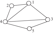
Consider the three-node network shown in Figure 10.7 where the transition probabilities are the wij. The network can be interpreted as follows. Agent 1 weighs all estimates equally; agent 2 weighs its own estimate and that of agent 1 equally and ignores that of agent 3; and agent 3 weighs its own estimate equally with the combined estimates of agents 1 and 2.
Figure 10.7 Figure for Example 10.1.

Since the consensus matrix,
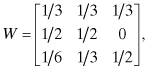
is an irreducible and aperiodic Markov chain, the limits ![]() exist and are independent of the initial distribution, where:
exist and are independent of the initial distribution, where:

Assume that p(0) = [1, 0, 0]T. Thus, we have that:

The solution to this system of equations is:
![]()
Thus,

That is, all three nodes will converge on the same value of pi(k) as k → ∞, which is 9/25.
10.6.1.1 Time to Convergence in a Fixed Network
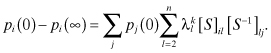
We have discussed the condition for the convergence of a consensus algorithm in a fixed network. However, sometimes it is important to know the time to convergence of an algorithm. To do this we need to know how the opinions at time k, p(k) = Wkp(0), differ from the limiting opinions, p(∞) = W∞p(0). One of the ways we can keep track of this difference is by tracking the difference between Wk and W∞. To do this, we use the diagonalization method that gives:

where S is the matrix whose columns are the eigenvectors of W, and Λ is the diagonal matrix of the corresponding eigenvalues of W. The eigenvalues λ of W satisfy the equation:
![]()
where λ = [λ1, λ2, … , λn]. Let Xi be the eigenvector associated with λi. Then we have that:

and

The Perron–Frobenius theorem states that for an aperiodic and irreducible stochastic matrix P, 1 is a simple eigenvalue and all other eigenvalues have absolute values that are less than 1. Moreover, the left eigenvector X1 corresponding to eigenvalue 1 can be chosen to have all the positive entries and thus can be chosen to be a probability vector by multiplying with an appropriate constant. Thus, for the equation p(k) = Wkp(0), we have that:

From this we obtain:
This means that the convergence of Wk to W∞ depends on how quickly ![]() goes to zero, since |λ2| is the second largest eigenvalue.
goes to zero, since |λ2| is the second largest eigenvalue.
10.6.2 Consensus over Random Networks
Consensus over fixed networks assumes that the network topology is fixed. A variant of the problem is when either the topology of the network or the parameters of the consensus algorithm can randomly change over time. In this section we consider the case where the network topology changes over time. This model has been analyzed in Hatano and Meshahi (2005) and in Tahbaz-Salehi and Jadbabaie (2008).
To deal with the case where the network topology changes over time, we consider the set of possible graphs that can be generated among the n nodes. Each such graph will be referred to as an interaction graph. Assume that there is a set of interaction graphs, which are labeled G1, G2, … , and let G = {G1, G2, … } denote the set of interaction graphs. We assume that the choice of graph Gi at any time step k is made independently with probability pi. Let the consensus matrix corresponding to graph Gi be Wi, and let the set of consensus matrices be W = {W1, W2, … }. Thus, the state x(k) now evolves stochastically, and the convergence of the nodes to the average consensus value will occur in a probabilistic manner. We say that the system reaches a consensus asymptotically on some path ![]() if along the path there exists x* ∈ R such that xi(k) → x* for all i as k → ∞. The value x* is called the asymptotic consensus value.
if along the path there exists x* ∈ R such that xi(k) → x* for all i as k → ∞. The value x* is called the asymptotic consensus value.
Let ![]() be the weight that node i assigns to the value of node j under the interaction graph Gm in time step k, where m = 1, 2, … . Assume that the interaction graphs are used in the order G1, G2, … , Gk in the first k time steps. Then the system evolution,
be the weight that node i assigns to the value of node j under the interaction graph Gm in time step k, where m = 1, 2, … . Assume that the interaction graphs are used in the order G1, G2, … , Gk in the first k time steps. Then the system evolution,
![]()
becomes:
![]()
Thus, in order to check for an asymptotic consensus, we need to investigate the behavior of infinite products of stochastic matrices. Suppose that the average consensus matrix E[W(k)] has n eigenvalues that satisfy the condition:
![]()
In Tahbaz-Salehi and Jadbabaie (2008), it is shown that the discrete dynamical system x(k + 1) = W(k)x(k) reaches state consensus almost surely if |λ2(E[W(k)])| < 1.
10.7 SUMMARY
Complex systems have traditionally been modeled by random graphs that do not produce the topological and structural properties of real networks. Many new network models have been introduced in recent years to capture the scale-free structure of real networks such as the WWW, Internet, biological networks, and social networks. Several properties of these networks have been discussed including average path length, clustering coefficient, and degree distribution. While some complex systems, such as the power grid, can still be modeled by the exponential degree distribution associated with the traditional random graph, others are better modeled by a power-law distribution; sometimes a mixture of exponential and power-law distributions may be used.
The study of complex networks has given rise to a new network science that applies graph theory to the study of dynamic systems that occur in diverse fields. It is an evolving field and the goal of this chapter has been to present its basic principles.
10.8 PROBLEMS
10.1 Consider the graph shown in Figure 10.8.
a. Calculate the diameter of the graph.
b. Obtain the closeness centrality of vertex 1.
c. Obtain the betweenness centrality of vertex 1.
d. Obtain the clustering coefficient of vertex 1.
Figure 10.8 Figure for Problem 10.1.
10.2 Let d(vi) denote the degree of vertex vi of a graph, and let pi be the probability distribution on its vertex set, where:

Using this definition of probability distribution, obtain the entropy of the graph in Figure 10.8.
10.3 Consider a Watts–Strogatz small-world network with lattice radius 3. Calculate the clustering coefficient of the network.
10.4 Calculate the clustering coefficient and the approximate diameter of the random network G(10, 0.3).
10.5 Use the configuration model to generate three instances of the random regular network G(8, 4).