
2
OVERVIEW OF STOCHASTIC PROCESSES
2.1 INTRODUCTION
Stochastic processes deal with the dynamics of probability theory. The concept of stochastic processes enlarges the random variable concept to include time. Thus, instead of thinking of a random variable X that maps an event w ∈ Ω, where Ω is the sample space, to some number X(w), we think of how the random variable maps the event to different numbers at different times. This implies that instead of the number X(w) we deal with X(t, w), where t ∈ T and T is called the parameter set of the process and is usually a set of times.
Stochastic processes are widely encountered in such fields as communications, control, management science, and time series analysis. Examples of stochastic processes include the population growth, the failure of equipment, the price of a given stock over time, and the number of calls that arrive at a switchboard.
If we fix the sample point w, we obtain X(t), which is some real function of time; and for each w, we have a different function X(t). Thus, X(t, w) can be viewed as a collection of time functions, one for each sample point w. On the other hand, if we fix t, we have a function X(w) that depends only on w and thus is a random variable. Thus, a stochastic process becomes a random variable when time is fixed at some particular value. With many values of t we obtain a collection of random variables. Thus, we can define a stochastic process as a family of random variables {X(t, w)|t ∈ T, w ∈ Ω} defined over a given probability space and indexed by the time parameter t. A stochastic process is also called a random process. Thus, we will use the terms “stochastic process” and “random process” interchangeably.
2.2 CLASSIFICATION OF STOCHASTIC PROCESSES
A stochastic process can be classified according to the nature of the time parameter and the values that X(t, w) can take on. As discussed earlier, T is called the parameter set of the random process. If T is an interval of real numbers and hence is continuous, the process is called a continuous-time stochastic process. Similarly, if T is a countable set and hence is discrete, the process is called a discrete-time random process. A discrete-time stochastic process is also called a random sequence, which is denoted by {X[n] n = 1, 2, … }.
The values that X(t, w) assumes are called the states of the stochastic process. The set of all possible values of X(t, w) forms the state space, S, of the stochastic process. If S is continuous, the process is called a continuous-state stochastic process. Similarly, if S is discrete, the process is called a discrete-state stochastic process. In the remainder of this book we denote a stochastic process by X(t), suppressing the parameter w.
2.3 STATIONARY RANDOM PROCESSES
There are several ways to define a stationary random process. At a high level, it is a process whose statistical properties do not vary with time. In this book we consider only two types of stationary processes. These are the strict-sense stationary processes and the wide-sense stationary (WSS) processes.
2.3.1 Strict-Sense Stationary Processes
A random process is defined to be a strict-sense stationary process if its cumulative distribution function (CDF) is invariant to a shift in the time origin. This means that the process X(t) with the CDF FX(x1, x2, … , xn; t1, t2, … , tn) is a strict-sense stationary process if its CDF is identical to that of X(t + ε) for any arbitrary ε. Thus, we have that being a strict-sense stationary process implies that for any arbitrary ε,
![]()
When the CDF is differentiable, the equivalent condition for strict-sense stationarity is that the probability density function (PDF) is invariant to a shift in the time origin; that is,
![]()
If X(t) is a strict-sense stationary process, then the CDF ![]() does not depend on t but it may depend on τ. Thus, if t2 = t1 + τ, then
does not depend on t but it may depend on τ. Thus, if t2 = t1 + τ, then ![]() may depend on t2 – t1, but not on t1 and t2 individually. This means that if X(t) is a strict-sense stationary process, then the autocorrelation and autocovariance functions do not depend on t. Thus, we have that for all τ ∈ T:
may depend on t2 – t1, but not on t1 and t2 individually. This means that if X(t) is a strict-sense stationary process, then the autocorrelation and autocovariance functions do not depend on t. Thus, we have that for all τ ∈ T:

If the condition μX(t) = μX(0) holds for all t, the mean is constant and denoted by μX. Similarly, if the equation RXX(t, t + τ) does not depend on t but is a function of τ, we write RXX(0, τ) = RXX(τ). Finally, whenever the condition CXX(t, t + τ) = CXX(0, τ) holds for all t, we write CXX(0, τ) = CXX(τ).
2.3.2 WSS Processes
Many practical problems that we encounter require that we deal with only the mean and autocorrelation function of a random process. Solutions to these problems are simplified if these quantities do not depend on absolute time. Random processes in which the mean and autocorrelation function do not depend on absolute time are called WSS processes. Thus, for a WSS process X(t),
![]()
Note that a strict-sense stationary process is also a WSS process. However, in general the converse is not true; that is, a WSS process is not necessarily stationary in the strict sense.
2.4 COUNTING PROCESSES
A random process {X(t)|t ≥ 0} is called a counting process if X(t) represents the total number of “events” that have occurred in the interval [0, t). An example of a counting process is the number of customers that arrive at a bank from the time the bank opens its doors for business until some time t. A counting process satisfies the following conditions:
1. X(t) ≥ 0, which means that it has nonnegative values.
2. X(0) = 0, which means that the counting of events begins at time 0.
3. X(t) is integer valued.
4. If s < t, then X(s) ≤ X(t), which means that it is a nondecreasing function of time.
5. X(t) – X(s) represents the number of events that have occurred in the interval [s, t].
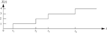
Figure 2.1 represents a sample path of a counting process. The first event occurs at time t1, and subsequent events occur at times t2, t3, and t4. Thus, the number of events that occur in the interval [0, t4] is 4.
Figure 2.1 Sample function of a counting process.
2.5 INDEPENDENT INCREMENT PROCESSES
A counting process is defined to be an independent increment process if the number of events that occur in disjoint time intervals is an independent random variable. For example, in Figure 2.1, consider the two nonoverlapping (i.e., disjoint) time intervals [0, t1] and [t2, t4]. If the number of events occurring in one interval is independent of the number of events that occur in the other, then the process is an independent increment process. Thus, X(t) is an independent increment process if for every set of time instants t0 = 0 < t1 < t2 < … < tn the increments X(t1) – X(t0), X(t2) – X(t1), … , X(tn) – X(tn–1) are mutually independent random variables.
2.6 STATIONARY INCREMENT PROCESS
A counting process X(t) is defined to possess stationary increments if for every set of time instants t0 = 0 < t1 < t2 < … < tn the increments X(t1) – X(t0), X(t2) – X(t1), … , X(tn) – X(tn–1) are identically distributed. In general, the mean of an independent increment process X(t) with stationary increments has the form:
![]()
where the constant m is the value of the mean at time t = 1. That is, m = E[X(1)]. Similarly, the variance of an independent increment process X(t) with stationary increments has the form:
![]()
where the constant σ2 is the value of the variance at time t = 1; that is, σ2 = Var[X(1)].
2.7 POISSON PROCESSES
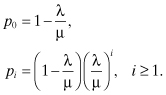
Poisson processes are widely used to model arrivals (or occurrence of events) in a system. For example, they are used to model the arrival of telephone calls at a switchboard, the arrival of customers’ orders at a service facility, and the random failures of equipment. There are two ways to define a Poisson process. The first definition of the process is that it is a counting process X(t) in which the number of events in any interval of length t has a Poisson distribution with mean λt. Thus, for all s, t > 0,
![]()
The second way to define the Poisson process X(t) is that it is a counting process with stationary and independent increments such that for a rate λ > 0, the following conditions hold:
1. P[X(t + Δt) – X(t) = 1] = λΔt + o(Δt), which means that the probability of one event within a small time interval Δt is approximately λΔt, where o(Δt) is a function of Δt that goes to zero faster than Δt does. That is,
![]()
2. P[X(t + Δt) – X(t) ≥ 2] = o(Δt), which means that the probability of two or more events within a small time interval Δt is o(Δt).
3. P[X(t + Δt) – X(t) = 0] = 1 – λΔt + o(Δt).
These three properties enable us to derive the probability mass function (PMF) of the number of events in a time interval of length t as follows:
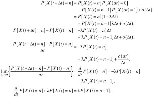
The last equation may be solved iteratively for n = 0, 1, 2, … , subject to the initial conditions:
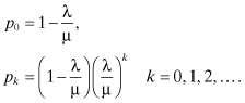
![]()
This gives the PMF of the number of events (or “arrivals”) in an interval of length t as:
![]()
From the results obtained for Poisson random variables earlier in the chapter, we have that:
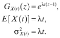
The fact that the mean E[X(t)] = λt indicates that λ is the expected number of arrivals per unit time in the Poisson process. Thus, the parameter λ is called the arrival rate for the process. If λ is independent of time, the Poisson process is called a homogeneous Poisson process. Sometimes the arrival rate is a function of time, and we represent it as λ(t). Such processes are called nonhomogeneous Poisson processes. In this book we are concerned mainly with homogeneous Poisson processes.
Another important property of the Poisson process is that the interarrival times of customers are exponentially distributed with parameter λ. This can be demonstrated by noting that if T is the time until the next arrival, then P[T > t] = P[X(t) = 0] = e–λt. Therefore, the CDF and PDF of the interarrival time are given by:
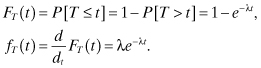
Thus, the time until the next arrival is always exponentially distributed. From the memoryless property of the exponential distribution, the future evolution of the Poisson process is independent of the past and is always probabilistically the same. Therefore, the Poisson process is memoryless. As the saying goes, “the Poisson process implies exponential distribution, and the exponential distribution implies the Poisson process.” The Poisson process deals with the number of arrivals within a given time interval where interarrival times are exponentially distributed, and the exponential distribution measures the time between arrivals where customers arrive according to a Poisson process.
2.8 RENEWAL PROCESSES
Consider an experiment that involves a set of identical light bulbs whose lifetimes are independent. The experiment consists of using one light bulb at a time, and when it fails it is immediately replaced by another light bulb from the set. Each time a failed light bulb is replaced constitutes a renewal event. Let Xi denote the lifetime of the ith light bulb, i = 1, 2, … , where X0 = 0. Because the light bulbs are assumed to be identical, the Xi are independent and identically distributed with PDF fX(x), x ≥ 0, and mean E[X].
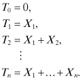
Let N(t) denote the number of renewal events up to and including the time t, where it is assumed that the first light bulb was turned on at time t = 0. The time to failure Tn of the first n light bulbs is given by:
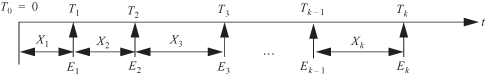
The relationship between the interevent times Xn and the Tn is illustrated in Figure 2.2, where Ek denotes the kth event.
Figure 2.2 Interarrival times of a renewal process.
Tn is called the time of the nth renewal, and we have that:
![]()
Thus, the process {N(t)|t ≥ 0} is a counting process known as a renewal process, and N(t) denotes the number of renewals up to time t. Observe that the event that the number of renewals up to and including the time t is less than n is equivalent to the event that the nth renewal occurs at a time that is later than t. Thus, we have that:
![]()
Therefore, P[N(t) < n] = P[Tn > t]. Let ![]() and
and ![]() denote the PDF and CDF, respectively, of Tn. Thus, we have that:
denote the PDF and CDF, respectively, of Tn. Thus, we have that:
![]()
Because P[N(t) = n] = P[N(t) < n + 1] – P[N(t) < n], we obtain the following result for the PMF of N(t):
![]()
2.8.1 The Renewal Equation
The expected number of renewals by time t is called the renewal function. It is denoted by H(t) and given by:
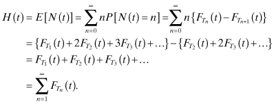
If we take the derivative of each side we obtain:
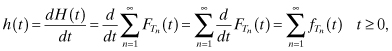
where h(t) is called the renewal density. Let Mh(s) denote the one-sided Laplace transform of h(t) and ![]() the s-transform of
the s-transform of ![]() . Because Tn is the sum of n independent and identically distributed random variables, the PDF
. Because Tn is the sum of n independent and identically distributed random variables, the PDF ![]() is the n-fold convolution of the PDF of X. Thus, we have that
is the n-fold convolution of the PDF of X. Thus, we have that
![]() . From this we obtain Mh(s) as follows:
. From this we obtain Mh(s) as follows:
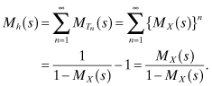
This gives:
![]()
Taking the inverse transform we obtain:
![]()
Finally, integrating both sides of the equation, we obtain:
![]()
This equation is called the fundamental equation of renewal theory.
Example 2.1:
Assume that X is exponentially distributed with mean 1/λ. Then we obtain:
where L−1{Mh(s)} is the inverse Laplace transform of Mh(s).
2.8.2 The Elementary Renewal Theorem
We state the following theorem called the elementary renewal theorem without proof:
![]()
2.8.3 Random Incidence and Residual Time
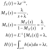
Consider a renewal process N(t) in which events (or arrivals) occur at times 0 = T0, T1, T2, … . As discussed earlier, the interevent times Xk can be defined in terms of the Tk as follows:
Note that the Xk are mutually independent and identically distributed.
Consider the following problem in connection with the Xk. Assume the Tk are the points in time that buses arrive at a bus stop. A passenger arrives at the bus stop at a random time and wants to know how long he or she will wait until the next bus arrival. This problem is usually referred to as the random incidence problem, because the subject (or passenger in this example) is incident to the process at a random time. Let R be the random variable that denotes the time from the moment the passenger arrived until the next bus arrival. R is referred to as the residual life of the renewal process. Also, let W denote the length of the interarrival gap that the passenger entered by random incidence. Figure 2.3 illustrates the random incidence problem.
Figure 2.3 Random incidence.

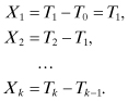
Let fX(x) denote the PDF of the interarrival times; let fW(w) denote the PDF of W, the gap entered by random incidence; and let fR(r) denote the PDF of the residual life, R. The probability that the random arrival occurs in a gap of length between w and w + dw can be assumed to be directly proportional to the length w of the gap and relative occurrence fX(w)dw of such gaps. That is,
![]()
where β is a constant of proportionality. Thus, fW(w) = βwfX(w). Because fW(w) is a PDF, we have that:
![]()
Thus, β = 1/E[X], and we obtain:
![]()
The expected value of W is given by E[W] = E[X2]/E[X]. This result applies to all renewal processes.
A Poisson process is an example of a renewal process in which X is exponentially distributed with E[X] = 1/λ and E[X2] = 2/λ2. Thus, for a Poisson process we obtain:
![]()
This means that for a Poisson process the gap entered by random incidence has the second-order Erlang distribution; thus, the expected length of the gap is twice the expected length of an interarrival time. This is often referred to as the random incidence paradox. The reason for this fact is that the passenger is more likely to enter a large gap than a small gap; that is, the gap entered by random incidence is not a typical interval.
Next, we consider the PDF of the residual life R of the process. Given that the passenger enters a gap of length w, he or she is equally likely to be anywhere within the gap. Thus, the conditional PDF of R, given that W = w, is given by:
![]()
When we combine this result with the previous one, we get the joint PDF of R and W as follows:

The marginal PDF of R and its expected value become:
For the Poisson process, X is exponentially distributed and 1 – FX(r) = e–λr, which means that:
![]()
Thus, for a Poisson process, the residual life of the process has the same distribution as the interarrival time, which can be expected from the “forgetfulness” property of the exponential distribution.
In Figure 2.3, the random variable V denotes the time between the last bus arrival and the passenger’s random arrival. Because W = V + R, the expected value of V is:
![]()
2.9 MARKOV PROCESSES
Markov processes are widely used in engineering, science, and business modeling. They are used to model systems that have a limited memory of their past. For example, consider a sequence of games where a player gets $1 if he wins a game and loses $1 if he loses the game. Then the amount of money the player will make after n + 1 games is determined by the amount of money he has made after n games. Any other information is irrelevant in making this prediction. In population growth studies, the population of the next generation depends mainly on the current population and possibly the last few generations.
A random process {X(t)|t ∈ T} is called a first-order Markov process if for any t0 < t1 < … < tn the conditional CDF of X(tn) for given values of X(t0), X(t1), … , X(tn–1) depends only on X(tn–1). That is,
![]()
This means that, given the present state of the process, the future state is independent of the past. This property is usually referred to as the Markov property. In second-order Markov processes, the future state depends on both the current state and the last immediate state, and so on for higher order Markov processes. In this chapter we consider only first-order Markov processes.
Markov processes are classified according to the nature of the time parameter and the nature of the state space. With respect to state space, a Markov process can be either a discrete-state Markov process or a continuous-state Markov process. A discrete-state Markov process is called a Markov chain. Similarly, with respect to time, a Markov process can be either a discrete-time Markov process or a continuous-time Markov process. Thus, there are four basic types of Markov processes (Ibe 2009):
1. Discrete-time Markov chain (or discrete-time discrete-state Markov process)
2. Continuous-time Markov chain (or continuous-time discrete-state Markov process)
3. Discrete-time Markov process (or discrete-time continuous-state Markov process)
4. Continuous-time Markov process (or continuous-time continuous-state Markov process)
This classification of Markov processes is illustrated in Figure 2.4.
Figure 2.4 Classification of Markov processes.

2.9.1 Discrete-Time Markov Chains
The discrete-time process {Xk, k = 0, 1, 2, … } is called a Markov chain if for all i, j, k, … , m, the following is true:
![]()
The quantity pijk is called the state transition probability, which is the conditional probability that the process will be in state j at time k immediately after the next transition, given that it is in state i at time k – 1. A Markov chain that obeys the preceding rule is called a nonhomogeneous Markov chain. In this book we will consider only homogeneous Markov chains, which are Markov chains in which pijk = pij. This means that homogeneous Markov chains do not depend on the time unit, which implies that:
![]()
which is the so-called Markov property. The homogeneous state transition probability pij satisfies the following conditions:
1. 0 ≤ pij ≤ 1
2.
![]() which follows from the fact that the states are
mutually exclusive and collectively exhaustive.
which follows from the fact that the states are
mutually exclusive and collectively exhaustive.
From the above definition we obtain the following Markov chain rule:

Thus, once we know the initial state X0 we can evaluate the joint probability P[Xk, Xk–1, … , X0].
2.9.1.1 State Transition Probability Matrix
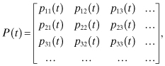
It is customary to display the state transition probabilities as the entries of an n × n matrix P, where pij is the entry in the ith row and jth column:
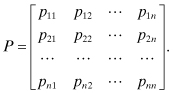
P is called the transition probability matrix. It is a stochastic matrix because for any row i, ![]()
2.9.1.2 The n-Step State Transition Probability
Let pij(n) denote the conditional probability that the system will be in state j after exactly n transitions, given that it is currently in state i. That is,
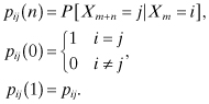
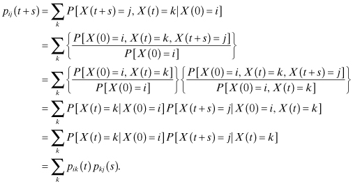
Consider the two-step transition probability pij(2), which is defined by:
![]()
Assume that m = 0, then:
where the second to the last equality is due to the Markov property. The final equation states that the probability of starting in state i and being in state j at the end of the second transition is the probability that we first go immediately from state i to some intermediate state k and then immediately from state k to state j; the summation is taken over all possible intermediate states k.
Proposition:
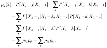
The following proposition deals with a class of equations called the Chapman–Kolmogorov equations, which provide a generalization of the above results obtained for the two-step transition probability. For all 0 < r < n,
![]()
This proposition states that the probability that the process starts in state i and finds itself in state j at the end of the nth transition is the product of the probability that the process starts in state i and finds itself in some intermediate state k after r transitions and the probability that it goes from state k to state j after additional n – r transitions.
Proof:
The proof is a generalization of the proof for the case of n = 2 and is as follows:
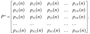
From the preceding discussion it can be shown that pij(n) is the ijth entry (ith row, jth column) in the matrix Pn. That is, for an N-state Markov chain, Pn is the matrix:
2.9.1.3 State Transition Diagrams
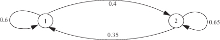
Consider the following problem. It has been observed via a series of tosses of a particular biased coin that the outcome of the next toss depends on the outcome of the current toss. In particular, given that the current toss comes up heads, the next toss will come up heads with probability 0.6 and tails with probability 0.4. Similarly, given that the current toss comes up tails, the next toss will come up heads with probability 0.35 and tails with probability 0.65.
If we define state 1 to represent heads and state 2 to represent tails, then the transition probability matrix for this problem is the following:
![]()
All the properties of the Markov process can be determined from this matrix. However, the analysis of the problem can be simplified by the use of the state transition diagram in which the states are represented by circles and directed arcs represent transitions between states. The state transition probabilities are labeled on the appropriate arcs. Thus, with respect to the above problem, we obtain the state transition diagram shown in Figure 2.5.
Figure 2.5 Example of a state transition diagram.
Example 2.2:
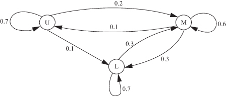
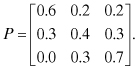
Assume that people in a particular society can be classified as belonging to the upper class (U), middle class (M), and lower class (L). Membership in any class is inherited in the following probabilistic manner. Given that a person is raised in an upper-class family, he or she will have an upper-class family with probability 0.7, a middle-class family with probability 0.2, and a lower-class family with probability 0.1. Similarly, given that a person is raised in a middle-class family, he or she will have an upper-class family with probability 0.1, a middle-class family with probability 0.6, and a lower-class family with probability 0.3. Finally, given that a person is raised in a lower-class family, he or she will have a middle-class family with probability 0.3 and a lower-class family with probability 0.7. Determine (a) the transition probability matrix and (b) the state transition diagram for this problem.
Solution:
(a) Using the first row to represent the upper class, the second row to represent the middle class, and the third row to represent the lower class, we obtain the following transition probability matrix:
(b) The state transition diagram is as shown in Figure 2.6.
Figure 2.6 State transition diagram for Example 2.2.
2.9.1.4 Classification of States
A state j is said to be accessible (or can be reached) from state i if, starting from state i, it is possible that the process will ever enter state j. This implies that pij(n) > 0 for some n > 0. Thus, the n-step probability enables us to obtain reachability information between any two states of the process.
Two states that are accessible from each other are said to communicate with each other. The concept of communication divides the state space into different classes. Two states that communicate are said to be in the same class. All members of one class communicate with one another. If a class is not accessible from any state outside the class, we define the class to be a closed communicating class. A Markov chain in which all states communicate, which means that there is only one class, is called an irreducible Markov chain. For example, the Markov chains shown in Figures 2.5 and 2.6 are irreducible Markov chains.
The states of a Markov chain can be classified into two broad groups: those that the process enters infinitely often and those that it enters finitely often. In the long run, the process will be found to be in only those states that it enters infinitely often. Let fij(n) denote the conditional probability that given that the process is presently in state i, the first time it will enter state j occurs in exactly n transitions (or steps). We call fij(n) the probability of first passage from state i to state j in n transitions. The parameter fij, which is defined as follows,

is the probability of first passage from state i to state j. It is the conditional probability that the process will ever enter state j, given that it was initially in state i. Obviously fij(1) = pij and a recursive method of computing fij(n) is:
![]()
The quantity fii denotes the probability that a process that starts at state i will ever return to state i. Any state i for which fii = 1 is called a recurrent state, and any state i for which fii < 1 is called a transient state. More formally, we define these states as follows:
a. A state j is called a transient (or nonrecurrent) state if there is a positive probability that the process will never return to j again after it leaves j.
b. A state j is called a recurrent (or persistent) state if, with probability 1, the process will eventually return to j after it leaves j. A set of recurrent states forms a single chain if every member of the set communicates with all other members of the set.
c. A recurrent state j is called a periodic state if there exists an integer d, d > 1, such that pjj(n) is zero for all values of n other than d, 2d, 3d, … ; d is called the period. If d = 1, the recurrent state j is said to be aperiodic.
d. A recurrent state j is called a positive recurrent state if, starting at state j, the expected time until the process returns to state j is finite. Otherwise, the recurrent state is called a null recurrent state.
e. Positive recurrent, aperiodic states are called ergodic states.
f. A chain consisting of ergodic states is called an ergodic chain.
g. A state j is called an absorbing (or trapping) state if pjj = 1. Thus, once the process enters a trapping or absorbing state, it never leaves the state, which means that it is “trapped.”
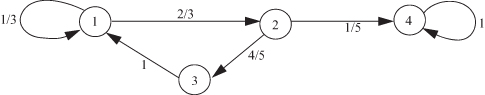
Example 2.3:
Consider the Markov chain with the state transition diagram shown in Figure 2.7. State 4 is a transient state while states 1, 2, and 3 are recurrent states. There is no periodic state, and there is one chain, which is {1, 2, 3}.
Figure 2.7 State transition diagram for Example 2.3.

Example 2.4:
Consider the state transition diagram of Figure 2.8, which is a modified version of Figure 2.7. Here, the transition is now from state 2 to state 4 instead of from state 4 to state 2. For this case, states 1, 2, and 3 are now transient states because when the process enters state 2 and makes a transition to state 4, it does not return to these states again. Also, state 4 is a trapping (or absorbing) state because once the process enters the state, the process never leaves the state. As stated in the definition, we identify a trapping state by the fact that, as in this example, p44 = 1 and p4k = 0 for k not equal to 4.
Figure 2.8 State transition diagram for Example 2.4.
2.9.1.5 Limiting State Probabilities
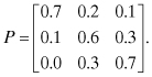
Recall that the n-step state transition probability pij(n) is the conditional probability that the system will be in state j after exactly n transitions, given that it is presently in state i. The n-step transition probabilities can be obtained by multiplying the transition probability matrix by itself n times. For example, consider the following transition probability matrix:
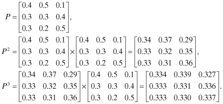
From the matrix P2 we obtain the pij(2). For example, p23(2) = 0.35, which is the entry in the second row and third column of the matrix P2 . Similarly, the entries of the matrix P3 are the pij(3).
For this particular matrix and matrices for a large number of Markov chains, we find that as we multiply the transition probability matrix by itself many times, the entries remain constant. More importantly, all the members of one column will tend to converge to the same value.
If we define P[X(0) = i] as the probability that the process is in state i before it makes the first transition, then the set {P[X(0) = i]} defines the initial condition for the process, and for an N-state process,
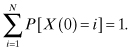
Let P[X(n) = j] denote the probability that the process is in state j at the end of the first n transitions, then for the N-state process,
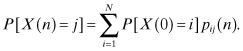
For the class of Markov chains referenced above, it can be shown that as n → ∞, the n-step transition probability pij(n) does not depend on i, which means that P[X(n) = j] approaches a constant as n → ∞ for this class of Markov chains. That is, the constant is independent of the initial conditions. Thus, for the class of Markov chains in which the limit exists, we define the limiting state probabilities as follows:
![]()
Recall that the n-step transition probability can be written in the form:
![]()
If the limiting state probabilities exist and do not depend on the initial state, then:
![]()
If we define the limiting state probability vector π = [π1, π2, … , πN ], then we have that:

where the last equation is due to the law of total probability. Each of the first two equations, together with the last equation, gives a system of linear equations that the πj must satisfy. The following propositions specify the conditions for the existence of the limiting state probabilities:
a.
In any irreducible, aperiodic Markov chain, the limits ![]() exist
and are independent of the initial distribution.
exist
and are independent of the initial distribution.
b.
In any irreducible, periodic Markov chain the limits ![]() exist
and are independent of the initial distribution. However, they must be interpreted as the long-run probability that the process is in state j.
exist
and are independent of the initial distribution. However, they must be interpreted as the long-run probability that the process is in state j.
Example 2.5:
Recall the biased coin problem whose state transition diagram is given in Figure 2.5 and reproduced in Figure 2.9. Suppose we are required to find the limiting state probabilities. We proceed as follows. There are three equations associated with the above Markov chain, and they are:
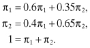
Figure 2.9 State transition diagram for Example 2.5.

Since there are three equations and two unknowns, one of the equations is redundant. Thus, the rule of thumb is that for an N-state Markov chain, we use the first N – 1 linear equations from the relation ![]() and the law
of total probability:
and the law
of total probability: ![]() . For the given problem we have:
. For the given problem we have:
![]()
From the first equation, we obtain π1 = (0.35/0.4)π2 = (7/8)π2. Substituting for π1 and solving for π2 in the second equation, we obtain the result π = {π1, π2} = {7/15, 8/15}.
Suppose we are also required to compute p12(3), which is the probability that the process will be in state 2 at the end of the third transition, given that it is presently in state 1. We can proceed in two ways: the direct method and the matrix method. We consider both methods.
a. Direct Method: Under this method we exhaustively enumerate all the possible ways of a state 1-to-state 2 transition in three steps. If we use the notation a → b → c to denote a transition from state a to state b and then from state b to state c, the desired result is the following:
![]()
Since the different events are mutually exclusive, we obtain:

b. Matrix Method: One of the limitations of the direct method is that it is difficult to exhaustively enumerate the different ways of going from state 1 to state 2 in n steps, especially when n is large. This is where the matrix method becomes very useful. As discussed earlier, pij(n) is the ijth entry in the matrix Pn. Thus, for the current problem, we are looking for the entry in the first row and second column of the matrix P3. Therefore, we have:
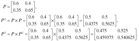
The required result (first row, second column) is 0.525, which is the result obtained via the direct method.
2.9.1.6 Doubly Stochastic Matrix
A transition probability matrix P is defined to be a doubly stochastic matrix if each of its columns sums to 1. That is, not only does each row sum to 1, each column also sums to 1. Thus, for every column j of a doubly stochastic matrix, we have that ![]() .
.
Doubly stochastic matrices have interesting limiting state probabilities, as the following theorem shows.
Theorem:
If P is a doubly stochastic matrix associated with the transition probabilities of a Markov chain with N states, then the limiting state probabilities are given by πi = 1/N, i = 1, 2, … , N.
Proof:
We know that the limiting state probabilities satisfy the condition:
![]()
To check the validity of the theorem, we observe that when we substitute πi = 1/N, i = 1, 2, … , N, in the above equation we obtain:
![]()
This shows that πi = 1/N satisfies the condition π = πP, which the limiting state probabilities are required to satisfy. Conversely, from the above equation, we see that if the limiting state probabilities are given by 1/N, then each column j of P sums to 1; that is, P is doubly stochastic. This completes the proof.
Example 2.6:
Find the transition probability matrix and the limiting state probabilities of the process represented by the state transition diagram shown in Figure 2.10.
Figure 2.10 State transition diagram for Example 2.6.
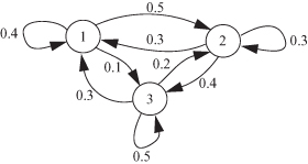
Solution:
The transition probability matrix is given by:
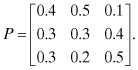
It can be seen that each row of the matrix sums to 1 and each column also sums to 1; that is, it is a doubly stochastic matrix. Since the process is an irreducible, aperiodic Markov chain, the limiting state probabilities exist and are given by π1 = π2 = π3 = 1/3.
2.9.2 Continuous-Time Markov Chains
A random process {X(t)|t ≥ 0} is a continuous-time Markov chain if, for all s, t ≥ 0 and nonnegative integers i, j, k,
![]()
This means that in a continuous-time Markov chain, the conditional probability of the future state at time t + s given the present state at s and all past states depends only on the present state and is independent of the past. If, in addition P[X(t + s) = j|X(s) = i] is independent of s, then the process {X(t)|t ≥ 0} is said to be time homogeneous or have the time homogeneity property. Time-homogeneous Markov chains have stationary (or homogeneous) transition probabilities. Let:
![]()
That is, pij(t) is the probability that a Markov chain that is presently in state i will be in state j after an additional time t, and pj(t) is the probability that a Markov chain is in state j at time t. Thus, the pij(t) are the transition probability functions that satisfy the following condition:
![]()
Also,
![]()
which follows from the fact that at any given time the process must be in some state. Also,
This equation is called the Chapman–Kolmogorov equation for the continuous-time Markov chain. Note that the second to last equation is due to the Markov property. If we define P(t) as the matrix of the pij(t), that is,
then the Chapman–Kolmogorov equation becomes:
![]()
Whenever a continuous-time Markov chain enters a state i, it spends an amount of time called the dwell time (or holding time) in that state. The holding time in state i is exponentially distributed with mean 1/νi. At the expiration of the holding time, the process makes a transition to another state j with probability pij, where:
![]()
Because the mean holding time in state i is 1/νi, νi represents the rate at which the process leaves state i and νipij represents the rate when in state i that the process makes a transition to state j. Also, since the holding times are exponentially distributed, the probability that when the process is in state i a transition to state j ≠ i will take place in the next small time Δt is pijνi Δt. The probability that no transition out of state i will take place in Δt given that the process is presently in state i is ![]() , and
, and ![]() is the probability that it leaves state i in Δt.
is the probability that it leaves state i in Δt.
With these definitions, we consider the state transition diagram for the process, which is shown in Figure 2.11 for state i. We consider the transition equations for state i for the small time interval Δt.
Figure 2.11 State transition diagram for state i over small time Δt.
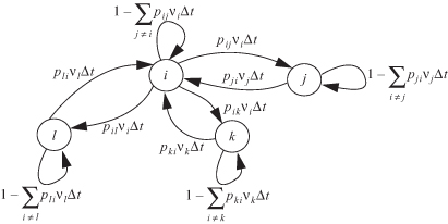
From Figure 2.11, we obtain the following equation:
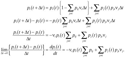
In the steady state, pj(t) → pj and:
![]()
Thus, we obtain:
Alternatively, we may write:
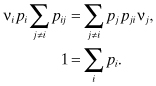
The left side of the first equation is the rate of transition out of state i, while the right side is the rate of transition into state i. This “balance” equation states that in the steady state the two rates are equal for any state in the Markov chain.
2.9.2.1 Birth and Death Processes
Birth and death processes are a special type of continuous-time Markov chains. Consider a continuous-time Markov chain with states 0, 1, 2, … . If pij = 0 whenever j ≠ i – 1 or j ≠ i + 1, then the Markov chain is called a birth and death process. Thus, a birth and death process is a continuous-time Markov chain with states 0, 1, 2, … , in which transitions from state i can only go to either state i + 1 or state i – 1. That is, a transition either causes an increase in state by 1 or a decrease in state by 1. A birth is said to occur when the state increases by 1, and a death is said to occur when the state decreases by 1. For a birth and death process, we define the following transition rates from state i:
![]()
Thus, λi is the rate at which a birth occurs when the process is in state i and μi is the rate at which a death occurs when the process is in state i. The sum of these two rates is λi + μi = νi, which is the rate of transition out of state i. The state transition rate diagram of a birth and death process is shown in Figure 2.12. It is called a state transition rate diagram as opposed to a state transition diagram because it shows the rate at which the process moves from state to state and not the probability of moving from one state to another. Note that μ0 = 0, since there can be no death when the process is in an empty state.
Figure 2.12 State transition rate diagram for the birth and death process.
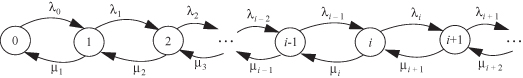
The actual state transition probabilities when the process is in state i are pi(i+1) and pi(i–1). By definition, pi(i+1) = λi/(λi + μi) is the probability that a birth occurs before a death when the process is in state i. Similarly, pi(i–1) = μi/(λi + μi) is the probability that a death occurs before a birth when the process is in state i.
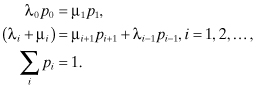
Recall that the rate at which the probability of the process being in state i changes with time is given by:
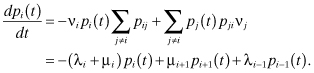
Thus, for the birth and death process we have that:
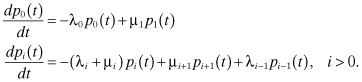
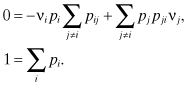
In the steady state,
![]()
If we assume that the limiting probabilities ![]() exist, then from
the above equation we obtain the following:
exist, then from
the above equation we obtain the following:

The equation states that the rate at which the process leaves state i either through a birth or a death is equal to the rate at which it enters the state through a birth when the process is in state i – 1 or through a death when the process is in state i + 1. This is called the balance equation because it balances (or equates) the rate at which the process enters state i with the rate at which it leaves state i.
Example 2.7:
A machine is operational for an exponentially distributed time with mean 1/λ before breaking down. When it breaks down, it takes a time that is exponentially distributed with mean 1/µ to repair it. What is the fraction of time that the machine is operational (or available)?
Solution:
This is a two-state birth and death process. Let U denote the up state and D the down state. Then, the state transition rate diagram is shown in Figure 2.13.
Figure 2.13 State transition rate diagram for Example 2.7.
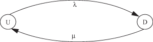
Let pU denote the steady-state probability that the process is in the operational state, and let pD denote the steady-state probability that the process is in the down state. Then the balance equations become:
![]()
Substituting pD = 1 – pU in the first equation gives pU = μ/(λ + μ).
Example 2.8:
Customers arrive at a bank according to a Poisson process with rate λ. The time to serve each customer is exponentially distributed with mean 1/µ. There is only one teller at the bank, and an arriving customer who finds the teller busy when she arrives will join a single queue that operates on a first-come, first-served basis. Determine the limiting state probabilities given that μ > λ.
Solution:
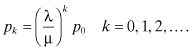
This is a continuous-time Markov chain in which arrivals constitute births and service completions constitute deaths. Also, for all i, μi = μ and λi = λ. Thus, if pk denotes the steady-state probability that there are k customers in the system, the balance equations are as follows:
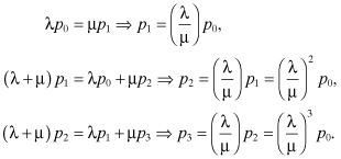
Similarly, it can be shown that:
Now,

Thus,
2.9.2.2 Local Balance Equations
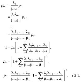
Recall that the steady-state solution of the birth and death process is given by:
For i = 1, we obtain (λ1 + μ1) p1 = μ2p2 + λ0p0. Since we know from the first equation that λ0 p0 = μ1p1, this equation becomes:
![]()
Similarly, for i = 2, we have that (λ2 + μ2) p2 = μ3p3 + λ1p2. Applying the last result, we obtain:
![]()
Repeated application of this method yields the general result
![]()
This result states that when the process is in the steady state, the rate at which it makes a transition from state i to state i + 1, which we refer to as the rate of flow from state i to state i + 1, is equal to the rate of flow from state i + 1 to state i. This property is referred to as local balance condition. Direct application of the property allows us to solve for the steady-state probabilities recursively as follows:
When λi = λ for all i and μi = μ for all i, we obtain the result:
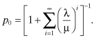
The sum converges if and only if λ/μ < 1, which is equivalent to the condition that λ < μ. Under this condition we obtain the solutions:
In Chapter 3, we will refer to this special case of the birth and death process as an M/M/1 queueing system.
2.10 GAUSSIAN PROCESSES
Gaussian processes are important in many ways. First, many physical problems are the results of adding large numbers of independent random variables. According to the central limit theorem, such sums of random variables are essentially normal (or Gaussian) random variables. Also, the analysis of many systems is simplified if they are assumed to be Gaussian processes because of the properties of Gaussian processes. For example, noise in communication systems is usually modeled as a Gaussian process. Similarly, noise voltages in resistors are modeled as Gaussian processes.
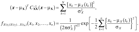
A stochastic process {X(t), t ∈ T} is defined to be a Gaussian process if and only if for any choice of n real coefficients a1, a2, … , an and choice of n time instants t1, t2, … , tn in the index set T, the random variable a1X(t1) + a2X(t2) + … + anX(tn) is a Gaussian (or normal) random variable. That is, {X(t), t ∈ T} is a Gaussian process if any finite linear combination of the X(t) is a normally distributed random variable. This definition implies that the random variables X(t1), X(t2), … , X(tn) have a jointly normal PDF; that is,
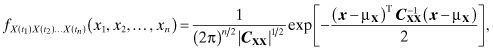
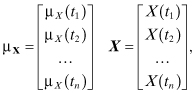
where μX is the vector of the mean functions of the X(tk), CXX is the matrix of the autocovariance functions, X is the vector of the X(tk), and T denotes the transpose operation. That is,

If the X(tk) are mutually uncorrelated, then:
![]()
The autocovariance matrix and its inverse become:
Thus, we obtain
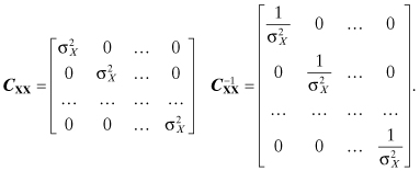
If in addition to being mutually uncorrelated the random variables X(t1), X(t2), … , X(tn) have different variances such that ![]() , (1 ≤ k ≤ n), then the covariance matrix and the joint PDF are given by:
, (1 ≤ k ≤ n), then the covariance matrix and the joint PDF are given by:
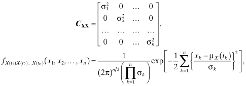
which implies that X(t1), X(t2), … , X(tn) are also mutually independent. We list three important properties of Gaussian processes:
1. A Gaussian process that is a WSS process is also a strict-sense stationary process.
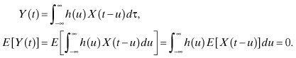
2. If the input to a linear system is a Gaussian process, then the output is also a Gaussian process.
3. If the input X(t) to a linear system is a zero-mean Gaussian process, the output process Y(t) is also a zero-mean process. The proof of this property is as follows:
Example 2.9:
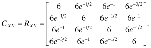
A WSS Gaussian random process has an autocorrelation function:
![]()
Determine the covariance matrix of the random variables X(t), X(t + 1), X(t + 2), and X(t + 3).
Solution:
First, note that:
![]()
Let X1 = X(t), X2 = X(t + 1), X3 = X(t + 2), X4 = X(t + 3). Then the elements of the covariance matrix are given by:
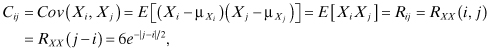
where Rij is the i–jth element of the autocorrelation matrix. Thus,
2.11 PROBLEMS
2.1 Cars arrive from the northbound section of an intersection in a Poisson manner at the rate of λN cars per minute and from the eastbound section in a Poisson manner at the rate of λE cars per minute.
a. Given that there is currently no car at the intersection, what is the probability that a northbound car arrives before an eastbound car?
b. Given that there is currently no car at the intersection, what is the probability that the fourth northbound car arrives before the second eastbound car?
2.2 Suppose X(t) is a Gaussian random process with a mean E[X(t)] = 0 and autocorrelation function RXX(τ) = e–|τ|. Assume that the random variable A is defined as follows:
![]()
Determine the following:
a. E[A]
b.
![]()
2.3 Suppose X(t) is a Gaussian random process with a mean E[X(t)] = 0 and autocorrelation function RXX(τ) = e–|τ|. Assume that the random variable A is defined as follows:
![]()
where B is a uniformly distributed random variable with values between 1 and 5 and is independent of the random process X(t). Determine the following:
a. E[A]
b.
![]()
2.4 Consider a machine that is subject to failure and repair. The time to repair the machine when it breaks down is exponentially distributed with mean 1/µ. The time the machine runs before breaking down is also exponentially distributed with mean 1/λ. When repaired, the machine is considered to be as good as new. The repair time and the running time are assumed to be independent. If the machine is in good condition at time 0, what is the expected number of failures up to time t?
2.5 The Merrimack Airlines company runs a commuter air service between Manchester, New Hampshire, and Cape Cod, Massachusetts. Because the company is a small one, there is no set schedule for their flights, and no reservation is needed for the flights. However, it has been determined that their planes arrive at the Manchester airport according to a Poisson process with an average rate of two planes per hour. Gail arrived at the Manchester airport and had to wait to catch the next flight.
a. What is the mean time between the instant Gail arrived at the airport until the time the next plane arrived?
b. What is the mean time between the arrival time of the last plane that took off from the Manchester airport before Gail arrived and the arrival time of the plane that she boarded?
2.6 Victor is a student who is conducting experiments with a series of light bulbs. He started with 10 identical light bulbs, each of which has an exponentially distributed lifetime with a mean of 200 h. Victor wants to know how long it will take until the last bulb burns out (or fails). At noontime, he stepped out to get some lunch with six bulbs still on. Assume that he came back and found that none of the six bulbs has failed.
a. After Victor came back, what is the expected time until the next bulb failure?
b. What is the expected length of time between the fourth bulb failure and the fifth bulb failure?
2.7 A machine has three components labeled 1, 2, and 3, whose times between failure are exponentially distributed with mean 1/λ1, 1/λ2 and 1/λ3, respectively. The machine needs all three components to work, thus when a component fails the machine is shut down until the component is repaired and the machine is brought up again. When repaired, a component is considered to be as good as new. The time to repair component 1 when it fails is exponentially distributed with mean 1/µ1. The time to repair component 2 when it fails is constant at 1/µ2, and the time to repair component 3 when it fails is a third-order Erlang random variable with parameter μ3.
a. What fraction of time is the machine working?
b. What fraction of time is component 2 being repaired?
c. What fraction of time is component 3 idle but has not failed?
d. Given that Bob arrived when component 1 was being repaired, what is the expected time until the machine is operational again?
2.8 Customers arrive at a taxi depot according to a Poisson process with rate λ. The dispatcher sends for a taxi where there are N customers waiting at the station. It takes M units of time for a taxi to arrive at the depot. When it arrives, the taxi picks up all waiting customers. The taxi company incurs a cost at a rate of nk per unit time whenever n customers are waiting. What is the steady-state average cost that the company incurs?
2.9 Consider a Markov chain with the following transition probability matrix:
a. Give the state transition diagram.
b. Obtain the limiting state probabilities.
c. Given that the process is currently in state 1, what is the probability that it will be in state 2 at the end of the third transition?