
3
ELEMENTARY QUEUEING THEORY
3.1 INTRODUCTION
A queue is a waiting line. Queues arise in many of our daily activities. For example, we join a queue to buy stamps at the post office, to cash checks or deposit money at the bank, to pay for groceries at the grocery store, to purchase tickets for movies or games, or to get a table at the restaurant. This chapter discusses a class of queueing systems called Markovian queueing systems. They are characterized by the fact that either the service times are exponentially distributed or customers arrive at the system according to a Poisson process, or both. The emphasis in this chapter is on the steady-state analysis with limited discussion on transient analysis.
3.2 DESCRIPTION OF A QUEUEING SYSTEM
In a queueing system, customers from a specified population arrive at a service facility to receive service. The service facility has one or more servers who attend to arriving customers. If a customer arrives at the facility when all the servers are busy attending to earlier customers, the arriving customer joins the queue until a server is free. After a customer has been served, he leaves the system and will not join the queue again. That is, service with feedback is not allowed. We consider systems that obey the work conservation rule: A server cannot be idle when there are customers to be served. Figure 3.1 illustrates the different components of a queueing system.
Figure 3.1 Components of a queueing system.

When a customer arrives at a service facility, a server commences service on the customer if the server is currently idle. Otherwise, the customer joins a queue that is attended to in accordance with a specified service policy such as first-come, first-served (FCFS), last-come, first served (LCFS), priority, and so on. Thus, the time a customer spends waiting for service to begin is dependent on the service policy. Also, since there can be one or more servers in the facility, more than one customer can be receiving service at the same time. The following notation is used to represent the random variables associated with a queueing system:
a. Nq is the number of customers in queue, waiting to be served
b. Ns is the number of customers currently receiving service
c. N is the total number of customers in the system: N = Nq + Ns
d. W is the time a customer spends in queue before going to service; W is the waiting time
e. X is the time a customer spends in actual service
f. T is the total time a customer spends in the system (also called the sojourn time): T = W + X
Figure 3.2 is a summary of the queueing process at the service facility.
Figure 3.2 The queueing process.

A queueing system is characterized as follows:
a. Population, which is the source of the customers arriving at the service facility. The population can be finite or infinite
b. Arriving pattern, which defines the customer interarrival process
c. Service time distribution, which defines the time taken to serve each customer
d. Capacity of the queueing facility, which can be finite or infinite. If the capacity is finite, customers that arrive when the system is full are lost (or blocked). Thus a finite-capacity system is a blocking system (or a loss system).
e. Number of servers, which can be one or more than one. A queueing system with one server is called a single-server system; otherwise, it is called a multiserver system. A single-server system can serve only one customer at a time while multiserver systems can serve multiple customers simultaneously. In a multiserver system, the servers can be identical, which means that their service rates are identical and it does not matter which server a particular customer receives service from. On the other hand, the servers can be heterogeneous in the sense that some of them provide faster service than others. In this case, the time a customer spends in service depends on which server provides the service. A special case of a multiserver system is the infinite-server system where each arriving customer is served immediately; that is, there is no waiting in queue.
f. Queueing discipline, which is also called the service discipline. It defines the rule that governs how the next customer to receive service is selected after a customer who is currently receiving service leaves the system. Specific disciplines that can be used include the following:
- FCFS, which means that customers are served in the order they arrived. The discipline is also called first in, first out (FIFO).
- LCFS, which means that the last customer to arrive receives service before those that arrived earlier. The discipline is also called last in, first out (LIFO)
- Service in random order (SIRO), which means that the next customer to receive service after the current customer has finished receiving service will be selected in a probabilistic manner, such as tossing a coin, rolling a die, and so on.
- Priority, which means that customers are divided into ordered classes such that a customer in a higher class will receive service before a customer in a lower class, even if the higher-class customer arrives later than the lower-class customer. There are two types of priority: preemptive and nonpreemptive. In preemptive priority, the service of a customer currently receiving service is suspended upon the arrival of a higher priority customer; the latter goes straight to receive service. The preempted customer goes in to receive service upon the completion of service of the higher priority customer, if no higher priority customer arrived while the high-priority customer was being served. How the service of a preempted customer is continued when the customer goes to complete his service depends on whether we have a preemptive repeat or preemptive resume policy. In preemptive repeat, the customer’s service is started from the beginning when the customer enters to receive service again, regardless of how many times the customer is preempted. In preemptive resume, the customer’s service continues from where it stopped before being preempted. Under nonpreemptive priority, an arriving high-priority customer goes to the head of the queue and waits for the current customer’s service to be completed before he enters to receive service ahead of other waiting lower priority customers.
Thus, the time a customer spends in the system is a function of the above parameters and service policies.
3.3 THE KENDALL NOTATION
The Kendall notation is a shorthand notation that is used to describe queueing systems. It is written in the form:
![]()
- “A” describes the arrival process (or the interarrival time distribution), which can be an exponential or nonexponential (i.e., general) distribution.
- “B” describes the service time distribution.
- “c” describes the number of servers.
- “D” describes the system capacity, which is the maximum number of customers allowed in the system, including those currently receiving service; the default value is infinity.
- “E” describes the size of the population from where arrivals are drawn; the default value is infinity.
- “F” describes the queueing (or service) discipline. The default is FCFS.
- When default values of D, E, and F are used, we use the notation A/B/c, which means a queueing system with infinite capacity, customers arrive from an infinite population, and service is in an FCFS manner. Symbols traditionally used for A and B are:
- GI, which stands for general independent interarrival time; it is sometimes written as G.
- G, which stands for general service time distribution.
- M, which stands for memoryless (or exponential) interarrival time or service time distribution. Note that an exponentially distributed interarrival time means that customers arrive according to a Poisson process.
- D, which stands for deterministic (or constant) interarrival time or service time distribution.
For example, we can have queueing systems of the following form:
- M/M/1 queue, which is a queueing system with exponentially distributed interarrival time (i.e., Poisson arrivals), exponentially distributed service time, a single server, infinite capacity, customers are drawn from an infinite population, and service is on an FCFS basis.
- M/D/1 queue, which is a queueing system with exponentially distributed interarrival time (i.e., Poisson arrivals), constant service time, a single server, infinite capacity, customers are drawn from an infinite population, and service is on an FCFS basis.
- G/M/3/20 queue, which is a queueing system with a general interarrival time, exponentially distributed service time, three servers, a finite capacity of 20 (i.e., a maximum of 20 customers can be in the system, including the three that can be in service at the same time), customers are drawn from an infinite population, and service is on an FCFS basis.
3.4 THE LITTLE’S FORMULA
The Little’s formula (Little 1961) is a statement on the relationship between the mean number of customers in the system, the mean time spent in the system, and the average rate at which customers arrive at the system. Let λ denote the mean arrival rate, E[N] the mean number of customers in the system, E[T] the mean total time spent in the system, E[Nq] the mean number of customers in the queue, and E[W] the mean waiting time. Then, Little’s formula states that:
![]()
which says that the mean number of customers in the system (including those currently being served) is the product of the average arrival rate and the mean time a customer spends in the system. The formula can also be stated in terms of the number of customers in queue, as follows:
![]()
which says that the mean number of customers in queue (or waiting to be served) is equal to the product of the average arrival rate and the mean waiting time.
3.5 THE M/M/1 QUEUEING SYSTEM
This is the simplest queueing system in which customers arrive according to a Poisson process to a single-server service facility, and the time to serve each customer is exponentially distributed. The model also assumes the various default values: infinite capacity at the facility, customers are drawn from an infinite population, and service is on an FCFS basis.
Since we are dealing with a system that can increase or decrease by at most one customer at a time, it is a birth and death process with homogeneous birth rate λ and homogeneous death rate μ. This means that the service time is 1/µ. Thus, the state transition rate diagram is shown in Figure 3.3.
Figure 3.3 State transition rate diagram for M/M/1 queue.

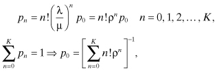
Let pn be the limiting state probability that the process is in state n, n = 0, 1, 2, … . Then applying the balance equations we obtain:
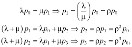
where ρ = λ/μ. Similarly, it can be shown that:
![]()
Since:

we obtain
![]()
Since ρ = 1 – p0, which is the probability that the system is not empty and hence the server is not idle, we call ρ the server utilization (or utilization factor).
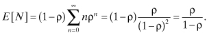
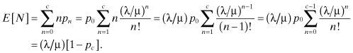
The expected number of customers in the system is given by:

But:

Thus,

Therefore,
We can obtain the mean time in the system from Little’s formula as follows:

where the last result follows from the fact that the mean service time is E[X] = 1/µ. Similarly, the mean waiting time and mean number of customers in queue are given by:

Recall that the mean number of customers in service is E[Ns]. Using the above results we obtain:
![]()
Thus, the mean number of customers in service is ρ, the probability that the server is busy.
Note that the mean waiting time, the mean time in the system, the mean number of customers in the system, and the mean number of customers in queue become extremely large as the server utilization ρ approaches 1. Figure 3.4 illustrates this for the case of the expected waiting time.
Example 3.1:
Students arrive at the campus post office according to a Poisson process with an average rate of one student every 4 min. The time required to serve each student is exponentially distributed with a mean of 3 min. There is only one postal worker at the counter and any arriving student who finds the worker busy joins a queue that is served in an FCFS manner.
a. What is the probability that an arriving student has to wait?
b. What is the mean waiting time of an arbitrary student?
c. What is the mean number of waiting students at the post office?
Solution:
The above problem is an M/M/1 queue with the following parameters:

a. P[arriving student waits] = P[server is busy] = ρ = 0.75
b. E[W] = ρE[X]/(1 – ρ) = (0.75)(3)/(1 – 0.75) = 9 min
c. E[Nq] = λE[W] = (1/4)(9) = 2.25 students.
Example 3.2:
Customers arrive at a checkout counter in a grocery store according to a Poisson process with an average rate of 10 customers per hour. There is only one clerk at the counter and the time to serve each customer is exponentially distributed with a mean of 4 min.
a. What is the probability that a queue forms at the counter?
b. What is the average time a customer spends at the counter?
c. What is the average queue length at the counter?
Solution:
This is an M/M/1 queueing system. We must first convert the arrival and service rates to the same unit of customers per minute since service time is in minutes. Thus, the parameters of the system are as follows:

a. P[queue forms] = P[server is busy] = ρ = 2/3
b. Average time at the counter = E[T] = E[X]/(1 – ρ) = 4/(1/3) = 12 min
c. Average queue length = E[Nq] = ρ2/(1 – ρ) = (4/9)/(1/3) = 4/3 customers
Figure 3.4 Mean waiting time versus server utilization.

3.5.1 Stochastic Balance
A shortcut method of obtaining the steady-state equations in an M/M/1 queueing system is by means of a flow balance procedure called local balance. The idea behind stochastic balance is that in any steady-state condition, the rate at which the process moves from left to right across a “probabilistic wall” is equal to the rate at which it moves from right to left across that wall. For example, Figure 3.5 shows three states n – 1, n, and n + 1 in the state transition rate diagram of an M/M/1 queue.
Figure 3.5 Local balance concept.

The rate at which the process crosses wall A from left to right is λpn–1, which is true because this can only happen when the process is in state n – 1. Similarly, the rate at which the process crosses wall A from right to left is μpn. By stochastic balance we mean that λpn–1 = μpn or pn = (λ/μ)pn–1 = ρpn–1, which is the result we obtained earlier in the analysis of the system.
3.5.2 Total Time and Waiting Time Distributions of the M/M/1 Queueing System
Consider a tagged customer, say customer k, who arrives at the system and finds it in state n. If n > 0, then because of the fact that the service time X is exponentially distributed, the service time of the customer receiving service when the tagged customer arrives “starts from scratch.” Thus, the total time that the tagged customer spends in the system is given by:
![]()
Since the Xk are identically distributed, the s-transform of the probability density function (PDF) of Tk is given by:
![]()
Thus, the unconditional total time in the system is given by:

Since MX(s) = μ/(s + μ), we obtain the following result:
![]()
This shows that T is an exponentially distributed random variable with mean 1/µ(1 – ρ), which agrees with the value of E[T] that we obtained earlier. Similarly, the waiting time distribution can be obtained by considering the experience of the tagged customer in the system, as follows:
![]()
Thus, the s-transform of the PDF of Wk, given that there are n customers when the tagged customer arrives, is given by:

Therefore,

Thus, the PDF and cumulative distribution function (CDF) of W are given by:

where δ(w) is the impulse function. Observe that the mean waiting time is given by:
![]()
which was the result we obtained earlier.
3.6 EXAMPLES OF OTHER M/M QUEUEING SYSTEMS
The goal of this section is to describe some relatives of the M/M/1 queueing systems without rigorously analyzing them as we did for the M/M/1 queueing system. These systems can be used to model different human behaviors and they include:
a. Blocking from entering a queue, which is caused by the fact that the system has a finite capacity and a customer arrives when the system is full.
b. Defections from a queue, which can be caused by the fact that a customer has spent too much time in queue and leaves without receiving service out of frustration. Defection is also called reneging in queueing theory.
c. Jockeying for position among many queues, which can arise when in a multiserver system, each server has its own queue and some customer in one queue notices that another queue is being served faster than his own, thus he leaves his queue and moves into the supposedly faster queue.
d. Balking before entering a queue, which can arise if the customer perceives the queue to be too long and chooses not to join it at all
e. Bribing for queue position, which is a form of dynamic priority because a customer pays some “bribe” to improve his position in the queue. Usually the more bribes he pays, the better position he gets.
f. Cheating for queue position, which is different from bribing because in cheating, the customer uses trickery rather than his personal resources to improve his position in the queue
g. Bulk service, which can be used to model table assignments in restaurants. For example, a queue at a restaurant may appear to be too long, but in actual fact when a table is available (i.e., a server is ready for the next customer), it can be assigned to a family of four, which is identical to serving the four people in queue together.
h. Batch arrival, which can be used to model how friends arrive in groups at a movie theater, concert show or a ball game, or how families arrive at a restaurant. Thus, the number of customers in each arriving batch can be modeled by some probabilistic law.
From this list, it can be seen that queueing theory is a very powerful modeling tool that can be applied to all human activities and hence all walks of life. In the following sections we describe some of the different queueing models that are based on Poisson arrivals and exponentially distributed service times.
3.6.1 The M/M/c Queue: The c-Server System
In this scheme there are c identical servers. When a customer arrives he is randomly assigned to one of the idle servers until all servers are busy when a single queue is formed. Note that if a queue is allowed to form in front of each server, then we have an M/M/1 queue with modified arrival since customers join a server’s queue in some probabilistic manner. In the single queue case, we assume that there is an infinite capacity and service is based on FCFS policy.
The service rate in the system is dependent on the number of busy servers. If only one server is busy, the service rate is μ; if two servers are busy, the service rate is 2µ; and so on until all servers are busy when the service rate becomes cμ. Thus, until all servers are busy the system behaves like a heterogeneous queueing system in which the service rate in each state is different. When all servers are busy, it behaves like a homogeneous queueing system in which the service rate is the same in each state. The state transition rate diagram of the system is shown in Figure 3.6.
Figure 3.6 State transition rate diagram for M/M/c queue.

The service rate is:
![]()
If we define ρ = λ/cμ, then using stochastic balance equations it can be shown that the limiting state probability of being in state n is given by:
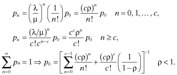
Note that queues can only form when the process is in state c or any state higher than c. Thus, arriving customers who see the system in any state less than c do not have to wait. The probability that a queue is formed is given by:

The expected number of customers in queue is given by:

From Little’s formula, the mean waiting time is given by:
![]()
Finally, the expected time in the system and the expected number of customers in the system are given, respectively, by:

Example 3.3:
Students arrive at a checkout counter in the college cafeteria according to a Poisson process with an average rate of 15 students per hour. There are two cashiers at the counter and they provide identical service to students. The time to serve a student by either cashier is exponentially distributed with a mean of 3 min. Students who find both cashiers busy on their arrival join a single queue. What is the probability that an arriving student does not have to wait?
Solution:
This is an M/M/2 queueing problem with the following parameters with λ and μ in students per minute:

An arriving student does not have to wait if he finds the system either empty or with only one server busy. The probability of this event is p0 + p1 = 35/44.
3.6.2 The M/M/1/K Queue: The Single-Server Finite-Capacity System
In this system, arriving customers who see the system in state K are lost. The state transition rate diagram is shown in Figure 3.7.
Figure 3.7 State transition rate diagram for M/M/1/K queue.

Using the stochastic balance equations, it can be shown that the steady-state probability that the process is in state n is given by:
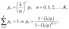
where λ < μ. It can also be shown that the mean number of customers in the system is given by:

Note that all the traffic reaching the system does not enter the system because customers are not allowed into the system when there are already K customers in the system. That is, if we define ρ = λ/μ, then customers are turned away with probability:

Thus, we define the actual rate at which customers arrive into the system, λa, as:
![]()
We can then apply Little’s formula to obtain
![]()
Example 3.4:
Each morning, people arrive at Ed’s garage to fix their cars. Ed’s garage can only accommodate four cars. Anyone arriving when there are already four cars in the garage has to go away without leaving his car for Ed to fix. If Ed’s customers arrive according to a Poisson process with a rate of one customer per hour and the time it takes Ed to service a car is exponentially distributed with a mean of 45 min, what is the probability that an arriving customer finds Ed idle? What is the probability that an arriving customer leaves without getting his car fixed?
Solution:
This is an M/M/1/4 queue with the following parameters:

a. The probability that an arriving customer finds Ed idle is p0 = 0.3278.
b.
The probability that a customer leaves without fixing his car is the probability that he finds the garage full when he arrived, which is ![]() .
.
3.6.3 The M/M/c/c Queue: The c-Server Loss System
This is a very useful model in telephony. It is used to model calls arriving at a telephone switchboard, which usually has a finite capacity. It is assumed that the switchboard can support a maximum of c simultaneous calls (i.e., it has a total of c channels available). Any call that arrives when all c channels are busy will be lost. This is usually referred to as the blocked-calls-lost model. The state transition rate diagram is shown in Figure 3.8.
Figure 3.8 State transition rate diagram for M/M/c/c queue.

Using the stochastic balance equations, it can be shown that the steady-state probability that the process is in state n is given by:

The probability that the process is in state c, pc, is called the Erlang’s loss formula, which is given by:

where ρ = λ/cμ is the utilization factor of the system.
As in the M/M/1/K queueing system, not all traffic enters the system. The actual average arrival rate into the system is:
![]()
Since no customer is allowed to wait, E[W] and E[Nq] are both zero. However, the mean number of customers in the system is:
By Little’s formula,
![]()
This confirms that the mean time a customer admitted into the system spends in the system is the mean service time.
Example 3.5:
Bob established a dial-up service for Internet access. As a small businessman, Bob can only support four channels for his customers. Any of Bob’s customers who want access to the Internet when all four channels are busy are blocked and will have to hang up. Bob’s studies indicate that customers arrive for Internet access according to a Poisson process with an average rate of eight calls per hour and the duration of each call is exponentially distributed with a mean of 10 min. If Jay is one of Bob’s customers, what is the probability that on this particular dial-up attempt he cannot gain access to the Internet?
Solution:
This is an example of M/M/4/4 queueing system. The parameters of the model are as follows:

The probability that Jay is blocked is the probability that he dials up when the process is in state 4. This is given by:

3.6.4 The M/M/1//K Queue: The Single Server Finite Customer Population System
In the previous examples we assumed that the customers are drawn from an infinite population because the arrival process has a Poisson distribution. Assume that there are K potential customers in the population. An example is where we have a total of K machines that can be either operational or down, needing a serviceman to fix them. If we assume that the customers act independently of each other and that given that a customer has not yet come to the service facility, the time until he comes to the facility is exponentially distributed with mean 1/λ, then the number of arrivals when n customers are already in the service facility is governed by a heterogeneous Poisson process with mean λ(K – n). When n = K, there is no more customer left to draw from, which means that the arrival rate becomes zero. Thus, the state transition rate diagram is as shown in Figure 3.9.
Figure 3.9 State transition rate diagram for M/M/1//K queue.

The arrival rate when the process is in state n is:
![]()
Using the stochastic balance equations, it can be shown that the steady-state probabilities are given by:
where ρ = λ/μ. Other finite-population schemes can easily be derived from the above models. For example, we can obtain the state transition rate diagram for the c-server finite population system with population K > c by combining the arriving process on the M/M/1//K queueing system with the service process of the M/M/c queueing system.
Example 3.6:
A small organization has three old PCs, each of which can be working (or operational) or down. When any PC is working, the time until it fails is exponentially distributed with a mean of 10 h. When a PC fails, the repairman immediately commences servicing it to bring it back to the operational state. The time to service each failed PC is exponentially distributed with a mean of 2 h. If there is only one repairman in the facility and the PCs fail independently, what is the probability that the organization has only two PCs working?
Solution:
This is an M/M/1//3 queueing problem in which the arrivals are PCs that have failed and the single server is the repairman. Thus, when the process is in state 0 all PCs are working; when it is in state 1, two PCs are working; when it is in state 2, only one PC is working; and when it is in state 3, all PCs are down, awaiting repair. The parameters of the problem are:

As stated earlier, the probability that two computers are working is the probability that the process is in state 1, which is given by:
![]()
3.7 M/G/1 QUEUE
In this system, customers arrive according to a Poisson process with rate λ and are served by a single server with a general service time X whose PDF is fX(x), x ≥ 0, mean is E[X], second moment is E[X2], and variance is ![]() . The capacity of the system is infinite and customers are served on an FCFS basis. Thus, the service time distribution does not have the memoryless property of the exponential distribution, and the number of customers in the system time t, N(t), is not a Poisson process. A more appropriate description of the state at time t includes both N(t) and the residual life of the service time of the current customer. That is, if R denotes the residual life of the current service, then the set of pairs {(N, R)} provides the description of the state space. Thus, we have a two-dimensional state space, which is a somewhat complex way to proceed with the analysis. However, the analysis is simplified if we can identify those points in time where the state is easier to describe. Such points are usually chosen to be those time instants at which customers leave the system, which means that R = 0.
. The capacity of the system is infinite and customers are served on an FCFS basis. Thus, the service time distribution does not have the memoryless property of the exponential distribution, and the number of customers in the system time t, N(t), is not a Poisson process. A more appropriate description of the state at time t includes both N(t) and the residual life of the service time of the current customer. That is, if R denotes the residual life of the current service, then the set of pairs {(N, R)} provides the description of the state space. Thus, we have a two-dimensional state space, which is a somewhat complex way to proceed with the analysis. However, the analysis is simplified if we can identify those points in time where the state is easier to describe. Such points are usually chosen to be those time instants at which customers leave the system, which means that R = 0.
To obtain the steady-state analysis of the system, we proceed as follows. Consider the instant the kth customer arrives at the system. Assume that the ith customer was receiving service when the kth customer arrived. Let Ri denote the residual life of the service time of the ith customer at the instant the kth customer arrived, as shown in Figure 3.10.
Figure 3.10 Service experience of the ith customer in M/G/1 queue.

Assume that Nqk customers were waiting when the kth customer arrived. Since the service times are identically distributed, the waiting time Wk of the kth customer is given by:
![]()
where u(k) is an indicator function that has a value of 1 if the server was busy when the kth customer arrived and zero otherwise. That is, if Nk defines the total number of customers in the system when the kth customer arrived, then:
![]()
Thus, taking expectations on both sides and noting that Nqk and X are independent random variables, and also that u(k) and Ri are independent random variables, we obtain:
![]()
Now, from the principles of random incidence in a renewal process, we know that:
![]()
Also,
![]()
Finally, from Little’s formula, E[Nqk] = λE[Wk]. Thus, the mean waiting time of the kth customer is given by:

Since the experience of the kth customer is a typical experience, we conclude that the mean waiting time in an M/G/1 queue is given by:
![]()
Thus, the expected number of customers in the system is given by:
![]()
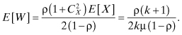
This expression is called the Pollaczek–Khinchin formula. It is sometimes written in terms of the coefficient of variation CX of the service time. The square of CX is defined as follows:

Thus, the second moment of the service time becomes ![]() , and the Pollaczek–Khinchin formula becomes:
, and the Pollaczek–Khinchin formula becomes:

Similarly, the mean waiting time becomes:

3.7.1 Waiting Time Distribution of the M/G/1 Queue
We can obtain the distribution of the waiting time as follows. Let Nk denote the number of customers left behind by the kth departing customer, and let Ak denote the number of customers that arrive during the service time of the kth customer. Then we obtain the following relationship:
![]()
Thus, we see that ![]() forms a Markov chain called the imbedded M/G/1
Markov chain. Let the transition probabilities of the imbedded Markov chain be defined as follows:
forms a Markov chain called the imbedded M/G/1
Markov chain. Let the transition probabilities of the imbedded Markov chain be defined as follows:
![]()
Since Nk cannot be greater than Nk + 1 + 1 we have that pij = 0 for all j < i – 1. For j ≥ i – 1, pij is the probability that exactly j – i + 1 customers arrived during the service time of the (k + 1)th customer, i > 0. Also, since the kth customer left the system empty in state 0, p0j represents the probability that exactly j customers arrived while the (k + 1)th customer was being served. Similarly, since the kth customer left one customer behind, which is the (k + 1)th customer, in state 1, p1j is the probability that exactly j customers arrived while the (k + 1)th customer was being served. Thus, p0j = p1j for all j. Let the random variable AS denote the number of customers that arrive during a service time. Then the probability mass function (PMF) of AS is given by:
![]()
If we define αn = P[AS = n], then the state transition matrix of the imbedded Markov chain is given as follows:

The state transition diagram is shown in Figure 3.11.
Figure 3.11 Partial state transition diagram for M/G/1 imbedded Markov chain.

Observe that the z-transform of the PMF of AS is given by:

where MX(s) is the s-transform of the PDF of X, the service time. That is, the z-transform of the PMF of AS is equal to the s-transform of the PDF of X evaluated at the point s = λ – λz. Let fT(t) denote the PDF of T, the total time in the system. Let K be a random variable that denotes the number of customers that a tagged customer leaves behind. This is the number of customers that arrived during the total time that the tagged customer was in the system. Thus, the PMF of K is given by:
![]()
As in the case of AS, it is easy to show that the z-transform of the PMF of K is given by:
![]()
Recall that Nk, the number of customers left behind by the kth departing customer, satisfies the relationship:
![]()
where Ak denotes the customers that arrive during the service time of the kth customer. Thus, K is essentially the value of Nk for our tagged customer. It can be shown that the z-transform of the PMF of K is given by:
![]()
Thus, we have that:
![]()
If we set s = λ – λz, we obtain the following:
![]()
This is one of the equations usually called the Pollaczek–Khinchin formula. Finally, since T = W + X, which is the sum of two independent random variables, we have that the s-transform of T is given by:
![]()
From this we obtain the s-transform of the PDF of W as:
![]()
This is also called the Pollaczek–Khinchin formula. The expected value is given by:
![]()
which agrees with the earlier result. Note that the derivation of the previous result was based on an arriving customer’s viewpoint while the current result is based on a departing customer’s viewpoint. We are able to obtain the same mean waiting for both because the arrival process is a Poisson process. The Poisson process possesses the so-called PASTA property (Wolff 1982, 1989). PASTA is an acronym for “Poisson arrivals see time averages,” which means that customers with Poisson arrivals see the system as if they came into it at a random instant despite the fact that they induce the evolution of the system. Assume that the process is in equilibrium. Let πk denote the probability that the system is in state k at a random instant, and let ![]() denote the probability that the system is in state k just before a random arrival occurs. Generally,
denote the probability that the system is in state k just before a random arrival occurs. Generally, ![]() ; however, for a Poisson process,
; however, for a Poisson process, ![]() .
.
3.7.2 The M/Ek/1 Queue
The M/Ek/1 queue is an M/G/1 queue in which the service time has the Erlang-k distribution. It is usually modeled by a process in which service consists of a customer passing, stage by stage, through a series of k independent and identically distributed subservice centers, each of which has an exponentially distributed service time with mean 1/kµ. Thus, the total mean service time is k × (1/kµ) = 1/µ. The state transition rate diagram for the system is shown in Figure 3.12. Note that the states represent service stages. Thus, when the system is in state 0, an arrival causes it to go to state k; when the system is in state 1, an arrival causes it to enter state k + 1, and so on. A completion of service at state j leads to a transition to state j – 1, j ≥ 1.
Figure 3.12 State transition rate diagram for the M/Ek/1 queue.

While we can analyze the system from scratch, we can also apply the results obtained for the M/G/1 queue. We know for an Erlang-k random variable X, the following results can be obtained:

Thus, we obtain the following results:
a. The mean waiting time is:
b. The s-transform of the PDF of the waiting time is:

c. The mean total number of customers in the system is:

d. The s-transform of the PDF of the total time in the system is:

3.7.3 The M/D/1 Queue
The M/D/1 queue is an M/G/1 queue with a deterministic (or fixed) service time. We can analyze the queueing system by applying the results for M/G/1 queueing system as follows:

Thus, we obtain the following results:
a. The mean waiting time is:

b. The s-transform of the PDF of the waiting time is:
![]()
c. The mean total number of customers in the system is:

d. The s-transform of the PDF of the total time in the system is:
![]()
3.7.4 The M/M/1 Queue
The M/M/1 queue is also an example of the M/G/1 queue with the following parameters:

When we substitute for these parameters in the equations for M/G/1, we obtain the results previously obtained for M/M/1 queueing system.
3.7.5 The M/Hk/1 Queue
This is a single-server, infinite-capacity queueing system with Poisson arrivals and hyperexponentially distributed service time of order k. That is, with probability θj, an arriving customer will choose to receive service from server j whose service time is exponentially distributed with a mean of 1/µj, 1 ≤ j ≤ k, where:

The system is illustrated in Figure 3.13.
Figure 3.13 A k-stage hyperexponential server.

For this system we have that:

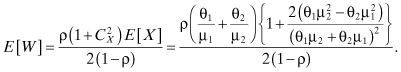
For the special case of k = 2, that is, for the M/H2/1 queue, we have the following results:

From this we obtain the following performance parameters:
a. The mean waiting time is:
b. The s-transform of the PDF of the waiting time is:
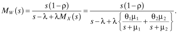
c. The mean total number of customers in the system is:

d. The s-transform of the PDF of the total time in the system is:

3.8 PROBLEMS
3.1 People arrive to buy tickets at a movie theater according to a Poisson process with an average rate of 12 customers per hour. The time it takes to complete the sale of a ticket to each person is exponentially distributed with a mean of 3 min. There is only one cashier at the ticket window, and any arriving customer who finds the cashier busy joins a queue that is served in an FCFS manner.
a. What is the probability that an arriving customer does not have to wait?
b. What is the mean number of waiting customers at the window?
c. What is the mean waiting time of an arbitrary customer?
3.2 Cars arrive at a car wash according to a Poisson process with a mean rate of eight cars per hour. The policy at the car wash is that the next car cannot pass through the wash procedure until the car in front of it is completely finished. The car wash has a capacity to hold 10 cars, including the car being washed, and the time it takes a car to go through the wash process is exponentially distributed with a mean of 6 min. What is the average number of cars lost to the car wash company every 10-h day as a result of the capacity limitation?
3.3 A shop has five identical machines that break down independently of each other. The time until a machine breaks down is exponentially distributed with a mean of 10 h. There are two repairmen who fix the machines when they fail. The time to fix a machine when it fails is exponentially distributed with a mean of 3 h, and a failed machine can be repaired by either of the two repairmen. What is the probability that exactly one machine is operational at any one time?
3.4 People arrive at a phone booth according to a Poisson process with a mean rate of five people per hour. The duration of calls made at the phone booth is exponentially distributed with a mean of 4 min.
a. What is the probability that a person arriving at the phone booth will have to wait?
b. The phone company plans to install a second phone at the booth when it is convinced that an arriving customer would expect to wait at least 3 min before using the phone. At what arrival rate will this occur?
3.5 People arrive at a library to borrow books according to a Poisson process with a mean rate of 15 people per hour. There are two attendants at the library, and the time to serve each person by either attendant is exponentially distributed with a mean of 3 min.
a. What is the probability that an arriving person will have to wait?
b. What is the probability that one or both attendants are idle?
3.6 A company is considering how much capacity K to provide in its new service facility. When the facility is completed, customers are expected to arrive at the facility according to a Poisson process with a mean rate of 10 customers per hour, and customers who arrive when the facility is full are lost. The company hopes to hire an attendant to serve at the facility. Because the attendant is to be paid by the hour, the company hopes to get its money’s worth by making sure that the attendant is not idle for more than 20% of the time he or she should be working. The service time is expected to be exponentially distributed with a mean of 5.5 min.
a. How much capacity should the facility have to achieve this goal?
b. With the capacity obtained in part a, what is the probability that an arriving customer is lost?
3.7 A small private branch exchange (PBX) serving a startup company can only support five lines for communication with the outside world. Thus, any employee who wants to place an outside call when all five lines are busy is blocked and will have to hang up. A blocked call is considered to be lost because the employee will not make that call again. Calls to the outside world arrive at the PBX according to a Poisson process with an average rate of six calls per hour, and the duration of each call is exponentially distributed with a mean of 4 min.
a. What is the probability that an arriving call is blocked?
b. What is the actual arrival rate of calls to the PBX?
3.8 A cybercafé has six PCs that customers can use for Internet access. These customers arrive according to a Poisson process with an average rate of six per hour. Customers who arrive when all six PCs are being used are blocked and have to go elsewhere for their Internet access. The time that a customer spends using a PC is exponentially distributed with a mean of 8 min.
a. What fraction of arriving customers are blocked?
b. What is the actual arrival rate of customers at the cafe?
c. What fraction of arriving customers would be blocked if one of the PCs is out of service for a very long time?
3.9 Consider a birth and death process representing a multiserver finite population system with the following birth and death rates:
![]()
a. Find the pk, k = 0, 1, 2, 3, 4 in terms of λ and μ.
b. Find the average number of customers in the system.
3.10 Students arrive at a checkout counter in the college cafeteria according to a Poisson process with an average rate of 15 students per hour. There are three cashiers at the counter, and they provide identical service to students. The time to serve a student by any cashier is exponentially distributed with a mean of 3 min. Students who find all cashiers busy on their arrival join a single queue. What is the probability that at least one cashier is idle?
3.11 Customers arrive at a checkout counter in a grocery store according to a Poisson process with an average rate of 10 customers per hour. There are two clerks at the counter and the time either clerk takes to serve each customer is exponentially distributed with an unspecified mean. If it is desired that the probability that both cashiers are idle is to be no more than 0.4, what will be the mean service time?
3.12 Consider an M/M/1/5 queueing system with mean arrival rate λ and mean service time 1/µ that operates in the following manner. When any customer is in queue, the time until he defects (i.e., leaves the queue without receiving service) is exponentially distributed with a mean of 1/β. It is assumed that when a customer begins receiving service he does not defect.
a. Give the state transition rate diagram of the process.
b. What is the probability that the server is idle?
c. Find the average number of customers in the system.
3.13 Consider an M/M/1 queueing system with mean arrival rate λ and mean service time 1/µ that operates in the following manner. When the number of customers in the system is greater than three, a newly arriving customer joins the queue with probability p and balks (i.e., leaves without joining the queue) with probability 1 – p.
a. Give the state transition rate diagram of the process.
b. What is the probability that the server is idle?
c. Find the actual arrival rate of customers in the system.
3.14 Consider an M/M/1 queueing system with mean arrival rate λ and mean service time 1/µ. The system provides bulk service in the following manner. When the server completes any service, the system returns to the empty state if there are no waiting customers. Customers who arrive while the server is busy join a single queue. At the end of a service completion, all waiting customers enter the service area to begin receiving service.
a. Give the state transition rate diagram of the process.
b. What is the probability that the server is idle?
3.15 Consider an M/G/1 queueing system where service is rendered in the following manner. Before a customer is served, a biased coin whose probability of heads is p is flipped. If it comes up heads, the service time is exponentially distributed with mean 1/µ1. If it comes up tails, the service time is constant at d. Calculate the following:
a. The mean service time, E[X]
b. The coefficient of variation, CX, of the service time
c. The expected waiting time, E[W]
d. The s-transform of the PDF of W
3.16 Consider a queueing system in which customers arrive according to a Poisson process with rate λ. The time to serve a customer is a third-order Erlang random variable with parameter μ. What is the expected waiting time of a customer?