
“It is white.” | ||
| --George W. Bush, after being asked by a child in Britain what the White House was like, July 19, 2001 | ||
In this chapter, we introduce the notion of in-memory fuzzing, a novel approach to fuzzing that has received little public attention and for which no full-featured proof of concept tools have yet been publicly released. In essence, this technique aims to transition fuzzing from the familiar client–server (or client–target) model, to a target-only model residing solely in memory. Although technically this is a more complex approach that requires strong low-level knowledge of assembly language, process memory layout, and process instrumentation, there are a number of benefits to the technique that we outline prior to jumping into any specific implementation details.
In previous chapters, we made a concerted effort to provide an unbiased view from both the UNIX and Windows perspective. Due to the complex scope of this fuzzing technique, we limit our focus in this chapter to a single platform. We chose Microsoft Windows as the platform of focus for a number of reasons. First, this fuzzing technique is better applied against closed source targets, as binary software distributions are more popular on the Windows platform than on UNIX. Second, Windows exposes rich and powerful debugging APIs for process instrumentation. That is not to say that debugging APIs are unavailable on UNIX platforms, but we are of the opinion that they are simply not as robust. The general ideas and approaches discussed here can, of course, be adopted to apply across various platforms.
Every method of fuzzing we’ve discussed so far has required the generation and transmission of data over expected channels. In Chapter 11, “File Format Fuzzing,” Chapter 12, “File Format Fuzzing: Automation on UNIX,” and Chapter 13, “File Format Fuzzing: Automation on Windows,” mutated files were loaded directly by the application. In Chapter 14, “Network Protocol Fuzzing,” Chapter 15, “Network Protocol Fuzzing: Automation on UNIX,” and Chapter 16, “Network Protocol Fuzzing: Automation on Windows,” fuzz data was transmitted over network sockets to target services. Both situations require that we represent a whole file or a complete protocol to the target, even if we are interested only in fuzzing a specific field. Also in both situations, we were largely unaware and indifferent to what underlying code was executed in response to our inputs.
In-memory fuzzing is an altogether different animal. Instead of focusing on a specific protocol or file format, we focus instead on the actual underlying code. We are shifting our focus from data inputs to the functions and individual assembly instructions responsible for parsing data inputs. In this manner we skip the expected data communications channel and instead focus on either mutating or generating data within the memory of the target application.
When is this beneficial? Consider the situation where you are fuzzing a closed source network daemon that implements a complex packet encryption or obfuscation scheme. To successfully fuzz this target it is first necessary to completely reverse engineer and reproduce the obfuscation scheme. This is a prime candidate for in-memory fuzzing. Instead of focusing unnecessarily on the protocol encapsulation, we peer into the memory space of the target application looking for interesting points, for example, after the received network data has been deobfuscated. As another example, consider the situation where we wish to test the robustness of a specific function. Say that through some reverse engineering efforts we have pinned down an e-mail parsing routine that takes a single string argument, an e-mail address, and parses it in some fashion. We could generate and transmit network packets or test files containing mutated e-mail addresses, but with in-memory fuzzing we can focus our efforts by directly fuzzing the target routine.
These concepts are further clarified throughout the remainder of this chapter as well as the next one. First, however, we need to cover some background information.
Before we continue any further, let’s run through a crash course of the Microsoft Windows memory model, briefly discussing the general layout and properties of the memory space of a typical Windows process. We’ll touch on a number of complex and detailed subject matter areas in this section that we encourage you to delve into further. As some of this material tends to be quite dry, feel free to skip through to the overview and proceed directly to the diagram at the end if you so choose.
Since Windows 95, the Windows operating system has been built on the flat memory model, which on a 32-bit platform provides a total of 4GB of addressable memory. The 4GB address range, by default, is divided in half. The bottom half (0x00000000–0x7FFFFFFF) is reserved for user space and the top half (0x80000000–0xFFFFFFFF) is reserved for kernel space. This split can be optionally changed to 3:1 (through the /3GB boot.ini setting [1]), 3GB for user space and 1GB for the kernel, for improved performance in memory-intensive applications such as Oracle’s database. The flat memory model, as opposed to the segmented memory model, commonly uses a single memory segment for referencing program code and data. The segmented memory model, on the other hand, utilizes multiple segments for referencing various memory locations. The main advantages of the flat memory model versus the segmented memory model are drastic performance gains and decreased complexity from the programmer’s viewpoint as there is no need for segment selection and switching. Even further simplifying the world for programmers, the Windows operating system manages memory via virtual addressing. In essence, the virtual memory model presents each running process with its own 4GB virtual address space. This task is accomplished through a virtual-to-physical address translation aided by a memory management unit (MMU). Obviously, not very many systems can physically support providing 4GB of memory to every running process. Instead, virtual memory space is built on the concept of paging. A page is a contiguous block of memory with a typical size of 4,096 (0x1000) bytes in Windows. Pages of virtual memory that are currently in use are stored in RAM (primary storage). Unused pages of memory can be swapped to disk (secondary storage) and later restored to RAM when needed again.
Another important concept in Windows memory management is that of memory protections. Memory protection attributes are applied at the finest granularity on memory pages; it is not possible to assign protection attributes to only a portion of page. Some of the available protection attributes that might concern us include:[2]
PAGE_EXECUTE. Memory page is executable, attempts to read from or write to the page results in an access violation.
PAGE_EXECUTE_READ. Memory page is executable and readable, attempts to write to the page result in an access violation.
PAGE_EXECUTE_READWRITE. Memory page is fully accessible. It is executable, can be read from and written to.
PAGE_NOACCESS. Memory page is not accessible. Any attempt to execute from, read from, or write to the memory page results in an access violation.
PAGE_READONLY. Memory page is readable only. Any attempt to write to the memory page results in an access violation. If the underlying architecture supports differentiating between reading and executing (not always the case), then any attempt to execute from the memory page also results in an access violation.
PAGE_READWRITE. Memory page is readable and writable. As with PAGE_READONLY, if the underlying architecture supports differentiating between reading and executing, then any attempt to execute from the memory page results in an access violation.
For our purposes we might only be interested in the PAGE_GUARD modifier, which according to MSDN [3] raises a STATUS_GUARD_PAGE_VIOLATION on any attempt to access the guarded page and then subsequently removes the guard protection. Essentially, PAGE_GUARD acts as a one-time access alarm. This is a feature we might want to use to monitor for access to certain regions of memory. Alternatively we could also use the PAGE_NOACCESS attribute.
Familiarity with memory pages, layout, and protection attributes are important for purposes of in-memory fuzzing, as we will see in the next chapter. Memory management is a complex subject that is heavily discussed in many other publications.[4] We encourage you to reference these other works. For our purposes however all you need to know is the following:
Every Windows process “sees” its own 4GB virtual address space.
Only the bottom 2GB from 0x00000000 through 0x7FFFFFFF are available for user space, the upper 2GB are reserved as kernel space.
The virtual address space of a process is implicitly protected from access by other processes.
The 4GB address space is broken into individual pages with a typical size of 4,096 bytes (0x1000).
At the finest granularity, memory protection attributes are applied to individual memory pages.
The PAGE_GUARD memory protection modifier can be used as a one-time page access alarm.
Study Figure 19.1 to gain a better understanding of where specific elements can be found in the virtual address space of the typical Windows process. Figure 19.1 serves as a useful reference in the next chapter as well, when we discuss the specific development details of an in-memory fuzzing automation tool. Following the figure is a brief description of the various listed elements, in case you are not familiar with them.
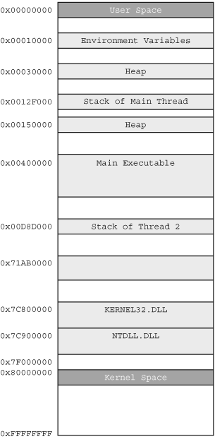
Let’s briefly describe the various elements shown in Figure 19.1 for the benefit of those who are not familiar with them. Starting at the lowest address range, we find the process environment variables at 0x00010000. Recall from Chapter 7, “Environment Variable and Argument Fuzzing,” that environment variables are systemwide global variables that are used to define certain behaviors of applications. Higher up in the address range we find two ranges of memory dedicated to the heap at 0x00030000 and 0x00150000. The heap is a pool of memory from which dynamic memory allocations occur through calls such as malloc() and HeapAlloc(). Note that there can be more then one heap for any given process, just as the diagram shows. Between the two heap ranges we find the stack of the main thread at address 0x0012F000. The stack is a last-in, first-out data structure that is used to keep track of function call chains and local variables. Note that each thread within a process has its own stack. In our example diagram, the stack of thread 2 is located at 0x00D8D000. At address 0x00400000 we find the memory region for our main executable, the .exe file that we executed to get the process loaded in memory. Toward the upper end of the user address space we find a few system DLLs, kernel32.dll and ntdll.dll. DLLs are Microsoft’s implementation of shared libraries, common code that is used across applications and exported through a single file. Executables and DLLs both utilize the Portable Executable (PE) file format. Note that the addresses shown in Figure 19.1 will not be the same from process to process and were chosen here simply for example purposes.
Again, we’ve touched on a number of complex subjects that deserve their own books. We encourage you to reference more in-depth materials. However, for our purposes, we should have armed ourselves with enough information to dive into the subject at hand.
We outline and implement two approaches to in-memory fuzzing in this book. In both cases, we are moving our fuzzer from outside the target to within the target itself. The process is best explained and understood visually. To begin, consider Figure 19.2, which depicts a simple control flow diagram of a fictitious but typical networked target.
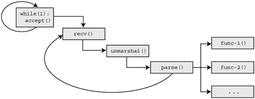
A loop within the main thread of our example target application is awaiting new client connections. On receiving a connection, a new thread is spawned to process the client request, which is received through one or more calls to recv(). The collected data is then passed through some form of unmarshaling or processing routine. The unmarshal() routine might be responsible for protocol decompression or decryption but does not actually parse individual fields within the data stream. The processed data is in turn passed to the main parsing routine parse(), which is built on top of a number of other routines and library calls. The parse() routine processes the various individual fields within the data stream, taking the appropriate requested actions before finally looping back to receive further instructions from the client.
Given this situation, what if instead of transmitting our fuzz data across the wire, we could skip the networking steps entirely? Such code isolation allows us to work directly with the routines which we are most likely going to find bugs, such as the parsing routine. We can then inject faults into the routine and monitor the outcome of those changes while drastically increasing the efficiency of the fuzzing process as everything is done within memory. Through the use of some form of process instrumentation we want to “hook” into our target just before the parsing routines, modify the various inputs the routines accept, and let the routines run their course. Obviously as the subject of this book is fuzzing, we of course want the ability to loop through these steps, automatically modifying the inputs with each iteration and monitoring the results.
Arguably the most time-consuming requirement for building a network protocol or file format fuzzer is the dissection of the protocol and file format themselves. There have been attempts at automatic protocol dissection that borrow from the field of bioinformatics, a subject that we touch on in Chapter 22, “Automated Protocol Dissection.” However, for the most part, protocol dissection is a manual and tedious process.
When dealing with the standard documented protocols such as SMTP, POP, and HTTP, for example, you have the benefit of referencing numerous sources such as RFCs, open source clients, and perhaps even previously written fuzzers. Furthermore, considering the widespread use of these protocols by various applications, it might be worthwhile to implement the protocol in your fuzzer, as it will see a lot of reuse. However, you will frequently find yourself in the situation where the target protocol is undocumented, complex, or proprietary. In such cases where protocol dissection might require considerable time and resources, in-memory fuzzing might serve as a viable time-saving alternative.
What if a target communicates over a trivial protocol that is encapsulated within an open encryption standard? Even worse, what if the protocol is encapsulated within a proprietary encryption or obfuscation scheme? The ever so popular Skype[5] communication suite is a perfect example of a difficult target to audit. The EADS/CRC security team went to great lengths[6] to break beyond the layers of obfuscation and uncover a critical Skype security flaw (SKYPE-SB/2005-003).[7] You might be able to sidestep the problem if the target exposes a nonencrypted interface, but what if it does not? Encrypted protocols are one of the major fuzzing show stoppers. In-memory fuzzing might also allow you to avoid the painstaking process of reverse engineering the encryption routine.
You must consider many factors before committing to this approach when fuzzing your target, the first and most significant being that in-memory fuzzing requires reverse engineering of the target to locate the optimal “hook” points, so the cost of entry could be stifling. In general, in-memory fuzzing is best targeted against closed source targets running on a platform supported by your in-memory fuzzing tools.
The first method of in-memory fuzzing we refer to is mutation loop insertion (MLI). MLI requires that we first manually, through reverse engineering, locate the start and end of the parse() routine. Once located, our MLI client can insert a mutate() routine into the memory space of the target. The mutation routine is responsible for transforming the data being handled by the parsing routine and can be implemented in a number of ways that we’ll cover specifically in the next chapter. Next, our MLI client will insert unconditional jumps from the end of the parsing routine to the start of the mutation routine and the end of the mutation routine to the start of the parsing routine. After this is all said and done, the control flow diagram of our target would look like what’s shown in Figure 19.3.
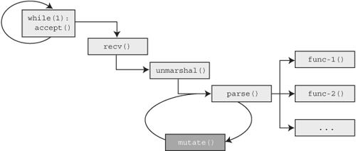
So what happens now? We’ve created a self-sufficient data mutation loop around the parsing code of our target. There’s no longer a need to remotely connect to our target and send data packets. Naturally, this is a significant time saver. Each iteration of the loop will pass different, potentially fault inducing, data to the parsing routines as dictated by mutate().
It goes without saying that our contrived example is overly simplified. Although this was done purposefully to serve as a digestible introduction, it is important to note that in-memory fuzzing is highly experimental. We’ll get into these details in Chapter 20, “In-Memory Fuzzing: Automation,” as we construct a functional fuzzer.
The second method of in-memory fuzzing we refer to as snapshot restoration mutation (SRM). Like MLI, we want to bypass the network-centric portions of our target and attack the focal point, in this case the parse() routine. Also like MLI, SRM requires locating the start and end of the parsing code. With these locations marked, our SRM client will take a snapshot of the target process when the start of the parsing code is reached. Once parsing is complete, our SRM client will restore the process snapshot, mutate the original data, and reexecute the parsing code. The modified control flow diagram of our target will look like what’s shown in Figure 19.4.
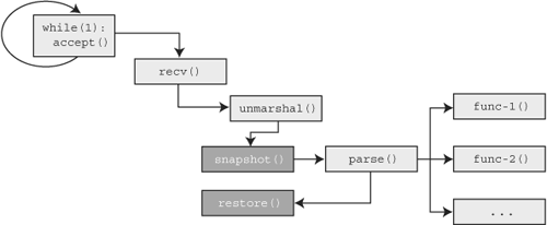
Again, we’ve created a self-sufficient data mutation loop around the parsing code of our target. In Chapter 20, we cover the implementation of a functional proof of concept tool to apply both of these described methods in practice. The prototype-quality fuzzer that we construct will help us empirically determine the specific pros and cons of each approach. First, however, let’s discuss in more detail one of the major benefits of in-memory fuzzing.
There is an unavoidable lag associated with network protocol testing in the traditional client–target model. Test cases must individually be transmitted over the wire and depending on the complexity of the fuzzer, the response from the target must be read back and processed. This lag is further exacerbated when fuzzing deep protocol states. Consider, for example, the POP mail protocol that typically provides service over TCP port 110. A valid exchange to retrieve mail might look like (user inputs highlighted in bold) this:
$ nc mail.example.com 110
+OK Hello there.
user [email protected]
+OK Password required.
pass xxxxxxxxxxxx
+OK logged in.
list
+OK
1 1673
2 19194
3 10187
... [output truncated]...
.
retr 1
+OK 1673 octets follow.
Return-Path: <[email protected]>
Delivered-To: [email protected]
...[output truncated]...
retr AAAAAAAAAAAAAAAAAAAAAAA
-ERR Invalid message number. Exiting.
For our network fuzzer to target the argument of the RETR verb, it will have to step through the required process states by reconnecting and reauthenticating with the mail server for each test case. Instead, we could focus solely on the parsing of the RETR argument by testing only at the desired process depth through one of the previously described in-memory fuzzing methods. Recall that process depth and process state were explained in Chapter 4, “Data Representation and Analysis.”
One of the benefits of in-memory fuzzing is detection of fuzzer-induced faults. Since we are already operating on our target at such a low level, this is an easy addition for the most part. With both the MLI and SRM approaches, our fuzzer, if implemented as a debugger (which it will be), can monitor for exceptional conditions during each mutated iteration. The location of the fault can be saved in conjunction with runtime context information that a researcher can later examine to determine the precise location of the bug. You should note that targets that utilize anti-debugging methodologies, such as Skype previously mentioned, will get in the way of this chosen implementation method.
Our biggest difficulty with fault detection will be filtering out the false positives. Much in the same regard as the Heisenberg uncertainty principle,[8] the sheer act of observing our target process under the microscope of in-memory fuzzing causes it to behave differently. As we are directly modifying the process state of the target in ways that were definitely not originally intended, there is a lot of room for irrelevant faults to occur. Consider Figure 19.5.
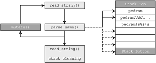
We applied MLI to wrap around parse_name() and read_string(). With each iteration the input to parse_name() is mutated in an attempt to induce fault. However, because we hook after stack allocations are made and just prior to the stack correction, we are continuously losing stack space with each loop iteration. Eventually, we will exhaust the available stack space and thereby cause an unrecoverable fault that was entirely induced by our fuzzing process and not an existing fault within the target.
In-memory fuzzing is not an endeavor for the faint of heart. Before any testing can take place, a skilled researcher must reverse engineer the target to pinpoint the insertion and instrumentation points. Researchers are also required to determine if issues discovered through in-memory fuzzing are indeed accessible with user inputs under normal circumstances. In most cases there will be no such thing as an “immediate” find, but rather a potential input to consider. These setbacks are outweighed by the many benefits provided by the technique.
To our knowledge, the notion of in-memory fuzzing was first introduced to the public by Greg Hoglund of HBGary LLC at the BlackHat Federal[9] and Blackhat USA[10] Security conferences in 2003. HBGary offers a commercial in-memory fuzzing solution called Inspector[11]. In his presentation, Hoglund hints at some of his proprietary technology when mentioning process memory snapshots. Memory snapshots are one of the techniques that we discuss in detail during the creation of an automation tool.
In the next chapter we also step through the implementation and usage of a custom in-memory fuzzing framework. To our knowledge, this is the first open source proof of concept code to tackle the task. As advancements are made to the framework they will be posted on the book’s Web site at http://www.fuzzing.org.
[4] Microsoft Windows Internals, Fourth Edition, Mark E. Russinovich, David A. Solomon; Undocumented Windows 2000 Secrets: A Programmer’s Cookbook, Sven Schreiber; Undocumented Windows NT, Prasad Dabak, Sandeep Phadke, Milind Borate.