
12
Estimation of Nonperforming Assets of Indian Commercial Banks Using Fuzzy AHP and Goal Programming
Kandarp Vidyasagar* and Rajiv Kr. Dwivedi
University Department of Mathematics, Vinoba Bhave University, Hazaribagh, Jharkhand, India
Abstract
The present study computes the various parameters, which are different subdivis ions of the total nonperforming assets (NPA) of Indian Commercial Bank from the financial year 2013–2014 to 2019–2020. The variables were preferred on the several subdivisions. The secondary data have been collected from the audited annual reports of the State Bank of India. Multiple linear equations have been formulated, and Fuzzy Analytic Hierarchy Process (AHP) with extended Saaty’s scale was used for weight estimation of the several parameters. Under these constraints, the goal programming model is developed, and the final result has been obtained using Lingo19. The study reveals that the various subdivisions of both the priority and nonpriority sectors of the Indian economy, which include agriculture and allied activities, industries (macro and small, medium and large), and personal loans have shown a moderate growth in order to increase the total NPA. On the contrary, the drastic growth has been observed in NPA of Services (priority and nonpriority sectors), which has crossed the model results. Further studies were suggested by partitioning the time period on a quarterly basis for the samples and calculating over the various microeconomic and macroeconomic factors and other bank-specific variables for more enhancement.
Keywords: Nonperforming assets, fuzzy AHP, goal programming
12.1 Introduction
Analyzing a diversified set of objectives to obtain the best prediction is cumbersome. Achieving the target level is an out dare without decision making. Over the past few decades, various approaches and mathematical model have been developed to solve the real world problems. Goal programming (GP) is a robust method to solve such problems having multiple objectives. Initially, GP was introduced by Charnes and Cooper (1961) [1]. Later, it became very popular because of its simple method and easy application. GP is a branch of multiobjective optimization, which is a part of multicriteria decision analysis, which helps us in solving multiple conflicting objective measures. The basic aim of GP is to incorporate all goals in a single model that can further be solved simultaneously. The linear programming has a lousy efficacy over goal programming because of its computational efficiency [2].
In 1965, Zadeh propounded the fuzzy set theory [3]. Zimmerman used the membership function of fuzzy sets for the first time in goal programming [4, 5]. An ambient overview on the current study for fuzzy AHP and GP was discussed for optimization of bank liquidity [6]. Integrated method using fuzzy AHP and goal programming was developed for a supplier selection problem [7]. Fuzzy AHP has been used to asses a methodology for water management [8]. Fuzzy AHP and DEMATEL-ANP were combined to make a new hybrid multicriteria decision making model for selecting best space for free time in an urban site [9]. Weighted linear model for Fuzzy Goal Programming was developed, which could easily be used to solve real life problems [10]. Several researchers developed models for real time decision problem using fuzzy goal programming, such as vendor selection in supply chain, has been solved using the same approach [11]. Further, Fuzzy AHP and Fuzzy Goal Programming were together used for solving six primary goals in project selection, such as maximization of profit, customer satisfaction, processing capability along with minimization of cost, completion time, and risk [12].
Nonperforming assets (NPAs) are those credit facility in which the interest and instalment of principal remained due for a defined time period. NPA has been classified as substandard doubtful and loss category on the basis of various criteria speculated by Reverse Bank of India (RBI). A loan amount is considered as substandard assets if it remains nonperforming for a period less than or up to 1 year. Doubtful assets are those assets, which remained under substandard category for 1 year. Loss assets are those in which loss has been identified, but has not been fully written off. NPAs of Scheduled commercial banks (SCBs) increased from Rs 3, 23, 464 crore as on March 31, 2016 to Rs10, 6, 187 crore as on March 31, 2018. The main reason behind this drastic increase in NPAs was demonetization [13]. After 2018, there was a downfall in NPAs by Rs 1, 02, 562 crore and new figure in March 31, 2019, was Rs. 9, 33, 625 crore. The parlous state of NPA in Indian bank was already a matter of severe concern before COVID-19 struck.
The prolonged lockdown all over the country has certainly downturn the economic parameter and disrupted the demand and supply chain. The result was protracted slowdown of Indian economy and drastic rise in NPA of Indian Banks [14]. As per Reserve bank of India (RBI), in April 2020 several measures have been taken for liquidity management and the operating procedure of monetary policy [15].
Non-performing assets have significantly induced the fall in profit measures of Public Sector Banks in India [16]. NPA status in India was discussed over microdeterminants and macrodeterminants to report the rise in NPA [17]. The movement in NPA along with several macroeconomic indicators that would affect NPA were detailed with the primary objective of improving the quality of assets by reducing the NPA of Public Sector Banks [18].
Factor affecting nonperforming assets of commercial banks in India have been described. The factors were loan growth, cost effectiveness, bank size, etc. [19].
In the present paper, fuzzy AHP is applied for calculation of weight of various dependent variables of the nonperforming assets, which are agriculture and allied activities, industries (micro & small, medium & large), services & personal loans of both priority and nonpriority sectors. Further linear model is formed using these variables. Finally, goal programming model is developed for these set of constrains.
12.1.1 Basic Concepts of Fuzzy AHP and Goal Programming
The theory of fuzzy sets was defined by Zadeh in 1965. It defines a fuzzy set A by membership function µA(x) over the universe of discourse.
So, the natural generalizations of general numbers are expressed as fuzzy numbers. Any ordinary numbers can be expressed as fuzzy number by using the following membership functions.
There are several types of fuzzy numbers like: triangular fuzzy number (TFN), trapezoidal fuzzy number (TrFn), and Gaussian fuzzy number (GFN). Out of these triangular fuzzy numbers are the simplest.
A fuzzy number on R is said to, be triangular fuzzy number, if its memership function µA (x) : R → [0,1] is defined as:
The triangular fuzzy numbers are expressed as (l, m, u). Here, the parameter l represents the smallest possible value, m is the most possible value, and u is the largest possible value.
Out of various operations in triangular fuzzy numbers (l, m, u), two most important operations used in this study have been illustrated for (l1, m1, u1) and (l2, m2, u2)
The multiplication of TFN is defined as:
The inverse of TFN is defined as 
Fuzzy AHP: Analytic hierarchy process (AHP) is one of the well-known tool used in multicriteria decision making. It was proposed by Saaty in 1980 [20]. The traditional tools, which were used for formal modelling, reasoning, and computing dichotomous deterministic data, were precise in character. But the complexities of the financial management system are always in a situation of risk and uncertainty prevailing in the business world. For this fuzzy, AHP was proposed by various authors.
Fuzzy AHP was introduced{ by Chang} [21]. Let X = { x1, x2 ,…, xn } be the object set and G = g1, g ,…, gn be the goal set. Extent analysis for each objective is performed for all the goals, respectively. Let fuzzy extent analysis values calculated/determined are:
where ![]() (j = 1, 2,3…,m) are triangular fuzzy numbers.
(j = 1, 2,3…,m) are triangular fuzzy numbers.
At first, the fuzzy synthetic extent is calculated by:
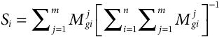
![]() is obtained by addition of m extent analysis values in the fuzzified pair wise comparison matrix.
is obtained by addition of m extent analysis values in the fuzzified pair wise comparison matrix.
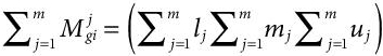
![]() is calculated by fuzzy addition of
is calculated by fuzzy addition of ![]() which is done as:
which is done as:
After calculation of the Si value, the degree of possibility is calculated. If M1 = (l1, m1, u1) and M2 = (l2 ,m2, u)2 are two triangular fuzzy numbers and if M2 ≥ M1 then,
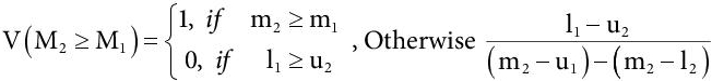
Here, D is the highest point of intersection of µM1 and µM2. Figure 12.1 clearly states that to compare between two Triangular fuzzy numbers M1 and M2, we need both the values V (M1 ≥ M2) & V (M2 ≥ M1 ).
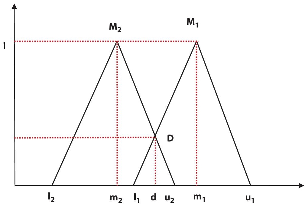
Figure 12.1 Intersection between two triangular fuzzy numbers (M1 & M2).
The degree of possibility of a convex fuzzy numbers to be greater than K convex fuzzy numbers Mi (i= 1, 2, 3,…, k) is given by:
Let d(Ai) = Min V (Si ≥ Sk) for k = 1, 2,3, …,n ; k ≠ i
The weight vector is given by:
where Ai (i = 1, 2, 3, … ,n) are n elements.
Lastly, the weight vectors are normalized to obtain the final weight;
where W is a nonfuzzy number.
In earlier days, profit maximization was the only goal of financial management system. But now, there is no single universal goal. So, goal programming is an approach used for solving such multiple objective prioritized optimization problems.
The approach for formulating goal programming model is same as linear programming model. The decision variables are x1,x2,...,xn first defined.
All specified goals are ranked in order of priority. A general goal programming can be stated as:
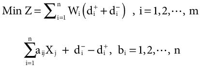
and
When Wi is weight vector calculated by Fuzzy AHP method. ![]() are positive and negative deviations from the ith goal.
are positive and negative deviations from the ith goal.
12.2 Research Model
The model has been developed to estimate the nonperforming assets on certain parameters of State Bank of India (SBI). The NPA of SBI has been broadly distributed among priority sector and nonpriority sector. Both these sectors have been individually classified into agriculture and allied activities, industries (micro and small, medium and large), services, and personal loans. Data of Table 12.1 has been taken from SBI annual report 2019–2020. Table 12.2 has been calculated weight of different criterion by applying fuzzy AHP with the help of Table 12.1. Table 12.3 has prepared by using original Saaty’s scale which citation is provided below [20]. Table 12.4 has been prepared by me using original Saaty’s scale mentioned in Table 12.3. Table 12.5 has been calculate with the help of Table 12.2 by applying Extended Saaty’s scale, as in Table 12.4. Table 12.6 has been prepared using data from audited annual report of SBI from year 2013 to 2020. Then, the dependency of various sectors on gross NPA is calculated by applying fuzzy AHP to find the weights of the different criterion.
Now, the priority comparison matrix is made by simply dividing the percentage value of different criterion. For example, for the cell a12, we have to find how dominant is agricultural NPA over the NPA in industries of priority sectors. Then, we will simply divide the percentage value of gross NPA to total NPA in agricultural sector by the percentage value of gross NPA to total NPA in the industrial sector.
After making the pairwise comparison matrix, the crisp value in the matrix are converted into fuzzy numbers using extension of Saaty’s scale.
Table 12.1 Gross NPA in priority and non-priority sectors.
| Sectors | Outstanding advances (Rs in Crore) | Gross NPA (Rs in Crore) | Percentage of gross NPA to total advances to that sectors |
| A. Priority sectors | |||
| (i) Agriculture and allied activities | 2,04,185.71 | 32,558.27 | 15.95 |
| (ii) Industries (micro and small, medium and large) | 1,01,080.54 | 18,738.88 | 18.54 |
| (iii) Services | 83,870.61 | 5,289.20 | 6.31 |
| (iv) Personal loans | 1,66,800.34 | 3,131.18 | 1.88 |
| Subtotal | 5,55,937.20 | 59,717.53 | 10.74 |
| B. Non-priority sectors | |||
| (i) Agriculture and allied activities | 2,235.29 | 229.81 | 10.28 |
| (ii) Industries (micro and small, medium and large) | 10,54,285.42 | 74,644.63 | 7.08 |
| (iii) Services | 2,21,642.21 | 9,686.06 | 4.37 |
| (iv) Personal loans | 5,88,744.65 | 4,813.82 | 0.82 |
| Subtotal | 18,66,907.57 | 89,314.32 | 4.79 |
| Total (A+B) | 24,22,844.77 | 1,49,091.85 | 6.15 |
Table 12.2 Interdependency of different economic sectors.
| Agriculture and allied activities | Industries (micro and small, medium and large) | Services | Personal | Agriculture and allied activities | Industries (microand small, medium and large) | Services | Personal | |
| Agriculture and allied activities | 1 | 0.860 | 2.527 | 8.484 | 1.551 | 2.252 | 3.649 | 19.451 |
| Industries (micro and small, medium and large) | 1.162 | 1 | 2.938 | 9.861 | 1.803 | 2.618 | 4.242 | 22.609 |
| Services | 0.395 | 0.340 | 1 | 3.356 | 0.613 | 0.891 | 1.443 | 7.695 |
| Personal | 0.117 | 0.101 | 0.297 | 1 | 0.182 | 0.265 | 0.430 | 2.292 |
| Agriculture and allied activities | 0.644 | 0.554 | 1.629 | 5.468 | 1 | 1.451 | 2.352 | 12.536 |
| Industries (micro and small, medium and large) | 0.443 | 0.381 | 1.122 | 3.765 | 0.688 | 1 | 1.620 | 8.634 |
| Services | 0.273 | 0.235 | 0.692 | 2.324 | 0.425 | 0.617 | 1 | 5.329 |
| Personal | 0.051 | 0.044 | 0.129 | 0.436 | 0.079 | 0.115 | 0.181 | 1 |
Table 12.3 Original Saaty’s scale for pairwise comparison.
| Crisp value | Definition | Fuzzified value |
| 1 | Equal importance | (1, 1, 1+δ) |
| 3 | Weak dominance | (3-δ, 3, 3+ δ) |
| 5 | Strong dominance | (5-δ,5,5+ δ) |
| 7 | Demonstrated dominance | (7-δ, 7, 7+ δ) |
| 9 | Absolute dominance | (9-δ, 9, 9+ δ) |
| 2,4,6,8 | Intermediate values | (x-1,x,x+1) ; where x=2,4,6,8 |
δ is fuzzy distance(0.5≥ δ≤ 2).
Table 12.4 Extension of Saaty’s scale.
| Crisp value | Definition | Fuzzified value |
| 1 | Equal importance | (1,1,1+δ) |
| 3 | Weak dominance | (3-δ,3,3+ δ) |
| 5 | - | (5-δ,5,5+ δ) |
| 7 | - | (7-δ,7,7+ δ) |
| 9 | - | (9-δ,9,9+ δ) |
| 11 | - | (11-δ,11,11+ δ) |
| 13 | - | (13-δ,13,13+ δ) |
| 15 | - | (15-δ,15,15+ δ) |
| 17 | - | (17-δ,17,17+ δ) |
| 19 | - | (19-δ,19,19+ δ) |
| 21 | - | (21-δ,21,21+ δ) |
| 23 | - | (23-δ,23,23+ δ) |
| 25 | Absolute Dominance | (25-δ,25,25+ δ) |
Table 12.5 Fuzzified matrix.
| (1, 1, 1.5) | (0.602, 0.861, 1.511) | (2.027, 2.527, 3.027) | (7.984,8.484, 8.984) | (1.051, 1.551, 2.051) | (1.752, 2.252, 2.752) | (3.149, 3.694, 4.149) | (18.951, 19.451, 19.951) |
| (0.002,1.162,1.662) | (1, 1, 1.5) | (2.438, 2.938, 3.438) | (9.361, 9.861, 10.361) | (1.303, 1.803, 2.303) | (2.118, 2.618, 3.118) | (3.742, 4.242, 4.742) | (22.109, 22.609, 23.109) |
| (0.330,0.396,0.493) | (0291, 0.340, 0.410) | (1, 1, 1.5) | (2.856, 3.356, 3.856) | (0.470, 0.614, 0.886) | (0.617, 0.891, 1.608) | (0.943, 1.443, 1.943) | (7.195, 7.695, 8.195) |
| (0.111, 0.118,0.125) | (0.097,0.101, 0.107) | (0.259,0.298, 0.350) | (1, 1, 1.5) | (0.168, 0.183, 0.201) | (0.234, 0.266, 0.306) | (0.354, 0.430, 0.548) | (1.792, 2.292, 2.792) |
| (0.488,0.645,0.951) | (0.434, 0.555, 0.767) | (1.129, 1.629, 2.129) | (4.968, 5.468, 5.968) | (1, 1, 1.5) | (0.951, 1.451, 1.951) | (1.852,2.352,2.852) | (12.036,12.536,13.036) |
| (0.363,0.444,0.571) | (0.321, 0.382, 0.472) | (0.622, 1.122, 1.622) | (3.265, 3.765, 4.265) | (0.513,0.689,1.052) | (1,1,1.5) | (1.120,1.620,2.120) | (8.134,8.634,9.134) |
| (0.241,0.274,0.318) | (0.211, 0.236, 0.267) | (0.515, 0.693, 1.060) | (1.824, 2.324, 2.824) | (0.351,0.425,0.540) | (0.472,0.617,0.893) | (1,1,1.5) | (4.829,5.329,5.829) |
| (0.050,0.051,0.053) | (0.043, 0.044, 0.045) | (0.122, 0.130, 0.139) | (0.358, 0.436, 0.558) | (0.077,0.080,0.083) | (0.109,0.116,0.123) | (0.172,0.188,0.207) | (1,1,1.5) |
With the help of this scale a new fuzzified matrix is created, are as follows in Table 12.5:
Using this fuzzified matrix, fuzzy synthetic extent is calculated. is calculated.
Finally, using equation (12.1) Fuzzy synthetic extent is obtained as:
Here weights have calculated by de-fuzzifying the Si values, i.e., the fuzzy synthetic extent values.
So weights are:
Hence, normalized weights are:
12.2.1 Average Growth Rate Calculation
The average growth rate in different sectors has been calculated using the data of seven years from 2013–2014 to 2019–2020. At first, the percentage increase between two consecutive years is calculated and then the average percentage increase in gross NPA is calculated by taking the mean of the percentage increase of different consecutive years. Table 12.6 shows the average growth rate of different sectors in percentage.
The first group of models input and output variable are taken in Table 12.7.
In Table 12.8, priority arrangement of variables is done as per the normalized weights calculated by Fuzzy AHP.
The linear problem on the basis of obtained weights is discussed below in equation 12.6. The lower limit in different equations has been taken from Table 12.1 from the column of gross NPA. The upper limit in the equation has been obtained by calculating the average percentage increase over gross NPA in 2020. For example, for x, i.e., NPA from industry (priority sector) the gross NPA is taken always greater1 than that in 2020, which is Rs. 18738.88 cr.
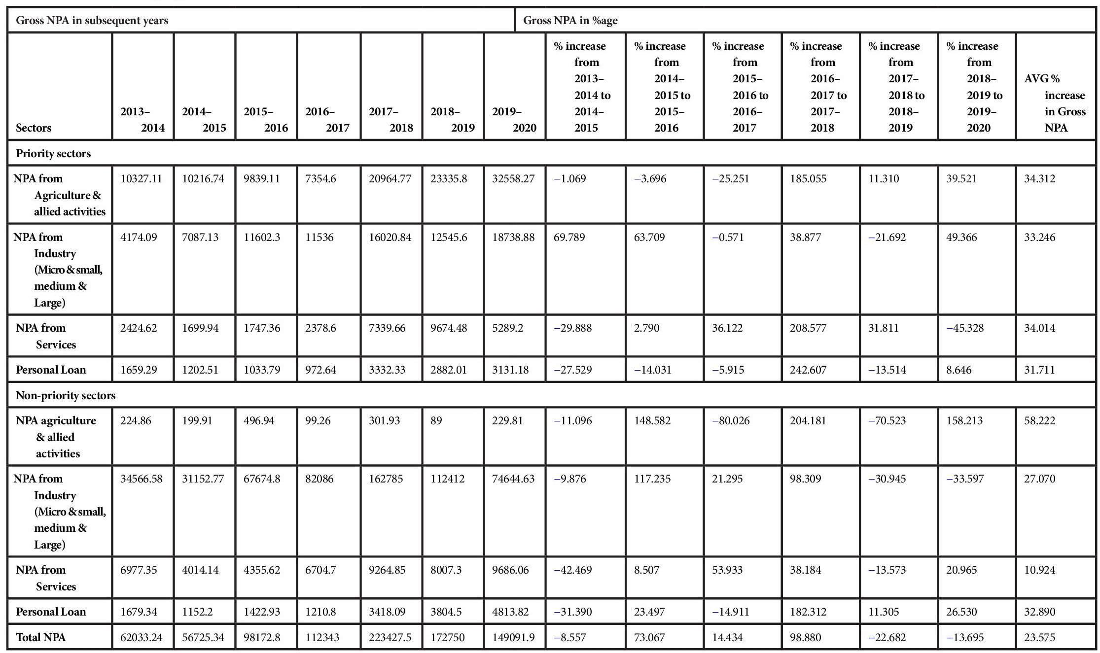
Table 12.6 Average growth rate in different sectors.
Table 12.7 Arrangement of priority and non-priority sectors as per weight.
| Priority sector | Input & output variable | |
| I | NPA from Agriculture & allied activities | X2 |
| II | NPA from Industry (Micro & small, medium & Large) | X1 |
| III | NPA from Services | X5 |
| IV | Personal Loan | X7 |
| Non-priority sector | ||
| V | NPA agriculture & allied activities | X3 |
| VI | NPA from Industry (Micro & small, medium & Large) | X4 |
| VII | NPA from Services | X6 |
| VIII | Personal Loan | X8 |
Table 12.8 Priority arrangement.
| Sectors | Priority weight after normalization | Coefficient | |
| I | NPA from Industry (Micro & small, medium & Large) (priority sector) | X1 | 0.284 |
| II | NPA from Agriculture & allied activities (priority sector) | X2 | 0.243 |
| III | NPA agriculture & allied activities (Non-priority sector) | X3 | 0.157 |
| IV | NPA from Industry (Micro & small, medium & Large) (Non-priority sector) | X4 | 0.110 |
| V | NPA from Services (priority sector) | X5 | 0.097 |
| VI | NPA from Services (Non-priority sector) | X6 | 0.068 |
| VII | Personal Loan (priority sector) | X7 | 0.028 |
| VIII | Personal Loan (Non-priority sector) | X8 | 0.012 |
Now, for the upper limit of x1, average growth rate is 33.246%. Hence,
Similarly, the upper and lower limits for x2, x3, x4, x5, x6, x7, and x8 can be calculated to get equation 12.6.
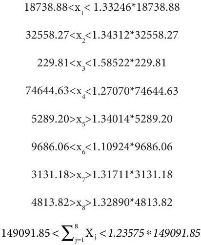
Equivalent goal programming model is as follows:
Here, the coefficients in z have been taken from Table 12.8, which is the normalized weight.
z=0.284*(d1plus)+0.243*(d2plus)+0.157*(d3plus)+0.110* (d4 plus) +0.097 * (d5 plus) +0.068*(d6 plus) +0.028* (d7plus)+0.012*(d8plus)
Outcome recorded after minimizing the Goal programming problem (12.7) using Lingo19 optimization software clearly shows that the global optimal solution is possible as in Figure 12.2.
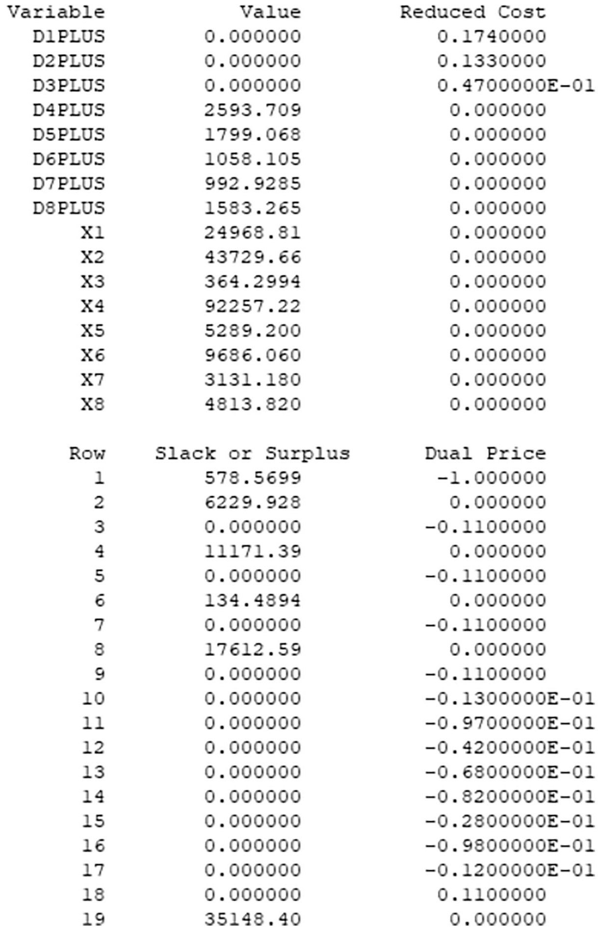
Figure 12.2 Feasibility result of goal programming model.
12.3 Result and Discussion
The proposed model has estimated the NPA of priority and nonpriority sectors which includes agriculture and allied activities, industries (micro and small, medium and large), services and personal loans.
A comparison table result has been mentioned below in Table 12.9, which clearly shows that the NPA in agriculture and allied activities, industries (micro and small, medium and large) and personal loans of both priority and nonpriority sector has shown modest growth but are below the benchmark of the average growth rate as per the model result. However, the NPA in services has almost doubled showing the rapid growth compared to the average growth of the model result.
Table 12.9 Comparison of gross NPA in SBI annual report 2020–2021 to gross NPA as per model result.
| Sectors | Gross NPA in SBI annual report 2020-21 (Rs in Crore) | Gross NPA as per model result (Rs in Crore) |
| Priority sector | ||
| (i) Agriculture & allied activities | 32,392.47 | 43,729.66 |
| (ii) Industries (micro & small, medium & large) | 11,206.95 | 24,968.81) |
| (iii) Services | 10,198.53 | 5,289.200 |
| (iv) Personal loans | 2,352.84 | 3,131.180 |
| Non-priority sector | ||
| (i) Agriculture & allied activities | 205.85 | 364.2994 |
| (ii) Industries (micro & small, medium & large) | 47,770.41 | 92,257.22 |
| (iii) Services | 17,636.56 | 9,686.060 |
| (iv) Personal loans | 4,625.41 | 4813.820 |
| Total | 1,26,389.02 | 184,240.25 |
12.4 Conclusion
In view of the outcome of the proposed model, all eight different goals have been scrutinized and achieved. The findings clearly state that the performance of state bank of India (SBI) is good in agriculture and allied activities, industries (micro and small, medium and large) and personal loans of both priority and nonpriority sector but the NPA of the service sector has doubled with respect to the model result. This shows a serious concern of the bank to work individually on service sector in order to maintain its NPA. The infeasibility for the linear model was overcome by the goal programming model. Furthermore, the developed model can be implemented to prepare a solution system, which can help banks and other financial institutions to design a blueprint. This can further help them to identify their benchmark, which can be achieved in the future.
References
- 1. Charnes, A. and Cooper, W.W., Management models and industrial applications of linear programming. Manage. Sci., 4, 1, 38–91, 1957.
- 2. Aouni, B. and Kettani, O., Goal programming model: A glorious history and a promising future. Eur. J. Oper. Res., 133, 2, 225–231, 2001.
- 3. Zadeh, L.A., Fuzzy sets, in: Fuzzy Sets, Fuzzy Logic, and Fuzzy Systems: Selected Papers, Zadeh, L.A. (Ed.), pp. 394–432, 1996.
- 4. Zimmermann, H.J., Description and optimization of fuzzy systems. Int. J. Gen. Syst., 2, 1, 209–215, 1975.
- 5. Zimmermann, H.J., Fuzzy programming and linear programming with several objective functions. Fuzzy Sets Syst., 1, 1, 45–55, 1978.
- 6. Mohammadi, R. and Sherafati, M., Optimization of bank liquidity management using goal programming and fuzzy AHP. Res. J. Recent Sci., 4, 6, 53–61, 2015.
- 7. Sivrikaya, B.T., Kaya, A., Dursun, M., Çebi, F., Fuzzy AHP–goal programming approach for a supplier selection problem. Res. Logist. Prod., 5, 271– 285, 2015.
- 8. Srdjevic, B. and Medeiros, Y.D.P., Fuzzy AHP assessment of water management plans. Water Res. Manage., 22, 7, 877–894, 2008.
- 9. Pourahmad, A., Hosseini, A., Banaitis, A., Nasiri, H., Banaitienė, N., Tzeng, G.H., Combination of fuzzy-AHP and DEMATEL-ANP with GIS in a new hybrid MCDM model used for the selection of the best space for leisure in a blighted urban site. Technol. Econ. Dev. Econ., 21, 5, 773–796, 2015.
- 10. Yaghoobi, M.A., Jones, D.F., Tamiz, M., Weighted additive models for solving fuzzy goal programming problems. Asia Pac. J. Oper. Res., 25, 05, 715–733, 2008.
- 11. Kumar, M., Vrat, P., Shankar, R., A fuzzy goal programming approach for vendor selection problem in a supply chain. Comput. Ind. Eng., 46, 1, 69–85, 2004.
- 12. Kahraman, C. and Büyüközkan, G., A Combined fuzzy AHP and fuzzy goal programming approach for effective six-sigma project selection. J. Mult.-Valued Log. Soft Comput., 14, 6, 599–615, 2008.
- 13. Vidyasagar, K. and Dwivedi, R.K., Post demonetisation effect on banking sector, micro financing institutions (MFI) and job opportunities. Int. J. Manage. Innov. Entrep. Res., 6, 2, 39–44, 2020, https://doi.org/10.18510/ijmier.2020.624.
- 14. Vekariya, S.P., Can Indian banking industry overcome NPA issue uring the pandemic time? PBME, 103, 103–110.
- 15. Monetary policy report, Reserve Bank of India (RBI), India, April 2020.
- 16. Dave, P. and Joshi, Y.C., NPA and indian banking sector: Assessing the impact on the profitability of public sector banks in India, GH Patel Postgraduate Institute of Business Management, Gujrat, India, 1935.
- 17. Khandelwal, V. and Modi, S., India’s NPA situation with an emphasis on public and private banks, vol. 3857444, SSRN, Haryana, India, 2021.
- 18. Haralayya, D., Study on non performing assets of public sector banks. Iconic Res. Eng. J. (IRE), 4, 12, 52–61, 2021.
- 19. Prasanth, S., Nivetha, P., Ramapriya, M., Sudhamathi, S., Factors affecting non performing loan in India. Int. J. Sci. Technol. Res., 9, 1, 1654–1657, 2020.
- 20. Saaty, T., The analytic hierarchy process (AHP) for decision making, pp. 1–69, Kobe, Japan, 1980.
- 21. Chang, D.Y., Applications of the extent analysis method on fuzzy AHP. Eur. J. Oper. Res., 95, 3, 649–655, 1996.
Note
- * Corresponding author: [email protected]