
1
Band Reduction of HSI Segmentation Using FCM
V. Saravana Kumar1*, S. Anantha Sivaprakasam2, E.R. Naganathan3, Sunil Bhutada1 and M. Kavitha4
1 Department of IT, SreeNidhi Institute of Science and Technology, Hyderabad, India
2 Department of CSE, Rajalakshmi Engineering College, Chennai, India
3 Department of CSE, Koneru Lakshmaiah Education Foundation, Vaddeswaram, AP, India
4 Research Scholar, Manonmaniam Sundaranar University, Tirunelveli, India
Abstract
Hyperspectral has carried hundreds of nonoverlapping spectral channels of a specified scene, clustering is one of the approaches for diminishing the size of these large data sets. Segmentation is intricate for the raw data; however, it is likely for the reduced band of HSI. To lessen the band size, the classical clustering methods for example K-means, Fuzzy C-means are accomplished. An integrated image segmentation procedure built on interband clustering and intraband clustering is proposed. The interband clustering is performed by K-means clustering and Fuzzy C-means clustering algorithms, despite the fact the intraband clustering is executed using particle swarm segmentation (PSO) clustering algorithm. The performance of the K-means algorithm is subject to initial cluster centers. Besides, the final partition should be contingent on the initial configuration. The clustering consequences have profoundly been subject to the number of clusters stated. It is essential to provide refined direction for defining the number of clusters with the purpose of attaining appropriate clustering consequences. Davies Bouldin (DB) index is one of the reliable methods to outline the number of clusters for these clustering methods. The hyperspectral bands are clustered, and a band which has extreme variance from each cluster is preferred. This tactic forms the diminished set of bands. PSC (EEOC) accomplishes the segmentation process on the reduced bands. In conclusion, there is a comparison of the result produced for K-means worked with EEOC and FCM worked with EEOC in various HSI scenes.
Keywords: K-means, Fuzzy C-means, band reduction, PSO, cluster, centroid
1.1 Introduction
Hyperspectral [14] has carried hundreds of nonoverlapping spectral channels [11] of a given scene, clustering [13, 21] is one of the methods for reducing the size of these large data sets. Despite displaying the size of hyperspectral scene [17], the device does not support to display the scene directly. Segmentation is complicated for the raw data, whereas it is possible for the reduced band scene. Even though hyperspectral data [3] can provide finely resolved details about the spectral properties [4] to be identified, it also has some limitation. When dealing with such high-dimensional data [24, 25], one is faced with the “curse of dimensionality” problem One popular way to tackle the curse of dimensionality [7] is to employ a feature extraction technique [22]. To diminish the band size, the classical clustering methods [30], such as K-means, Fuzzy C-means [27] are handled. The former can be sensitive to the initial centers, while the results from the latter depend on the initial weights. Here, an integrated image segmentation [2] process based on interband clustering and intraband clustering is proposed. The interband clustering is performed by K-means clustering or Fuzzy C-means clustering algorithms, whereas the intraband clustering is executed using particle swarm segmentation (PSO) clustering algorithm. The performance of the K-means algorithm depends on initial cluster centers. Besides, the final partition depends on the initial configuration. The clustering results have heavily depended on the number of clusters specified. It is necessary to provide educated guidance for determining the number of clusters in order to achieve appropriate clustering results. Davies Bouldin (DB) index is one of the reliable methods to determine the number of clusters for these clustering methods. The hyperspectral bands [18] are clustered and a band [34], which has maximum variance, from each cluster is chosen. This forms the reduced set of bands. PSC (EEOC) [29] performs the segmentation process on the reduced bands. Finally, the result produced from K-means worked with EEOC and FCM worked with EEOC in various HSI [19] scenes was compared.
1.2 Existing Method
1.2.1 K-Means Clustering Method
Theoretically, K-means [1] is a typical algorithm. Now that it is elementary and expeditious, it is attractive in practice. To begin with, it segregates the input dataset into K-lusters. Each cluster is described by an adaptively changing centroid, starting from some initial values named seed points. K-means enumerates the squared distances between the inputs and centroids, and assigns inputs to the nearest centroid. The procedure continues until there is no significant change in the location of class mean vectors between successive iteration of the algorithms. Apparently, the performance of the K-means algorithm depends on initial cluster centers, whereas the final partition depends on the initial configuration.
1.2.2 Fuzzy C-Means
In Fuzzy C-means clustering [8], data elements can belong to more than one cluster and associated with each element is a set of membership levels. FCM clustering [9] is a process of assigning these membership levels, and then using them to assign data elements to one or more clusters. The aim of FCM [10] is to minimize an objective function. Contrary to traditional clustering analysis methods, which distribute each object to a unique group, fuzzy clustering algorithms gain membership values between 0 and 1 that indicate the degree of membership for each object to each group. Obviously, the sum of the membership values for each object to all the groups is definitely equal to 1. Different membership values show the probability of each object to different groups.
The main limitation of the FCM algorithm [16] is its sensitivity to noise. The FCM algorithm implements the clustering task for a data set by minimizing an objective-function subject to the probabilistic constraint that the summation of all the membership degrees of every data point to all clusters must be one. This constraint results in the problem of this membership assignment, that noise is treated the same as points close to the cluster centers. However, in reality, these points should be assigned very low or even zero membership in either cluster.
Like K-means, the clustering results have heavily depended on the number specified. It is also necessary to provide an educated guidance for determining the number cluster in order to achieve appropriate clustering results. Davies Bouldin (DB) index is one of the reliable methods to determine the number of clusters for these clustering methods.
1.2.3 Davies Bouldin Index
Davies Bouldin index was introduced in 1979 by David L. Davies and Donald W. Bouldin. It is one of the methods for evaluating clustering algorithms. This is an internal evaluation scheme, where the validation of how well the clustering has done using quantities and features inherent to the dataset.
Many other distance metrics can be used, in the case of manifolds and higher dimensional data, where the Euclidean distance may not be the best measure for determining the clusters. It is important to note that this distance metric has to match with the metric used in the clustering scheme itself for meaningful results.
Davies-Bouldin (DB) index is dependent both on the data, as well as the algorithm. The Davies–Bouldin index measures the average of similarity between each cluster and its most similar one. As the clusters have to be compact and separated the lower Davies-Bouldin index produces a better cluster configuration.
In this work, the interband clustering and intraband clustering approach has proposed. In interband clustering part; existing method such as K-means and Fuzzy C-means method are applied to reduce the band size. In intraband clustering part; a lightweight algorithm, namely Enhanced Estimation of Centroid (EEOC) [33] is proposed. This method is examined with the abovementioned clustering method by applying in various hyperspectral scenes.
1.2.4 Data Set Description of HSI
The dataset contains a variety of hyperspectral remote sensing [15], which are acquired from airborne and satellite. In this work, certain data, such as Salinas A, Salinas Valley, Indian Pines, Pavia University, and Pavia Centre, are handled.
The original scene and its corresponding ground truth image are downloaded from the link. http://www.ehu.eus/ccwintco/index.p...Hyperspectral_Remote_Sensing_Scenes
These scenes are a widely used benchmark for testing the accuracy of hyperspectral data [20] classification [23, 26] and segmentation [31].
1.3 Proposed Method
1.3.1 Hyperspectral Image Segmentation Using Enhanced Estimation of Centroid
These topics explain the integration of intraband and interband cluster approach for segmentation of hyperspectral image in a synergistic fashion. It demonstrates the advantage of the advanced properties of both analysis techniques in combined fashion of clustering method. The ultimate goal is to improve the analysis and interpretation of hyperspectral image. Owing that, classifications [5, 12], as well as segmentation [6], face problems related to the extremely high dimensionality [32] of the hyperspectral images are dominated by mixed pixels and un-mixing techniques are crucial for a correct interpretation and exploitation of the data. This chapter explored the integration of intraband and interband clustering methods for segmentation process with the ultimate goal of obtaining more accurate methods for the analysis of hyperspectral scene without increasing significantly the computational complexity of the process. There are many things to do for achieving this goal; to begin with, to improve unsupervised segmentation [28] by learning a task-relevant measure of spectral similarity from the feature matrix approaches. Besides, interband and intraband cluster techniques for segmentation are proposed. In addition, various existing clustering techniques are applied to interband part. Moreover, for improving the accuracy of various clustering methods, Davies-Bouldin Index is used to determine the number of clusters.
Furthermore, for intraband cluster, a new and novel algorithm entitled as Enhanced Estimation of Centroid (EEOC), which is the modification of the particle swarm clustering method, is proposed. The modification is that the particle has updated their positions and computed the distance matrix only once per iteration. In addition, performances about these methods are evaluated in different scenarios. Performance measurements are used in this research to investigate the efficacy of this system.
The working principle of hyperspectral image segmentation using EEOC is depicted in Figure 1.1. To begin with, the hyperspectral scene in the form of mat file is read; the feature matrix could be constructed based on mean or median absolute deviation (MAD), standard deviation (STD), variance (VAR). In addition, apply one of the clustering processes, namely K-means or Fuzzy C-means. Since these clustering method works depend on the number of cluster, Davies Bouldin (DB) index is used to determine the number of clusters. Furthermore, the dimensional reduction process could be carried out by this clustering method by picking out one band from each cluster, such as 204 bands of hyperspectral image are reduced to below twenty bands, i.e., one band is pick out based on maximum variance from each cluster. In particle swarm clustering algorithm, the input is reduced set of bands from K-means or FCM clustering algorithm. PSC (EEOC) is used for segmentation on the reduced bands.
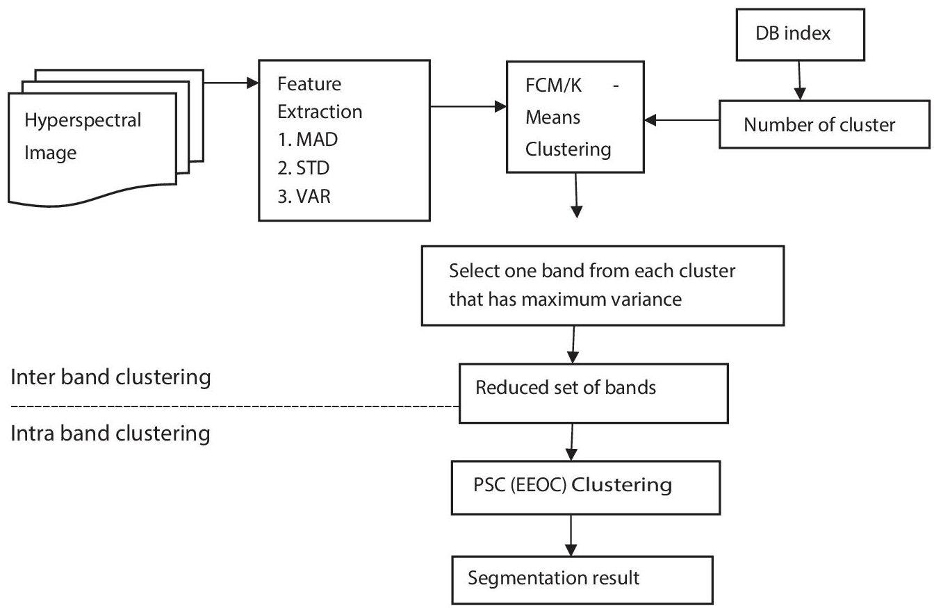
Figure 1.1 Flowchart for hyperspectral image segmentation using EEOC.
1.3.2 Band Reduction Using K-Means Algorithm
K-means is an iterative technique that is used to partition the hyperspectral feature matrix into K clusters. It is one of the simplest unsupervised learning algorithms to solve the well-known clustering problem. The aim of this method is to minimize the sum of squared distances between all points and the cluster center.
The K-means algorithm is reduced the hyperspectral feature matrix is shown in Figure 1.2. Get the hyperspectral feature matrix and the number of clusters (determined from DB Index). Choose the K initial cluster centers, after which the new cluster is computed, 204 bands of the hyperspectral matrix are reduced to 17 bands, i.e., one band is selected according to the maximum variance from each cluster. Finally, the reduced set of bands is obtained.
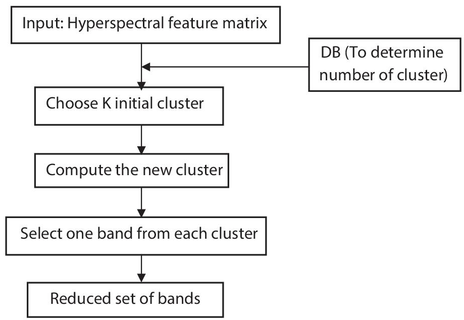
Figure 1.2 Band reduction using K-means algorithm.
1.3.3 Band Reduction Using Fuzzy C-Means
Fuzzy C-means is an iterative technique that is used to partition the hyperspectral feature matrix into membership levels. Data elements can belong to more than one cluster in this method and associated with each element in a set of membership levels. It is a process of assigning these membership levels and then using them to assign data elements to one or more clusters.
The Fuzzy C-means algorithm is reduced the hyperspectral feature matrix is as abovementioned Figure 1.3. Get the hyperspectral feature matrix and the number of clusters that determine the DB Index. The membership matrix is initialized after which fuzzy cluster is calculated. Then, membership matrix is updated. 204 bands of the hyperspectral matrix are reduced to 17 bands i.e. one band is selected according to the maximum variance from each cluster. Finally, the reduced set of bands is obtained. The above flowchart shows the flow of band reduction using Fuzzy C-means clustering algorithm.
By using this above said clustering method, the hyperspectral bands are reduced into below 20 bands, depending on the scene. The DB index helps to determine the number of clusters, based on this number of cluster the bands are reduced, i.e., applying this clustering method into the hyperspectral feature matrix. These matrices are clusters that depend on the number of clusters. Then, pick out one band from each cluster, which has a maximum variance, i.e., number of clusters is 18, that implies the maximum variance band is pick out from each cluster and thus this hyperspectral data are reduced into 18 bands. This reduced band is allowed to segmentation, which is carried out by a light weight clustering algorithm. This algorithm is entitled as enhanced estimation of centroid (EEOC), which is the modification of the particle swarm clustering method performed. The modification is that the particle has updated their positions and computed the distance matrix only once per iteration.

Figure 1.3 Band reduction using Fuzzy C-means.
1.4 Experimental Results
The performance of EEOC algorithm is analyzed and experimented. Its performance is noticed to be satisfactory in term of reduction in the time complexity and the efficiency of each position update.
1.4.1 DB Index Graph
Figure 1.4(a) depicts DB Index Graph. In x-axis, number of clusters (i.e., the value is incremented by 1 pixel) and in y-axis, DB value (i.e., the value is increment by 0.05 pixels) is determined.
For Salinas_A scene, the DB-value is least at 17th cluster. So, the DB Index of this scene is considering as 17. For Indian Pines the DB value is least at 11th cluster. So, the DB Index is considered as 11 for this scene. For Salinas Valley Scene, the DB value is least at 10th cluster. So, the DB Index is considered as 10 for this scene. For Pavia University, the DB value is least at 20th cluster. So, the DB Index is considered as 20 for this scene. For Pavia Centre Scene, the DB value is least at 19th cluster. So, the DB Index is considered as 19 for this scene.
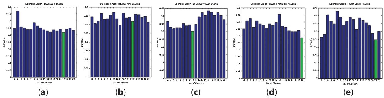
Figure 1.4 DB Index Graph. (a) Salina_A scene (b) Indian Pines (c) Salinas Valley (d) Pavia University and (e) Pavia Center scene.
1.4.2 K-Means–Based PSC (EEOC)
Figure 1.5(a) shows the segmentation result for the hyperspectral scene, namely Salinas_A, is processed by K-means based PSC (EEOC). In the interband clustering, K-means is utilized to reduce the band, whereas PSC (EEOC) is performed in intracluster. For this reason this approach is named as K-means based PSC (EEOC). Figures 1.6(a), 1.7(a), 1.8(a), 1.9(a) portrays the segmentation results for the hyperspectral scenes, namely Indian Pines, Salinas Valley, Pavia University, and Pavia Center, respectively. The pixels, which are clustered based on K-means working with PSC (EEOC), are displayed in Table 1.1.
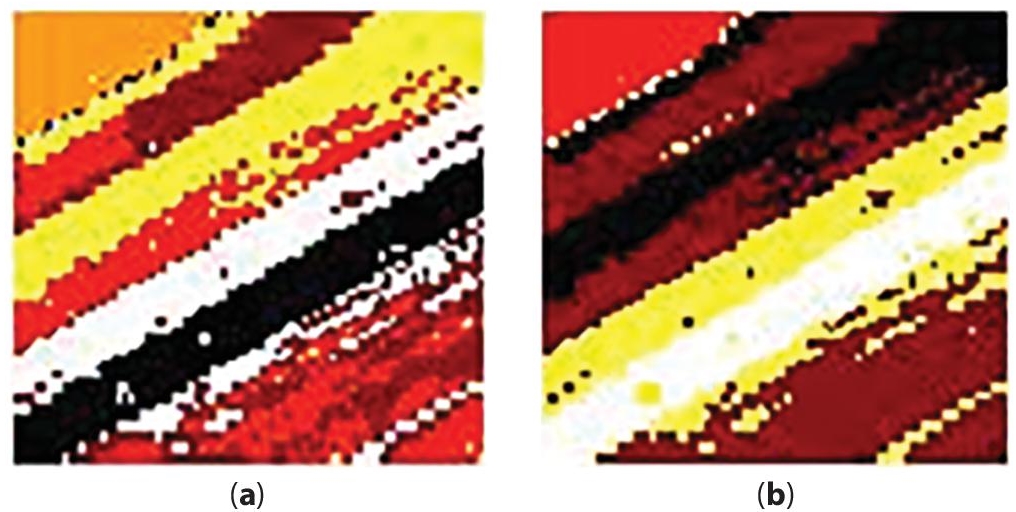
Figure 1.5 Results for Salinas_A, (a) K-means + PSC (EEOC) (b) FCM + PSC (EEOC).
Table 1.1 Pixels clustered based on PSC (EEOC) with K-means and FCM for Salinas_A.
| SALINAS _A 83 × 86 × 204 | Clusters | K–Means + PSC (EEOC) | FCM + PSC (EEOC) |
| Pixels | Pixels | ||
| 1 | 1284 | 1371 | |
| 2 | 1492 | 2788 | |
| 3 | 1081 | 507 | |
| 4 | 611 | 1 | |
| 5 | 507 | 1431 | |
| 6 | 2163 | 1040 |
1.4.3 Fuzzy C-Means–Based PSC (EEOC)
Figures 1.5(b), 1.6(b), 1.7(b), 1.8(b), and 1.9(b) portray the segmentation results for FCM based on PSC (EEOC), which is examined on this HSI. The pixels are clustered based on FCM +PSC (EEOC) is listed in Table 1.1.
The following figures (Figures 1.5 to 1.9), left side images (a images), depict the results for K-means working with PSC (EEOC) of the various hyperspectral scenes. The right side listed images (b images) portray the results for FCM working with PSC (EEOC).
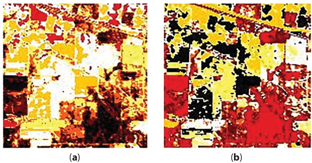
Figure 1.6 Results for Indian Pines (a) K-means + PSC (EEOC) (b) FCM +PSC (EEOC).
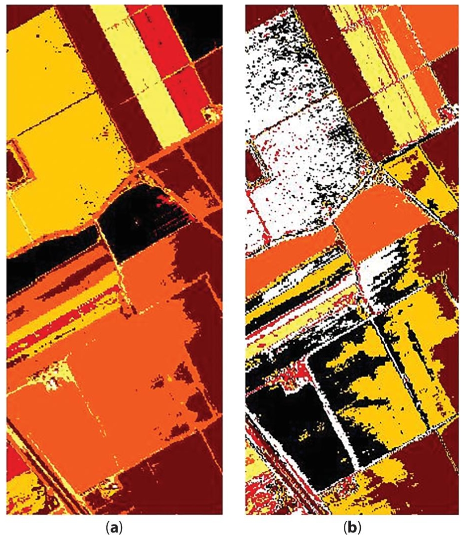
Figure 1.7 Results for Salinas Valley. (a) K-means + PSC (EEOC) (b) FCM + PSC (EEOC).
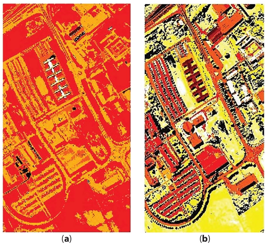
Figure 1.8 Results for Pavia University. (a) K-means + PSC (EEOC) (b) FCM + PSC (EEOC).
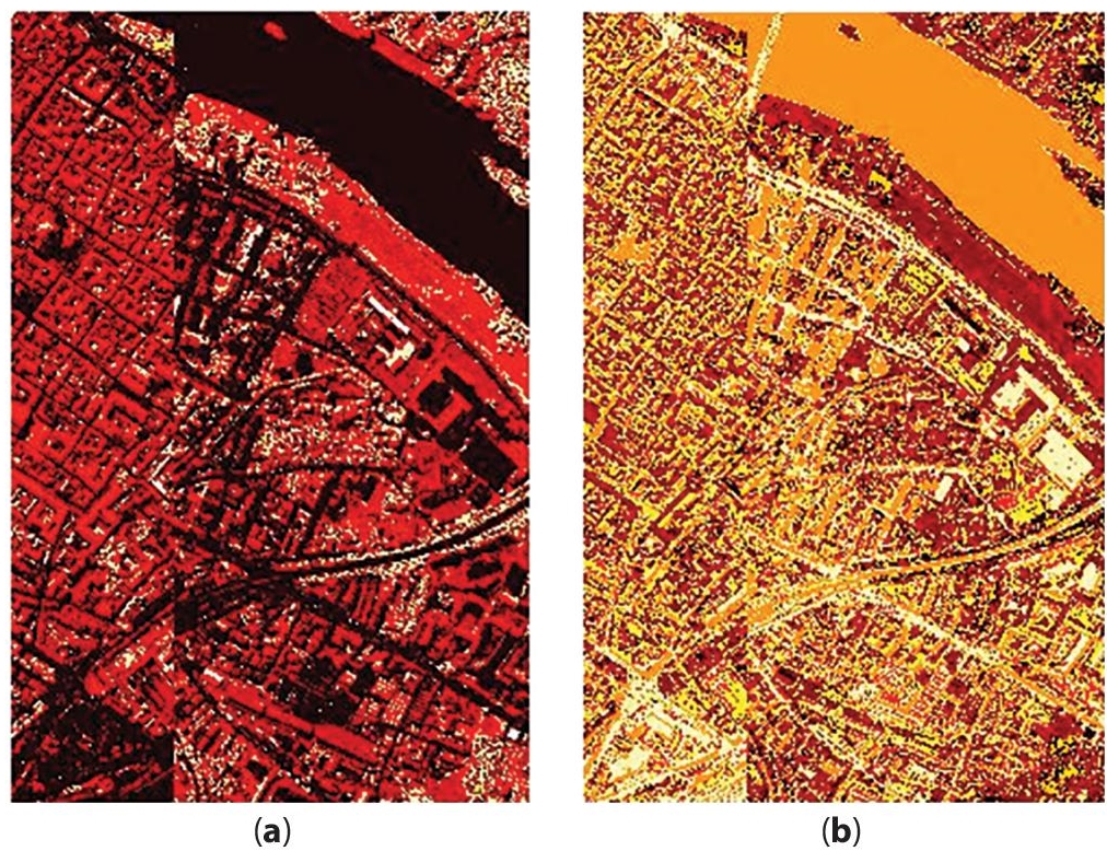
Figure 1.9 Results for Pavia Centre. (a) K-means + PSC (EEOC) (b) FCM + PSC (EEOC).
1.5 Analysis of Results
The following tables illustrate the resultant of the number of pixels, which are clustered. The number of the cluster is defined based on the ground truth, as well as important features of the abovementioned HSI.
Table 1.1 depicts the result of performance based on pixel wise cluster for the Salinas_A scene. As per the reference of the ground truth image, Salinas_A scene has segmented with six clusters. The size of this scene is 83 × 86 × 204. The 204 bands are reduced into 17 bands as per the Davies– Bouldin Index and finally this 83 x 86 pixels are clustered into six, such as 7138 pixels are grouped into these clusters. From Table 1.1, K-means working with PSC (EEOC) clustered the pixels equally, whereas 4th cluster has one pixel for FCM.
Table 1.2 portrays the result of performance based on pixel wise cluster for the Indian Pines scene. As per the reference of the ground truth image, the Indian Pines scene has segmented with seven clusters. The size of this scene is 145 × 145 × 200. The 200 bands are reduced into 11 bands as per the Davies-Bouldin Index and finally this 145 × 145 pixels are clustered into seven, such as 21,025 pixels are grouped into these clusters.
Table 1.3 portrays the result of performance based on pixel wise cluster for the Salinas Valley scene. As per the reference of the ground truth image, this scene has segmented with seven clusters. The size of this scene is 512 × 217 × 204. The 204 bands are reduced into 10 bands as per the Davies-Bouldin Index and finally this 512 × 217 pixels are clustered into seven, and 111,104 pixels are grouped into these clusters.
Table 1.2 Pixels clustered based on PSC (EEOC) with K-means and FCM for Indian Pines.
| Indian Pines 145 × 145 × 200 | Clusters | K-Means + PSC (EEOC) | FCM + PSC (EEOC) |
| Pixels | Pixels | ||
| 1 | 2035 | 3354 | |
| 2 | 2953 | 3522 | |
| 3 | 1393 | 3700 | |
| 4 | 3177 | 1497 | |
| 5 | 2662 | 2193 | |
| 6 | 3597 | 3603 | |
| 7 | 5208 | 3156 |
Table 1.3 Pixels clustered based on PSC (EEOC) with K-means and FCM for Salinas Valley.
| Salinas Valley 512 × 217 × 204 | Clusters | K–Means + PSC (EEOC) | FCM + PSC (EEOC) |
| Pixels | Pixels | ||
| 1 | 9006 | 22894 | |
| 2 | 29424 | 21034 | |
| 3 | 6695 | 5021 | |
| 4 | 35776 | 11939 | |
| 5 | 23797 | 18292 | |
| 6 | 6328 | 7784 | |
| 7 | 78 | 24140 |
Table 1.4 portrays the result of performance based on pixel wise cluster for the Pavia University scene. As per the reference of the ground truth image, this scene has segmented with nine clusters. The size of this scene is 610 × 340 × 103. The 103 bands are reduced into 20 bands as per the DB-Index, and finally these 610 × 340 pixels are clustered into nine, such as 207,400 pixels are grouped into these clusters.
Table 1.5 portrays the results of performance based on pixel wise cluster for the Pavia Centre scene. As per the reference of the ground truth image, Pavia Centre scene has segmented with nine clusters. The size of this scene is 1096 × 715 × 102. These 102 bands are reduced into 17 clusters, as per the Davies-Bouldin Index and finally this 1096 × 715 pixels are clustered into six, such as 783640 pixels are grouped into these clusters.
Table 1.6 depicted the time taken for execution of these methods. These approaches are applying on the above said hyperspectral scenes. From the table, K-means + PSC method takes minimum time to execute for all HSI, whereas FCM + PSC method takes more time for processed.
Table 1.4 Pixels clustered based on PSC (EEOC) with K-means and FCM for Pavia University.
| Pavia University 610 × 340 × 103 | Clusters | K-Means + PSC (EEOC) | FCM + PSC (EEOC) |
| Pixels | Pixels | ||
| 1 | 2176 | 104374 | |
| 2 | 656 | 4899 | |
| 3 | 637 | 162 | |
| 4 | 116561 | 23482 | |
| 5 | 13031 | 1013 | |
| 6 | 72789 | 53200 | |
| 7 | 128 | 2150 | |
| 8 | 610 | 2769 | |
| 9 | 812 | 15351 |
Table 1.5 Pixels clustered based on PSC (EEOC) with K-means and FCM for Pavia Centre.
| Pavia Center 1096 × 715 × 102 | Clusters | K –Means + PSC (EEOC) | FCM + PSC (EEOC) |
| Pixels | Pixels | ||
| 1 | 454182 | 38,965 | |
| 2 | 22 | 156,770 | |
| 3 | 52534 | 88,386 | |
| 4 | 26 | 63,542 | |
| 5 | 130076 | 194,464 | |
| 6 | 9294 | 13,021 | |
| 7 | 132714 | 115,264 | |
| 8 | 20 | 113,205 | |
| 9 | 4772 | 23 |
Table 1.6 Elapsed time in seconds for PSC (EEOC) with K-means and FCM.
| Input | Size | K-means + PSC (EEOC) | FCM + PSC (EEOC) |
| SALINAS_A | 83 × 86 × 204 | 85.4219s | 102.5313s |
| INDIAN PINES | 145 × 145 × 200 | 95.6563s | 104.6719s |
| SALINAS VALLEY | 512 × 217 × 204 | 277.8438s | 283.7031s |
| PAVIA UNIVERSITY | 610 × 340 × 103 | 9.98e+02s | 10.48e+2s |
| PAVIA CENTER | 1096 × 715 × 102 | 19.68e+2s | 18.11e+2s |
Since, in these works, particle swarm clustering method is used, fitness value is one of the parameters to measure the accuracy. The least fitness value indicates the optimum results.
Table 1.7 depicts that the fitness value of EEOC worked with K-means/FCM. PSC (EEOC) worked with FCM produce least fitness value other than the Salinas_A scene. This scene majorly contains the straight line. For this reason, EEOC worked with K-means produce optimum results. In addition, here, it is to be noted that the fitness value for K-means + PSC (EEOC) is a nearby triple of FCM + PSC (EEOC) for Pavia University. For Pavia Centre, the fitness value of FCM + PSC (EEOC) is more than double of K-means + PSC (EEOC). As a whole, EEOC is producing optimum results when worked with the abovementioned clustering methods.
Table 1.7 Fitness value for PSC (EEOC) with K-means and FCM.
| Input | K-means + PSC (EEOC) | FCM + PSC (EEOC) |
| SALINAS_A | 15.99e+5 | 17.96e+05 |
| INDIAN PINES | 96.17e+5 | 92.11e+05 |
| SALINAS VALLEY | 52.38e+6 | 40.82+06 |
| PAVIA UNIVERSITY | 174.56e+6 | 73.65e+06 |
| PAVIA CENTER | 34.16e+07 | 88.72e+07 |
1.6 Conclusions
An integrated image segmentation process based on interband clustering and intraband clustering is proposed. EEOC is used for segmentation process on the reduced bands. The hyperspectral bands are clustered, and a band which has a maximum variance from each cluster is chosen. K-means and FCM are used for interband clustering part, i.e., reduced the band. The Davies-Bouldin Index is used to determine the number of clusters. Finally, reduced set of bands are obtained. PSC (EEOC) takes the reduced set of bands as input and produces the segmentation result.
To be crisp, FCM-based PSC (EEOC) has shown promising results when compared to K-means–based PSC (EEOC) for Salinas Valley, Indian Pines, and Pavia university scenes. Despite producing higher accuracy, FCM clustering takes more time for computation. K-means + PSC (EEOC) clustering produced close results to FCM + PSC (EEOC) clustering for Salinas Valley and Indian Pines. For Pavia University, crystal clearly FCM + PSC (EEOC) produces better results in terms of fitness value and accuracy. As a result, EEOC shows best performance when worked with K-means and Fuzzy C-means clustering method.
References
- 1. Abel Guilhermino da, S., Filho, A.C.F. et al., Hyperspectral images clustering on reconfigurable hardware using the K-means algorithm, in: Integrated circuit and system design, IEEE, US, 2003.
- 2. Sivaprakasam, A., Naganathan, E.R., Saravanakumar, V., Wavelet based cervical image segmentation using morphological and statistical operations. J. Adv. Res. Dyn. Control Syst., 10-03, 1138–1147, 2018.
- 3. Benhalouche, F.Z., Karoui, M.S., Deville, Y., Boukerch, I., Ouamr, A., Multi-sharpening hyperspectral remote sensing data by multiplicative joint-criterion linear-quadratic nonnegative matrix factorization. 2017 IEEE International Workshop of Electronics, Control, Measurement, Signals and their Application to Mechatronics (ECMSM), Donostia-San Sebastian, 2017, pp. 1–6, 2017.
- 4. Song, B., Li, J., Mura, M.D. et al., Remotely sensed image classification using sparse representations of morphological attribute profiles. IEEE Trans. Geosci. Remote Sens., 52, 5122–5136, 2014.
- 5. Bouziani, M. et al., Rule-based classification of a very high resolution image in an urban environment using multispectral segmentation guided by cartographic data. IEEE Trans. Geosci. Remote Sens., 48, 3198–3211, 2010.
- 6. Chen, T.W. et al., Fast image segmentation based on K-means clustering with histograms in HSV color space. Multimedia Signal Processing, IEEE 10th Workshop on, pp. 322–325, 20082008.
- 7. Honga, D., Yokoya, N., Chanussot, J., Xu, J., Zhu, X.X., Learning to propagate labels on graphs: An iterative multitask regression framework for semi-supervised hype-rspectral dimensionality reduction. ISPRS J. Photogramm. Remote Sens., 158, 35–49, 2019.
- 8. Li., D.-F., Linear programming models and methods of matrix games with payoffs of triangular fuzzy numbers, Springer, Berlin, Heidelberg, 2016.
- 9. Li, D.-F., Decision and game theory in management with intuitionistic fuzzy sets, Springer, Heidelberg, Germany, 2014.
- 10. Fan, J. et al., Single point iterative weighted fuzzy C-means clustering algorithm for remote sensing image segmentation. Pattern Recognit., 42, 2527– 2540, 2009.
- 11. Ferraris, V., Dobigeon, N., Wei, Q., Chaber, M. et al., Detecting changes between optical images of different spatial and spectral resolutions: A fusion-based approach. IEEE Trans. Geosci. Remote Sens., 56, 3, 1566– 1578, 2018.
- 12. Gao Yan, J., Mas B, F., Maathuis, H.P., Xiangmin, Z., Van Dijk, P.M., Comparison of pixel-based and object-oriented image classification approaches— A case study in a coal fire area“, Wuda, Inner Mongolia, China. Int. J. Remote Sens., 27, 18, 4039–4055, 20 September 2006.
- 13. Ghosh, A. et al., “Fuzzy clustering algorithms for unsupervised change detection in remote sensing images“. Inform. Sci., 181, 699–715, 2011.
- 14. Govender, M., Chetty, K., Bulcock, H., A review of hyperspectral remote sensing and its application in vegetation and water resource studies. Water SA, 33, 145–151, 2007.
- 15. Guo, B. et al., Customizing kernel functions for SVM-based hyperspectral image classification. Image Process. IEEE Trans., 17, 622–629, 2008.
- 16. An, J.-J. and Li, D.-F., A linear programming approach to solve constrained bi-matrix games with intuitionistic fuzzy payoffs. Int. J. Fuzzy Syst., 21, 3, 908–915, 2019.
- 17. Kerekes, J.P. and Baum, J.E., Hyperspectral imaging system modeling. Linc. Lab. J., 14, 117 –130, 2003.
- 18. Benediktsson, J.A., Palmason, J.A., Sveinsson, J.R., Classification of hyperspectral data from urban areas based on extended morphological profiles. IEEE Trans. Geosci. Remote Sens., 43, 3, 480–491, 2005.
- 19. Bioucas-Dias, J.M. and Plaza, A., Hyperspectral remote sensing data analysis and future challenges. IEEE Geosci. Remote Sens. Mag., 1, 2, 6–36, June 2013.
- 20. Jung., A., Kardevan, P., Tokei, L., Detection of urban effect on vegetation in a less built-up Hungarian city by hyperspectral remote sensing. Phys. Chem. Earth, 30, 255–259, 2005.
- 21. Kavitha, M. et al., Enhanced clustering technique for segmentation on dermoscopic images. IEEE - 4th International Conference on Intelligent Computing and Control Systems (ICICCS 2020), Madurai, TN, pp. 956–961, 2020May 2020.
- 22. Li, Z., Nie, F., Chang, X., Yang, Y., Zhang, C., Sebe, N., Dynamic affinity graph construction for spectral clustering using multiple features. IEEE Trans. Neural Netw. Learn. Syst., 29, 12, 6323–6332, 2018.
- 23. He, L., Chen, X., Li, J., Xie, X., Multiscale super pixel wise locality preserving projection for hyperspectral image classification. MDPI Appl. Sci., 27, 2161, 1-21, May 2019.
- 24. Liu, L., Nie, F., Wiliem, A., Li, Z., Zhang, T., Lovell, B.C., Multi-modal joint clustering with application for unsupervised attribute discovery. IEEE Trans. Image Process., 27, 9, 4345–4356, 2018.
- 25. Khodadadzadeh, M., Li, A.P., Ghassemian, H., Bioucas -Dias, J.M., Li, X., Spectral–spatial classification of hyperspectral data using local and global probabilities for mixed pixel characterization. IEEE Trans. Geosci. Remote Sens., 52, 10, 6298–6314, 2014.
- 26. Pooja, K., Nidamanuri, R.R., Mishra, D., Multi-scale dilated residual convolutional neural network for hyperspectral image classification. 10th Workshop on Hyperspectral Imaging and Signal Processing: Evolution in Remote Sensing (WHISPERS), Amsterdam, Netherlands, pp. 1–5, 2019.
- 27. Saravanakumar, V., Kavitha, M. et al., Fuzzy C-means technique for band reduction and segmentation of hyperspectral satellite image. Int. J. Fuzzy Syst. Appl. (IJFSA), 10, Article 5, 4, 79–100, 2021Sep 2021.
- 28. Saravanakumar, V., Kavitha, M. et al., Robust K-means technique for band reduction of hyperspectral image segmentation, in: Application of hybrid metaheuristic algorithms for image processing, vol. 890, pp. 81–104, Springer – Studies In Computational Intelligence, Switzerland AG, 2020.
- 29. Saravanakumar, V. and Naganathan, E.R., Hyperspectral image segmentation based on enhanced estimation of centroid with fast k-means. Int. Arab J. Inform. Technol. Jordon, 15, 5, 904–911, 2018.
- 30. Saravana Kumar., V., Kavitha, M. et al., Segmentation of hyperspectral satellite image based on classical clustering method. Int. J. Pure Appl. Math., 118, 9, 813–820, 20182018.
- 31. SaravanaKumar., V. and Naganathan, E.R., Segmentation of hyperspectral image using JSEG based on unsupervised clustering algorithms. ICTACT J. Image Video Process., 06, 02, 1152–1158, 2015.
- 32. SaravanaKumar., V. and Naganathan., E.R., A survey of hyperspectral image segmentation techniques for multiband reduction. AJBAS, 9, 7, 226 – 451, 2015.
- 33. SaravanaKumar., V., Naganathan., E.R. et al., Multiband Image Segmentation by using Enhanced Estimation of Centroid (EEOC). Int. Interdiscip. J., Tokyo, Japan, 17- A, 1965–1980, July 2014.
- 34. Yang, H. et al., Unsupervised hyperspectral band selection using graphics processing units. IEEE J. Appl. Earth Observ. Remote Sens., 4, 660–668, 2011.
Note
- * Corresponding author: [email protected]