Mark Colbert University of Central Florida
Jaroslav Křivánek Czech Technical University in Prague
High-fidelity real-time visualization of surfaces under high-dynamic-range (HDR) image-based illumination provides an invaluable resource for various computer graphics applications. Material design, lighting design, architectural previsualization, and gaming are just a few such applications. Environment map prefiltering techniques (Kautz et al. 2000)—plus other frequency space solutions using wavelets (Wang et al. 2006) or spherical harmonics (Ramamoorthi and Hanrahan 2002)—provide real-time visualizations. However, their use may be too cumbersome because they require a hefty amount of precomputation or a sizable code base for glossy surface reflections.
As an alternative, we present a technique for image-based lighting of glossy objects using a Monte Carlo quadrature that requires minimal precomputation and operates within a single GPU shader, thereby fitting easily into almost any production pipeline requiring real-time dynamically changing materials or lighting. Figure 20-1 shows an example of our results.

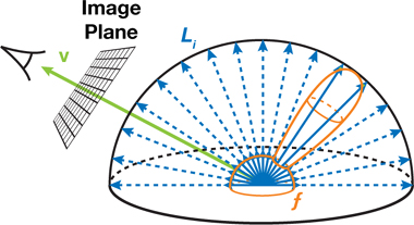
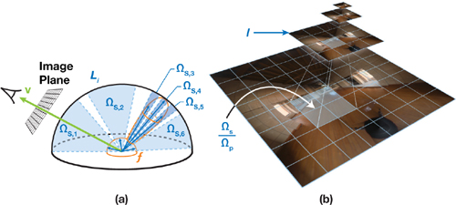
The goal in rendering is to compute, for each pixel, how much light from the surrounding environment is reflected toward the virtual camera at a given surface point, as shown in Figure 20-2. To convert the incoming light from one particular direction, Li(u), into reflected light toward the direction of the camera, v, we use the material function f, known as the bidirectional reflectance distribution function (BRDF). One common BRDF is the classic Phong reflection model. To compute the total reflected light, Lo(v), the contributions from every incident direction, u, must be summed (or integrated, in the limit) together over the hemisphere H:
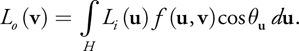
This equation is referred to as the reflectance equation or the illumination integral. Here, θu is the angle between the surface normal and the incoming light’s direction u.
In image-based lighting, the incoming light Li is approximated by an environment map, where each texel corresponds to an incoming direction u and occlusion is ignored. However, even with this approximation, the numerical integration of the illumination integral for one pixel in the image requires thousands of texels in the environment map to be multiplied with the BRDF and summed. This operation is clearly too computationally expensive for real-time rendering.
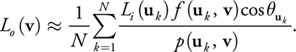
We cannot afford evaluating the illumination integral for all incident directions, so we randomly choose a number of directions and evaluate the integrated function, Li(u)f (u, v)cos θu, at these directions to obtain samples, or estimates of the integral. The average of these samples produces an approximation of the integral, which is the essence of Monte Carlo quadrature. In fact, if we had an infinite set of samples, the average of the samples would equal the true value of the integral. However, when we use only a practical, finite set of samples, the average value varies from the actual solution and introduces noise into the image, as shown in Figure 20-5b (in Section 20.4). One way to reduce this noise is to choose the most important samples that best approximate the integral.
Generating uniform random directions is not the best method for approximating the integral if we have a rough idea about the behavior of the integrated function. For instance, if we are integrating a glossy material with the environment, it makes the most sense to sample directions around the specular direction (in other words, the mirror reflection direction), because much of the reflected light originates from these directions. To represent this mathematically, a probability density function (PDF) is used to define the optimal directions for sampling. The PDF is a normalized function, where the integral over the entire domain of the function is 1 and the peaks represent important regions for sampling.
However, when we skew sample directions, not all estimates of the integral are equal, and thus we must weight them accordingly when averaging all the samples. For instance, one sample in a low-value region of the PDF is representative of what would be many samples if uniform sampling were used. Similarly, one sample in a high-value PDF region represents only a few samples with uniform sampling. To compensate for this property of the PDF-proportional sampling, we multiply each sample by the inverse of the PDF. This yields a Monte Carlo estimator that uses the weighted average of all the samples:
To define the optimal PDF for the illumination integral, we need an accurate approximation of the product between the material BRDF and the incident lighting. However, generating samples according to this product is quite involved (Clarberg et al. 2005). Fortunately, creating samples according to the BRDF alone is straightforward, and when we use it in combination with sample filtering—described in Section 20.1.4—it provides good results.
Because BRDFs are a part of the integration, they serve as a good measure to guide the sampling to produce directions that best approximate the integral. Here, we use a normalized BRDF as the PDF for sampling. To sample this PDF, we convert a random number pair into an important direction for the BRDF. For example, Equations 7 and 8, later in this section, perform such a conversion for the specular lobe of the Phong BRDF. If you are interested in how such sampling formulas are derived, keep reading.
We find the sample directions by converting the PDF into a cumulative distribution function (CDF). Intuitively, think of a CDF as a mapping between a PDF-proportional distribution and a uniform distribution. In the discrete case, where there are only a finite number of samples, we can define the CDF by stacking each sample. For instance, if we divide all possible sampling directions for rendering into four discrete directions, where one of the sample directions, S2, is known a priori to be more important, then the probabilities of the four samples can be stacked together as depicted in Figure 20-3.
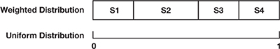
In this case, if we choose a random number, where there exists an equal likelihood that any value between 0 and 1 will be produced, then more numbers will map to the important sample, S2, and thus we will sample that direction more often.
For continuous one-dimensional PDFs, we must map an infinite number of the PDF weighted samples to a uniform distribution of numbers. This way, we can generate a random number from a uniform distribution and be more likely to obtain an important sample direction, just as more random values would map to the important sample S2. The mapping is performed by the same stacking operation, which is represented as the integral of the infinite sample directions. We can obtain the position of a sample s within the uniform distribution by stacking all the previous weighted samples, p(θ) dθ, before s on top of each other via integration:
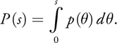
To obtain the PDF-proportional sample from a random number, we set P(s) equal to a random value ξ and solve for s. In general, we denote the mapping from the random value to the sample direction distributed according to the PDF as P-1(ξ).
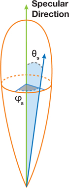
As an example, let us sample the glossy component of the Phong BRDF (Lewis 1994). The glossy component assumes light is reflected based upon a cosine falloff from the specular reflection direction computed as the mirror reflection of the viewing direction v with respect to the normal of the surface. We can represent the glossy component mathematically as cosnθs, where θs is the angle between the sample direction and the specular direction, and n is the shininess of the surface. To convert this material function into a PDF, p(θs, φs), we must first normalize the cosine lobe to integrate to one:
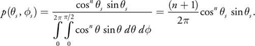
Here, θs and φs are the spherical coordinates of the sample direction in a coordinate frame where the specular direction is the z-axis, as shown in Figure 20-4. The extra sine appears because we work with spherical coordinates instead of the intrinsic parameterization of directions by differential solid angles.
To generate the two-dimensional importance sample direction (θs, φs) according to this PDF, it is best if we find each dimension of the sample direction separately. Therefore, we need a PDF for each dimension so we can apply Equation 3 to convert the PDF into a CDF and create a partial sample direction. To accomplish this, the marginal probability of the θs direction, p(θs), can be separated from p(θs, φs) by integrating the PDF across the entire domain of φs:
This one-dimensional PDF can now be used to generate θs. Given the value of θs, we find the PDF for φs using the conditional probability p(φs |θs) defined as
The two probability functions are converted into CDFs by Equation 3 and inverted to map a pair of independent uniform random variables (ξ1, ξ2) to a sample direction (θs,φs)[1]:
To operate in a Cartesian space, the spherical coordinates are simply mapped to their Cartesian counterparts:

Remember, xs, ys, and zs are defined in a coordinate frame where the specular direction is the z-axis (see Figure 20-4). To sample the surrounding environment, the sample direction must be transformed to world space. This rotation is done by applying two linear transformations: tangent-space to world-space and specular-space to tangent-space. Tangent-space to world-space is derived from the local tangent, binormal, and normal at the surface point. The specular-space to tangent-space transformation is underconstrained because only the specular direction defines the space. Thus, we introduce an arbitrary axis-aligned vector to generate the transformation.
Similar importance sampling methods can be used for other material models, such as the Lafortune BRDF (Lafortune et al. 1997) or Ward’s anisotropic BRDF (Walter 2005). Pharr and Humphreys 2004 gives more details on deriving sampling formulas for various BRDFs.
The problem with generating random sample directions using pseudorandom numbers is that the directions are not well distributed, which leads to poor accuracy of the estimator in Equation 2. We can improve accuracy by replacing pseudorandom numbers with quasirandom low-discrepancy sequences, which intrinsically guarantee well-distributed directions. One such sequence is known as the Hammersley sequence. A random pair xi in the two-dimensional Hammersley sequence with N values is defined as
where the radical inverse function, φ2(i) returns the number obtained by reflecting the digits of the binary representation of i around the decimal point, as illustrated in Table 20-1.
Another problem, pertaining both to pseudorandom numbers and the low-discrepancy series, is that it is computationally expensive to generate random sample directions on the GPU. Instead, we precompute the numbers on the CPU and store them as literals in the shader or upload them into the constant registers to optimize the algorithm. As a consequence, the same sequence of quasirandom numbers is used for integration when computing the color of each pixel. The use of such deterministic number sequences, in combination with a relatively low sample count, produces an aliasing effect, as shown in Figure 20-5a, that we suppress by filtering the samples, as detailed in the next section.
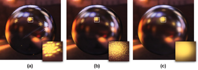
As shown in Figure 20-5a, deterministic importance sampling causes sharp aliasing artifacts that look like duplicate specular reflections. In standard Monte Carlo quadrature, this problem is combated by introducing randomness, which changes aliasing into more visually acceptable noise, as is evident in Figure 20-5b. However, keeping the noise level low requires using hundreds or even thousands of samples for each pixel—which is clearly not suitable for real-time rendering on the GPU. We use a different approach—filtering with mipmaps—to reduce aliasing caused by the low sample count, as shown in Figure 20-5c.
The idea is as follows: if the PDF of a sample direction is small (that is, if the sample is not very probable), it is unlikely that other samples will be generated in a similar direction. In such a case, we want the sample to bring illumination from the environment map averaged over a large area, thereby providing a better approximation of the overall integration. On the other hand, if the PDF of a direction is very high, many samples are likely to be generated in similar directions. Thus, multiple samples will help average out the error in the integral estimation from this region. In this case, the sample should only average a small area of the environment map, as shown in Figure 20-6a.
(a) Various samples and their associated solid angle Ωs, as defined in Equation 12, for the illumination integral. (b) A visualization of a mipmapped environment texture, where Ωs/Ωp is shown on the zeroth level of the environment map and the corresponding filtered sample is highlighted on level l.
Figure 20-6. Illustration of Filtered Importance Sampling
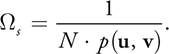
In short, the lower the PDF, the more pixels of the environment should be averaged for that sample. We define this relationship in terms of the solid angle associated with a sample, computed as the inverse of the product between the PDF and the total number of samples, N:
Here, we should average all pixels of the environment map within the solid angle Ωs around a sample direction. To make the averaging efficient, we use the mipmap data structure available on the GPU. Remember, the mipmap is a pyramidal structure over a texture, where each pixel of level l is the average of the four corresponding pixels of level l– 1, as shown in Figure 20-6b, and level zero is the original texture. Therefore, averaging all the pixels within the solid angle Ωs can be approximated by choosing an appropriate level of the mipmap.
Here is how we proceed. First, we need to compute the number of environment map pixels in Ωs. This number is given by the ratio of Ωs to the solid angle subtended by one pixel of the zeroth mipmap level Ωp, which in turn, is given by the texture resolution, w · h, and the mapping distortion factor d(u):
Let us assume for a while that the distortion d(u) is known (we will get back to it in Section 20.4.1).
As a reminder, we want the environment map lookup to correspond to averaging ΩsΩppixels, which yields a simple formula for the mipmap level:
Notice that all solid angles are gone from the final formula! In addition, the ![]() log2[(w · h)/N] expression can be precomputed with minimal computational cost. Now all we need to do for each sample direction is to evaluate the PDF p(u, v) and the distortion d(u), plug these numbers into the preceding formula, and feed the result to
log2[(w · h)/N] expression can be precomputed with minimal computational cost. Now all we need to do for each sample direction is to evaluate the PDF p(u, v) and the distortion d(u), plug these numbers into the preceding formula, and feed the result to tex2Dlod() as the level-of-detail (LOD) parameter when we look up the environment map.
In practice, we found that introducing small amounts of overlap between samples (for example, biasing ΩsΩp by a constant) produces smoother, more visually acceptable results. Specifically, we perform the bias by adding 1 to the calculated mipmap level defined by Equation 13.
Cube maps are typically used for environment mapping. However, although cube maps have very low distortion (which is good), they also have a serious flaw—the mipmap generation is performed on each face separately. Unfortunately, our filtering operation assumes that the mipmap is generated by averaging pixels from the entire environment map. Therefore, we need a way to introduce as much surrounding information of the environment map as possible into a single image, which will reduce seamlike artifacts from the mipmaps without modifying the hardware-accelerated mipmap generation.
Thus, instead of using cube maps, we use dual-paraboloid environment maps (Heidrich and Seidel 1998, Kilgard 1999). The environment is stored in two textures: one represents directions from the upper hemisphere (z≥ 0) and the other represents directions from the lower hemisphere (z < 0). Although the mipmap for the two textures is computed separately, artifacts rarely appear in rendered images. Why? Because the texture corresponding to each hemisphere contains some information from the opposite hemisphere.
Still, some occasional seams in the rendered images might correspond to the sampling from the environment map at a location where the circle in Figure 20-7a touches the edge of the texture. To remedy this situation, we adjust the usual paraboloid mapping by adding a scaling factor b of 1.2, which adds even more information from the opposite hemisphere, as shown in Figure 20-7b.
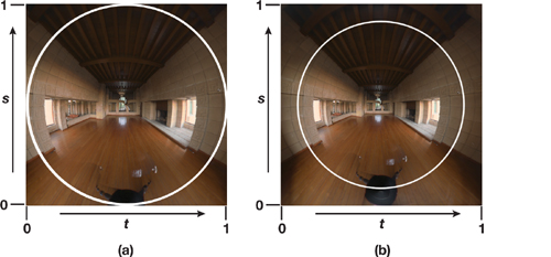
(a) The texture corresponding to a hemisphere in dual-paraboloid mapping contains some information from the opposite hemisphere (the region outside the circle). (b) Scaling the (s, t) texture coordinates introduces even more information from the opposite hemisphere.
Figure 20-7. Scaled Dual-Paraboloid Environment Mapping
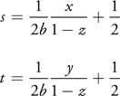
Given a direction, u = (x, y, z), the (s, t) texture coordinates for this scaled mapping are computed as follows in Table 20-2.

By computing the inverse of the Jacobian determinant of this mapping, we can model the rate of change from a unit of area on the hemisphere to a unit of area on the texture (in other words, the distortion for the mapping, d(u)):
As seen in Listing 20-1, the implementation of the algorithm follows straight from the Monte Carlo estimator (Equation 2) and the computation of the mipmap level (Equation 13). To optimize image quality and performance, we use a spherical harmonics representation for the diffuse component of the material (Ramamoorthi 2001). Spherical harmonics work well for low-frequency diffuse shading and, together with our sampling approach for glossy shading, provide an ideal hybrid solution.
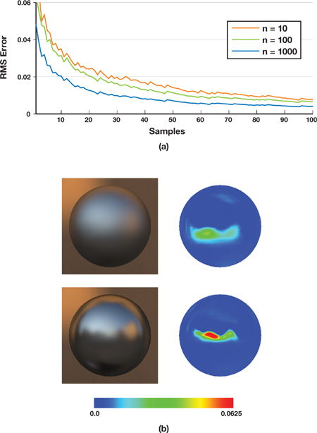
Figure 20-8a plots the error of the approximation with respect to a reference solution, demonstrating that the fidelity of the rendering directly correlates to the number of samples used. In practice, only 24 or fewer samples are needed for surfaces with complex geometry. Smooth surfaces, such as the spheres in Figure 20-8b, often need more samples, but 40 samples are sufficient for visually acceptable solutions. Thus, much like the wavelet-based approaches, the filtered importance sampling does not require many samples to produce accurate, glossy surface reflection. In addition, Figure 20-9 shows that our technique performs well on a variety of GPUs and that the performance varies almost linearly with the number of samples.

Example 20-1. Pseudocode for Our Sampling Algorithm
The actual implementation of the shader looks slightly different from this pseudocode, but it is indeed just an optimized version. The most important optimizations are these: (1) Four directions are generated in parallel. (2) The BRDF is not explicitly evaluated, because it only appears divided by the PDF, which cancels out most of the terms of the BRDF. (3) The trigonometric functions associated with generating a sample direction using the Hammersley sequence (Equation 10) are precomputed.
float4 GPUImportanceSampling(
  float3 viewing : TEXCOORD1
  uniform sampler2D env) : COLOR
{
  float4 c = 0;

  // Sample loop
  for (int k=0; k < N; k++) {
    float2 xi = hammersley_seq(k);
    float3 u = sample_material(xi);
    float pdf = p(u, viewing);
    float lod = compute_lod(u, pdf);
    float3 L = tex2Dlod(env, float4(texcoord, lod.xy));
    c += L*f(u,viewing)/pdf;
  }

  return c/N;
}Our GPU-based importance sampling is a real-time rendering algorithm for various parameterized material models illuminated by an environment map. Performing Monte Carlo integration with mipmap-based filtering sufficiently reduces the computational complexity associated with importance sampling to a process executable within a single GPU shader. This combination also shows that non-BRDF-specific filters (such as mipmaps) are sufficient for approximating the illumination integral. Consequently, BRDFs and environments can be changed in real time.
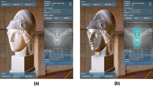
Given that the BRDF and environment can be completely dynamic, visualizations for applications such as material or lighting design become trivial and afford new user interfaces. In Figure 20-10, we show such an interface for a spatially varying BRDF painting program, in which the user can choose a parameterization of a BRDF and paint it onto the mesh in real time. In general, our technique provides a rendering solution that is easy to integrate into existing production pipelines by using a single shader that harnesses the computational power of the GPU.
For a more in-depth introduction into Monte Carlo and its uses in rendering, we suggest reading Physically Based Rendering: From Theory to Implementation (Pharr and Humphreys 2004). Additionally, Alexander Keller’s report, “Strictly Deterministic Sampling Methods in Computer Graphics” (Keller 2003), provides detailed information on using quasirandom low-discrepancy sequences and other random number sequences for rendering.
[1] The integration for p(θs) is actually (1–ξ1)1/(n+1), but because ξ1 is a uniformly distributed random variable between 0 and 1, (1–ξ1) is also uniformly distributed between 0 and 1.