We present an incremental method for computing the Gaussian at a sequence of regularly spaced points, with the cost of one vector multiplication per point. This technique can be used to implement image blurring by generating the Gaussian coefficients on the fly, avoiding an extra texture lookup into a table of precomputed coefficients.
Filtering is a common operation performed on images and other kinds of data in order to smooth results or attenuate noise. Usually the filtering is linear and can be expressed as a convolution:
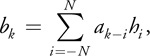
where ai is an input sequence, bi is an output sequence, and hi is the kernel of the convolution.
One of the most popular filtering kernels is the Gaussian:
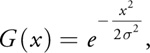
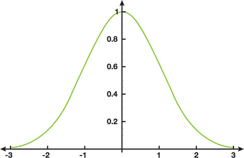
where σ is a parameter that controls its width. Figure 40-1 shows a graph of this function for σ = 1.
When used for images in 2D, this function is both separable and radially symmetric:
We can take advantage of this symmetry to considerably reduce the complexity of the computations.
Gaussian blurring has a lot of uses in computer graphics, image processing, and computer vision, and the performance can be enhanced by utilizing a GPU, because the GPU is well suited to image processing (Jargstorff 2004). The fragment shader for such a computation is shown in Listing 40-1.
In Listing 40-1,acc implements the summation in Equation 1, coeff is one of the coefficients hi in the kernel of the convolution, texture2D() is the input sequence ak–i, and gl_FragColor is one element of the output sequence bk.
The coefficient computations involve some relatively expensive operations (an exponential and a division), as well as some cheaper multiplications. The expensive operations can dominate the computation time in the inner loop. An experienced practitioner can reduce the coefficient computations to
coeff = exp(-u * u);but still, there is the exponential computation on every pixel.
One approach to overcome these expensive computations would be to precompute the coefficients and look them up in a texture. However, there are already two other texture fetches in the inner loop, and we would prefer to do some computations while waiting for the memory requests to be fulfilled.
Example 40-1.
uniform sampler2D inImg;  // source image
uniform float     sigma;  // Gaussian sigma
uniform float     norm;   // normalization, e.g. 1/(sqrt(2*PI)*sigma)
uniform vec2      dir;    // horiz=(1.0, 0.0), vert=(0.0, 1.0)
uniform int       support; // int(sigma * 3.0) truncation
void main()
{
  vec2 loc = gl_FragCoord.xy;    // center pixel cooordinate
  vec4 acc;                      // accumulator
  acc = texture2D(inImg, loc);   // accumulate center pixel
  for (i = 1; i <= support; i++) {
    float coeff = exp(-0.5 * float(i) * float(i) / (sigma * sigma));
    acc += (texture2D(inImg, loc - float(i) * dir)) * coeff; // L
    acc += (texture2D(inImg, loc + float(i) * dir)) * coeff; // R
  }
  acc *= norm;            // normalize for unity gain
  gl_fragColor = acc;
}
Another approach would be to compute the Gaussian using one of several polynomial or rational polynomial approximations that are chosen based on the range of the argument. However, range comparisons are inefficient on a GPU, and the table of polynomial coefficients would most likely need to be stored in a texture, so this is less advantageous than the previous approach.
Our approach is to compute the coefficients on the fly, taking advantage of the coherence between adjacent samples to perform the computations incrementally with a small number of simple instructions. The technique is analogous to polynomial forward differencing, so we take a moment to describe that technique first.
Suppose we wish to evaluate a polynomial
M times at regular intervals δ starting at t0, that is,
{t0, t0 + δ + 2δ, ..., t0 + (M-1)δ}. |
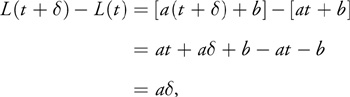
We hope to use the coherence between successive values to decrease the amount of computation at each point. We know that, for a linear (that is, second order) polynomial L(t) = at + b, the difference between successive values is constant:
which results in the following forward-differencing algorithm to compute a sequence of linear function values at regular intervals dt, starting at a point t0:
p0 = a * t0 + b;
p1 = a * dt;
for (i = 0; i < LENGTH; i++) {
  DoSomethingWithTheFunctionValue(p0);
  p0 += p1;
}
We extend this algorithm to an N-order polynomial by taking higher-order differences and maintaining them in N variables whose values at iteration i are denoted as
These N variables are initialized as the repeated differences of the polynomial evaluated at successive points:
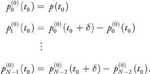
That is, we first take differences of the polynomial evaluated at regular intervals, and then we take differences of those differences, and so on. It should come as no surprise that the Nth difference is zero for an Nth-order polynomial, because the differences are related to derivatives, and the Nth derivative of an Nth-order polynomial is zero. Moreover, the (N - 1)th difference (and derivative) is constant.
At each iteration i, the N state variables are updated by incrementing ![]()
The value of the polynomial at t0 + iδ is then given by ![]() .
.
For example, to incrementally generate a cubic polynomial
we initialize the forward differences as such:
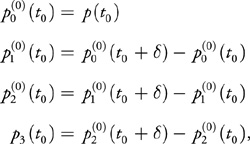
where ![]() is the value of the polynomial at the initial point,
is the value of the polynomial at the initial point, ![]() and
and ![]() are the first and second differences at the initial point, and p3 is the constant second difference. Note that we have dropped the iteration superscript on p3 because it is constant.
are the first and second differences at the initial point, and p3 is the constant second difference. Note that we have dropped the iteration superscript on p3 because it is constant.
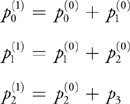
To evaluate the polynomial at t0 + δ by the method of forward differences, we increment p0 by p1, p1 by p2, and p2 by p3:
and the value is given by ![]() .
.
Similarly, the value of the polynomial at t0 + 2δ is computed from the previous forward differences:
and so on. Note that in the case of a cubic polynomial, we can use a single state vector to store the forward differences. Utilizing the powerful expressive capabilities of GLSL, we can implement the state update in one instruction:
p.xyz += p.yzw;
where we have initialized the forward-difference vector as follows:
p = f(vec4(t, t+d, t+2*d, t+3*d));
p.yzw -= p.xyz;
p.zw  -= p.yz;
p.w   -= p.z;
Note that this method can be used to compute arbitrary functions, not just polynomials. Forward-differencing is especially useful for rendering in 2D and 3D graphics using scan-conversion techniques for lines and polygons (Foley et al. 1990). Adaptive forward differencing was developed in a series of papers (Lien et al. 1987, Shantz and Chang 1988, and Chang et al. 1989) for evaluating and shading cubic and NURBS curves and surfaces in floating-point and fixed-point arithmetic. Klassen (1991a) uses adaptive forward differencing to draw antialiased cubic spline curves. Turkowski (2002) renders cubic and spherical panoramas in real time using forward differencing of piecewise polynomials adaptively approximating transcendental functions.
Our initialization method corresponds to the Taylor series approximation. More accurate approximations over the desired domain can be achieved by using other methods of polynomial approximation, such as Lagrangian interpolation or Chebyshev approximation (Ralston and Rabinowitz 1978).
When we apply the forward-differencing technique to the Gaussian, we get poor results, as shown in Figure 40-2.
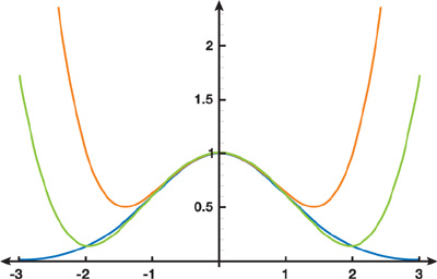
The orange curve in Figure 40-2 is the Taylor series approximation at 0, and the green curve is a polynomial fit to the points {0.0, 1.0, 2.0}. The black curve is the Gaussian. The fundamental problem is that polynomials get larger when their arguments do, whereas the Gaussian gets smaller.
The typical numerical analysis approach is to instead use a rational polynomial of the form
We can also use forward differencing to compute the numerator and the denominator separately, but we still have to divide them at each pixel. This algorithm does indeed produce a better approximation and has the desired asymptotic behavior. This is a good technique for approximating a wide class of functions, but we can take advantage of the exponential nature of the Gaussian to yield a method that is simpler and faster. It turns out that we have such an algorithm that shares the simplicity of forward differencing if we replace differences by quotients.
Given the Gaussian
we evaluate the quotient of successive values
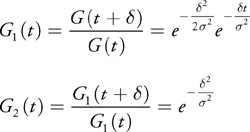
and we find that the second quotient is constant, whereas the first quotient is exponential, as illustrated in Figure 40-3.
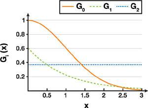
The next quotient would yield another constant: 1. These properties have a nice analogy to those of forward differencing, where quotients take the place of differences, and a quotient of 1 takes the place of a difference of 0.
Note that there are two factors in the first quotient: one is related purely to the sampling spacing δ, and the other is an attenuation from t = 0. In fact, when we set t = 0, we get
Only one exponential evaluation is needed to generate any number of regularly spaced samples starting at zero. The entire Gaussian is characterized by one attenuation factor, as shown in Listing 40-2.
Example 40-2.
#ifdef USE_SCALAR_INSTRUCTIONS // suitable for scalar GPUs

float g0, g1, g2;
g0 = 1.0 / (sqrt(2.0 * PI) * sigma);
g1 = exp(-0.5 * delta * delta / (sigma * sigma));
g2 = g1 * g1;

for (i = 0; i < N; i++) {
  MultiplySomethingByTheGaussianCoefficient(g0);
  g0 *= g1;
  g1 *= g2;
}
#else // especially for vector architectures

float3 g;
g.x = 1.0 / (sqrt(2.0 * PI) * sigma);
g.y = exp(-0.5 * delta * delta / (sigma * sigma));
g.z = g.y * g.y;

for (i = 0; i < N; i++) {
  MultiplySomethingByTheGaussianCoefficient(g.x);
  g.xy *= g.yz;
}
#endif // USE_VECTOR_INSTRUCTIONS
The Gaussian coefficients are generated with just one vector multiplication per sample. A vector multiplication is one of the fastest instructions on the GPU.
The incremental Gaussian algorithm is exact with exact arithmetic. In this section, we perform a worst-case error analysis, taking into account (1) errors in the initial coefficient values, which are due to representation in single-precision IEEE floating-point (that is, a(1 + ε)) and (2) error that is due to floating-point multiplication (ab(1 + ε)). Then we determine how the error grows with each iteration.
Let the initial relative error of any of the forward quotient coefficients be a stochastic variable ε so that its floating-point representation is
instead of a, because it is approximated in a finite floating-point representation. For single-precision IEEE floating-point, for example,
The product of two finite-precision numbers c and d is
instead of cd because the product will be truncated to the word length. Putting this together, we find that the relative error of the product of two approximate variables a and b is
Thus, the errors accumulate. As is traditional with error analysis, we drop the higherorder terms in ε, because they are much less significant.
The relative error for the coefficients is shown in Table 40-1, computed simply by executing the incremental Gaussian algorithm with the error accumulation just given. Here, we do two exponential computations: one for the first-order quotient g1 and one for the second-order quotient g2, to maximize the precision.
The error in g1 increases linearly, because it is incremented by the constant g2 every iteration. The error in g0 also accumulates the error in g1, so it grows quadratically. The error for g0 can then be expressed as a polynomial function of n:
If the initial error ε is 1/2 of the least significant bit of a single-precision floating-point number and we wish the coefficients to have a relative error of 1/256, then the parenthesized quantity in the Equation 18 should be less than 217. This suggests n ≤ 361.
Typically, however, practitioners truncate the Gaussian at 3σ, where
The error in the last evaluation (at 3σ), relative to the central coefficient is still only
when we compute it with 361 forward products. If we are willing to have a maximum error of 1/256 relative to the central coefficient (as opposed to the error relative to the fringe coefficient), then we can go up to 3,435 samples. When these coefficients are used to implement a convolution kernel, this is the kind of accuracy that we need.
We have a different situation if we choose to do only one exponential computation for the first quotient and compute the second difference from the first. In this case the error in the second quotient is doubled, as shown in Table 40-2.
The error for g0 in this scenario is
with the maximum number of iterations for 8-bit accuracy 295 or 2,804, depending on whether the relative accuracy desired is relative to the fringe or the central coefficients, respectively.
For image-blurring applications, the fringe error relative to the central coefficient is of primary concern. Even when we compute g2 from g1, the limitation of 3σ ≤ 2804, or σ ≤ 934 is not restrictive (because applications with σ > 100 are rare), so it suffices to compute only the g1 coefficient as an exponential, and g2 as its square.
Processor performance has increased substantially over the past decade, so that arithmetic logic unit (ALU) operations are executed faster than accessing memory, by one to three orders of magnitude. As a result, algorithms on modern computer architectures benefit from replacing table lookups with relatively simple computations, especially when the tables are relatively large.
The incremental computation algorithm is noticeably faster on the GPU and CPU than looking up coefficients in a table. While GPU performance highly depends on the capabilities of the hardware, the GPU vendor, the driver version, and the operating system version, we can conservatively say that the technique yields at least a 15 percent performance improvement.
Another aspect of performance is whether a particular blur filter can fit on the GPU. The incremental Gaussian blur algorithm may appear to be small, but the GPU driver will increase the number of instructions dramatically, under certain circumstances. In particular, some GPUs do not have any looping primitives, so the driver will automatically unroll the loop. The maximum loop size (that is, the Gaussian radius) is then limited by the number of ALU instructions or texture lookup instructions. This algorithm will then reduce the number of texture lookups to increase the maximum blur radius.
Graphics hardware architecture is constantly evolving. While texture access is relatively slow compared to arithmetic computations, some newer hardware (such as the GeForce 8800 Series) incorporates up to 16 constant buffers of 16K floats each, with the same access time as a register. The incremental Gaussian algorithm may not yield any higher performance than table lookup using such constant buffers, but it may not yield lower performance either. The incremental Gaussian algorithm has the advantage that it can be deployed successfully on a wide variety of platforms.
We have presented a very simple technique to evaluate the Gaussian at regularly spaced points. It is not an approximation, and it has the simplicity of polynomial forward differencing, so that only one vector instruction is needed for a coefficient update at each point on a GPU.
The method of forward quotients can accelerate the computation of any function that is the exponential of a polynomial. Modern computers can perform multiplications as fast as additions, so the technique is as powerful as forward differencing. This method opens up incremental computations to a new class of functions.
I would like to thank Nathan Carr for encouraging me to write a chapter on this algorithm, and Paul McJones for suggesting a contribution to GPU Gems. Gavin Miller, Frank Jargstorff and Andreea Berfield provided valuable feedback for improving this paper. I would like to thank Frank Jargstorff for his evaluation of performance on the GPU.