
Chapter 3. Variational Autoencoders
In 2013, Diederik P. Kingma and Max Welling published a paper that laid the foundations for a type of neural network known as a variational autoencoder (VAE).1 This is now one of the most fundamental and well-known deep learning architectures for generative modeling. In this chapter, we shall start by building a standard autoencoder and then see how we can extend this framework to develop a variational autoencoder—our first example of a generative deep learning model.
Along the way, we will pick apart both types of model, to understand how they work at a granular level. By the end of the chapter you should have a complete understanding of how to build and manipulate autoencoder-based models and, in particular, how to build a variational autoencoder from scratch to generate images based on your own training set.
Let’s start by paying a visit to a strange art exhibition…
The Art Exhibition
Two brothers, Mr. N. Coder and Mr. D. Coder, run an art gallery. One weekend, they host an exhibition focused on monochrome studies of single-digit numbers. The exhibition is particularly strange because it contains only one wall and no physical artwork. When a new painting arrives for display, Mr. N. Coder simply chooses a point on the wall to represent the painting, places a marker at this point, then throws the original artwork away. When a customer requests to see the painting, Mr. D. Coder attempts to re-create the artwork using just the coordinates of the relevant marker on the wall.
The exhibition wall is shown in Figure 3-1, where each black dot is a marker placed by Mr. N. Coder to represent a painting. We also show one of the paintings that has been marked on the wall at the point [–3.5, –0.5] by Mr. N. Coder and then reconstructed using just these two numbers by Mr. D. Coder.

Figure 3-1. The wall at the art exhibition
In Figure 3-2 you can see examples of other original paintings (top row), the coordinates of the point on the wall given by Mr. N. Coder, and the reconstructed paintings produced by Mr. D. Coder (bottom row).

Figure 3-2. More examples of reconstructed paintings
So how does Mr. N. Coder decide where to place the markers? The system evolves naturally through years of training and working together, gradually tweaking the processes for marker placement and reconstruction. The brothers carefully monitor the loss of revenue at the ticket office caused by customers asking for money back because of badly reconstructed paintings, and are constantly trying to find a system that minimizes this loss of earnings. As you can see from Figure 3-2, it works remarkably well—customers who come to view the artwork very rarely complain that Mr. D. Coder’s re-created paintings are significantly different from the original pieces they came to see.
One day, Mr. N. Coder has an idea. What if he randomly placed markers on parts of the wall that currently do not have a marker? Mr. D. Coder could then re-create the artwork corresponding to these points, and within a few days they would have their own exhibition of completely original, generated paintings.
The brothers set about their plan and open their new exhibition to the public. Some of the exhibits and corresponding markers are displayed in Figure 3-3.

Figure 3-3. The new generative art exhibition
As you can see, the plan was not a great success. The overall variety is poor and some pieces of artwork do not really resemble single-digit numbers.
So, what went wrong and how can the brothers improve their scheme?
Autoencoders
The preceding story is an analogy for an autoencoder, which is a neural network made up of two parts:
-
An encoder network that compresses high-dimensional input data into a lower-dimensional representation vector
-
A decoder network that decompresses a given representation vector back to the original domain
This process is shown in Figure 3-4.

Figure 3-4. Diagram of an autoencoder
The network is trained to find weights for the encoder and decoder that minimize the loss between the original input and the reconstruction of the input after it has passed through the encoder and decoder.
The representation vector is a compression of the original image into a lower-dimensional, latent space. The idea is that by choosing any point in the latent space, we should be able to generate novel images by passing this point through the decoder, since the decoder has learned how to convert points in the latent space into viable images.
In our analogy, Mr. N. Coder and Mr. D. Coder are using representation vectors inside a two-dimensional latent space (the wall) to encode each image. This helps us to visualize the latent space, since we can easily plot points in 2D. In practice, autoencoders usually have more than two dimensions in order to have more freedom to capture greater nuance in the images.
Autoencoders can also be used to clean noisy images, since the encoder learns that it is not useful to capture the position of the random noise inside the latent space. For tasks such as this, a 2D latent space is probably too small to encode sufficient relevant information from the input. However, as we shall see, increasing the dimensionality of the latent space quickly leads to problems if we want to use the autoencoder as a generative model.
Your First Autoencoder
Let’s now build an autoencoder in Keras. This example follows the Jupyter notebook 03_01_autoencoder_train.ipynb in the book repository.
Generally speaking, it is a good idea to create a class for your model in a separate file. This way, you can instantiate an Autoencoder object with parameters that define a particular model architecture in the notebook, as shown in Example 3-1. This makes your model very flexible and able to be easily tested and ported to other projects as necessary.
Example 3-1. Defining the autoencoder
frommodels.AEimportAutoencoderAE=Autoencoder(input_dim=(28,28,1),encoder_conv_filters=[32,64,64,64],encoder_conv_kernel_size=[3,3,3,3],encoder_conv_strides=[1,2,2,1],decoder_conv_t_filters=[64,64,32,1],decoder_conv_t_kernel_size=[3,3,3,3],decoder_conv_t_strides=[1,2,2,1],z_dim=2)
Let’s now take a look at the architecture of an autoencoder in more detail, starting with the encoder.
The Encoder
In an autoencoder, the encoder’s job is to take the input image and map it to a point in the latent space. The architecture of the encoder we will be building is shown in Figure 3-5.

Figure 3-5. Architecture of the encoder
To achieve this, we first create an input layer for the image and pass this through four Conv2D layers in sequence, each capturing increasingly high-level features. We use a stride of 2 on some of the layers to reduce the size of the output. The last convolutional layer is then flattened and connected to a Dense layer of size 2, which represents our two-dimensional latent space.
Example 3-2 shows how to build this in Keras.
Example 3-2. The encoder
### THE ENCODERencoder_input=Input(shape=self.input_dim,name='encoder_input')x=encoder_inputforiinrange(self.n_layers_encoder):conv_layer=Conv2D(filters=self.encoder_conv_filters[i],kernel_size=self.encoder_conv_kernel_size[i],strides=self.encoder_conv_strides[i],padding='same',name='encoder_conv_'+str(i))x=conv_layer(x)x=LeakyReLU()(x)shape_before_flattening=K.int_shape(x)[1:]x=Flatten()(x)encoder_output=Dense(self.z_dim,name='encoder_output')(x)self.encoder=Model(encoder_input,encoder_output)

Define the input to the encoder (the image).

Stack convolutional layers sequentially on top of each other.

Flatten the last convolutional layer to a vector.

Denselayer that connects this vector to the 2D latent space.
The Keras model that defines the encoder—a model that takes an input image and encodes it into the 2D latent space.
You can change the number of convolutional layers in the encoder simply by adding elements to the lists that define the model architecture in the notebook. I strongly recommend experimenting with the parameters that define the models in this book, to understand how the architecture affects the number of weights in each layer, model performance, and model runtime.
The Decoder
The decoder is a mirror image of the encoder, except instead of convolutional layers, we use convolutional transpose layers, as shown in Figure 3-6.
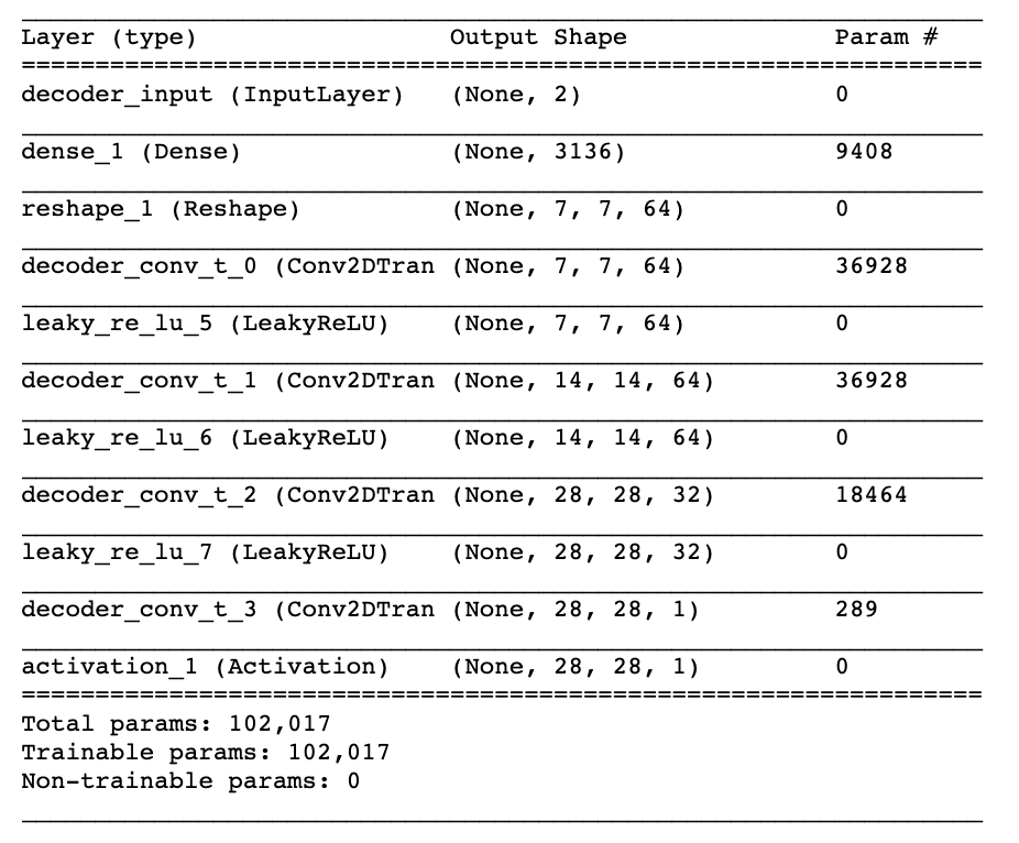
Figure 3-6. Architecture of the decoder
Note that the decoder doesn’t have to be a mirror image of the encoder. It can be anything you want, as long as the output from the last layer of the decoder is the same size as the input to the encoder (since our loss function will be comparing these pixelwise).
Example 3-3 shows how we build the decoder in Keras.
Example 3-3. The decoder
### THE DECODERdecoder_input=Input(shape=(self.z_dim,),name='decoder_input')x=Dense(np.prod(shape_before_flattening))(decoder_input)x=Reshape(shape_before_flattening)(x)foriinrange(self.n_layers_decoder):conv_t_layer=Conv2DTranspose(filters=self.decoder_conv_t_filters[i],kernel_size=self.decoder_conv_t_kernel_size[i],strides=self.decoder_conv_t_strides[i],padding='same',name='decoder_conv_t_'+str(i))x=conv_t_layer(x)ifi<self.n_layers_decoder-1:x=LeakyReLU()(x)else:x=Activation('sigmoid')(x)decoder_output=xself.decoder=Model(decoder_input,decoder_output)
Define the input to the decoder (the point in the latent space).
Connect the input to a
Denselayer.Reshape this vector into a tensor that can be fed as input into the first convolutional transpose layer.
Stack convolutional transpose layers on top of each other.
The Keras model that defines the decoder—a model that takes a point in the latent space and decodes it into the original image domain.
Joining the Encoder to the Decoder
To train the encoder and decoder simultaneously, we need to define a model that will represent the flow of an image through the encoder and back out through the decoder. Luckily, Keras makes it extremely easy to do this, as you can see in Example 3-4.
Example 3-4. The full autoencoder
### THE FULL AUTOENCODERmodel_input=encoder_input#model_output=decoder(encoder_output)#self.model=Model(model_input,model_output)#
The input to the autoencoder is the same as the input to the encoder.
The output from the autoencoder is the output from the encoder passed through the decoder.
The Keras model that defines the full autoencoder—a model that takes an image, and passes it through the encoder and back out through the decoder to generate a reconstruction of the original image.
Now that we’ve defined our model, we just need to compile it with a loss function and optimizer, as shown in Example 3-5. The loss function is usually chosen to be either the root mean squared error (RMSE) or binary cross-entropy between the individual pixels of the original image and the reconstruction. Binary cross-entropy places heavier penalties on predictions at the extremes that are badly wrong, so it tends to push pixel predictions to the middle of the range. This results in less vibrant images. For this reason, I generally prefer to use RMSE as the loss function. However, there is no right or wrong choice—you should choose whichever works best for your use case.
Example 3-5. Compilation
### COMPILATIONoptimizer=Adam(lr=learning_rate)defr_loss(y_true,y_pred):returnK.mean(K.square(y_true-y_pred),axis=[1,2,3])self.model.compile(optimizer=optimizer,loss=r_loss)
We can now train the autoencoder by passing in the input images as both the input and output, as shown in Example 3-6.
Example 3-6. Training the autoencoder
self.model.fit(x=x_train,y=x_train,batch_size=batch_size,shuffle=True,epochs=10,callbacks=callbacks_list)
Analysis of the Autoencoder
Now that our autoencoder is trained, we can start to investigate how it is representing images in the latent space. We’ll then see how variational autoencoders are a natural extension that fixes the issues faced by autoencoders. The relevant code is included in the 03_02_autoencoder_analysis.ipynb notebook in the book repository.
First, let’s take a set of new images that the model hasn’t seen, pass them through the encoder, and plot the 2D representations in a scatter plot. In fact, we’ve already seen this plot: it’s just Mr. N. Coder’s wall from Figure 3-1. Coloring this plot by digit produces the chart in Figure 3-8. It’s worth noting that even though the digit labels were never shown to the model during training, the autoencoder has naturally grouped digits that look alike into the same part of the latent space.

Figure 3-8. Plot of the latent space, colored by digit
There are a few interesting points to note:
-
The plot is not symmetrical about the point (0, 0), or bounded. For example, there are far more points with negative y-axis values than positive, and some points even extend to a y-axis value of < –30.
-
Some digits are represented over a very small area and others over a much larger area.
-
There are large gaps between colors containing few points.
Remember, our goal is to be able to choose a random point in the latent space, pass this through the decoder, and obtain an image of a digit that looks real. If we do this multiple times, we would also ideally like to get a roughly equal mixture of different kinds of digit (i.e., it shouldn’t always produce the same digit). This was also the aim of the Coder brothers when they were choosing random points on their wall to generate new artwork for their exhibition.
Point 1 explains why it’s not obvious how we should even go about choosing a random point in the latent space, since the distribution of these points is undefined. Technically, we would be justified in choosing any point in the 2D plane! It’s not even guaranteed that points will be centered around (0,0). This makes sampling from our latent space extremely problematic.
Point 2 explains the lack of diversity in the generated images. Ideally, we’d like to obtain a roughly equal spread of digits when sampling randomly from our latent space. However, with an autoencoder this is not guaranteed. For example, the area of 1’s is far bigger than the area for 8’s, so when we pick points randomly in the space, we’re more likely to sample something that decodes to look like a 1 than an 8.
Point 3 explains why some generated images are poorly formed. In Figure 3-9 we can see three points in the latent space and their decoded images, none of which are particularly well formed.

Figure 3-9. Some poorly generated images
Partly, this is because of the large spaces at the edge of the domain where there are few points—the autoencoder has no reason to ensure that points here are decoded to legible digits as very few images are encoded here. However, more worryingly, even points that are right in the middle of the domain may not be decoded into well-formed images. This is because the autoencoder is not forced to ensure that the space is continuous. For example, even though the point (2, –2) might be decoded to give a satisfactory image of a 4, there is no mechanism in place to ensure that the point (2.1, –2.1) also produces a satisfactory 4.
In 2D this issue is subtle; the autoencoder only has a small number of dimensions to work with, so naturally it has to squash digit groups together, resulting in the space between digit groups being relatively small. However, as we start to use more dimensions in the latent space to generate more complex images, such as faces, this problem becomes even more apparent. If we give the autoencoder free rein in how it uses the latent space to encode images, there will be huge gaps between groups of similar points with no incentive for the space between to generate well-formed images.
So how can we solve these three problems, so that our autoencoder framework is ready to be used as a generative model? To explain, let’s revisit the Coder brothers’ art exhibition, where a few changes have taken place since our last visit…
The Variational Art Exhibition
Determined to make the generative art exhibition work, Mr. N. Coder recruits the help of his daughter, Epsilon. After a brief discussion, they decide to change the way that new paintings are marked on the wall. The new process works as follows.
When a new painting arrives at the exhibition, Mr. N. Coder chooses a point on the wall where he would like to place the marker to represent the artwork, as before. However, now, instead of placing the marker on the wall himself, he passes his opinion of where it should go to Epsilon, who decides where the marker will be placed. She of course takes her father’s opinion into account, so she usually places the marker somewhere near the point that he suggests. Mr. D. Coder then finds the marker where Epsilon placed it and never hears Mr. N. Coder’s original opinion.
Mr. N. Coder also provides his daughter with an indication of how sure he is that the marker should be placed at the given point. The more certain he is, the closer Epsilon will generally place the point to his suggestion.
There is one final change to the old system. Before, the only feedback mechanism was the loss of earnings at the ticket office resulting from poorly reconstructed images. If the brothers saw that particular paintings weren’t being re-created accurately, they would adjust their understanding of marker placement and image regeneration to ensure revenue loss was minimized.
Now, there is another source of feedback. Epsilon is quite lazy and gets annoyed whenever her father tells her to place markers far away from the center of the wall, where the ladder rests. She also doesn’t like it when he is too strict about where the markers should be placed, as then she feels she doesn’t have enough responsibility. Equally, if her father professes little confidence in where the markers should go, she feels like she’s the one doing all the work! His confidence in the marker placements that he provides has to be just right for her to be happy.
To compensate for her annoyance, her father pays her more to do the job whenever he doesn’t stick to these rules. On the balance sheet, this expense is listed as his kitty-loss (KL) divulgence. He therefore needs to be careful that he doesn’t end up paying his daughter too much while also monitoring the loss of revenue at the ticket office. After training with these simple changes, Mr. N. Coder once again tries his strategy of placing markers on portions of the wall that are empty, so that Mr. D. Coder can regenerate these points as original artwork.
Some of these points are shown in Figure 3-10, along with the generated images.

Figure 3-10. Artwork from the new exhibition
Much better! The crowds arrive in great waves to see this new, exciting generative art and are amazed by the originality and diversity of the paintings.
Building a Variational Autoencoder
The previous story showed how, with a few simple changes, the art exhibition could be transformed into a successful generative process. Let’s now try to understand mathematically what we need to do to our autoencoder to convert it into a variational autoencoder and thus make it a truly generative model.
There are actually only two parts that we need to change: the encoder and the loss function.
The Encoder
In an autoencoder, each image is mapped directly to one point in the latent space. In a variational autoencoder, each image is instead mapped to a multivariate normal distribution around a point in the latent space, as shown in Figure 3-11.

Figure 3-11. The difference between the encoder in an autoencoder and a variational autoencoder
Variational autoencoders assume that there is no correlation between any of the dimensions in the latent space and therefore that the covariance matrix is diagonal. This means the encoder only needs to map each input to a mean vector and a variance vector and does not need to worry about covariance between dimensions. We also choose to map to the logarithm of the variance, as this can take any real number in the range (– ∞, ∞), matching the natural output range from a neural network unit, whereas variance values are always positive.
To summarize, the encoder will take each input image and encode it to two vectors, mu and log_var which together define a multivariate normal distribution in the latent space:
mu-
The mean point of the distribution.
log_var-
The logarithm of the variance of each dimension.
To encode an image into a specific point z in the latent space, we can sample from this distribution, using the following equation:
z = mu + sigma * epsilon
where4
sigma = exp(log_var / 2)
epsilon is a point sampled from the standard normal distribution.
Relating this back to our story, mu represents Mr. N. Coder’s opinion of where the marker should appear on the wall. epsilon is his daughter’s random choice of how far away from mu the marker should be placed, scaled by sigma, Mr. N. Coder’s confidence in the marker’s position.
So why does this small change to the encoder help?
Previously, we saw how there was no requirement for the latent space to be continuous—even if the point (–2, 2) decodes to a well-formed image of a 4, there was no requirement for (–2.1, 2.1) to look similar. Now, since we are sampling a random point from an area around mu, the decoder must ensure that all points in the same neighborhood produce very similar images when decoded, so that the reconstruction loss remains small. This is a very nice property that ensures that even when we choose a point in the latent space that has never been seen by the decoder, it is likely to decode to an image that is well formed.
Let’s now see how we build this new version of the encoder in Keras (Example 3-7). You can train your own variational autoencoder on the digits dataset by running the notebook 03_03_vae_digits_train.ipynb in the book repository.
Example 3-7. The variational autoencoder’s encoder
### THE ENCODERencoder_input=Input(shape=self.input_dim,name='encoder_input')x=encoder_inputforiinrange(self.n_layers_encoder):conv_layer=Conv2D(filters=self.encoder_conv_filters[i],kernel_size=self.encoder_conv_kernel_size[i],strides=self.encoder_conv_strides[i],padding='same',name='encoder_conv_'+str(i))x=conv_layer(x)ifself.use_batch_norm:x=BatchNormalization()(x)x=LeakyReLU()(x)ifself.use_dropout:x=Dropout(rate=0.25)(x)shape_before_flattening=K.int_shape(x)[1:]x=Flatten()(x)self.mu=Dense(self.z_dim,name='mu')(x)self.log_var=Dense(self.z_dim,name='log_var')(x)#encoder_mu_log_var=Model(encoder_input,(self.mu,self.log_var))defsampling(args):mu,log_var=argsepsilon=K.random_normal(shape=K.shape(mu),mean=0.,stddev=1.)returnmu+K.exp(log_var/2)*epsilonencoder_output=Lambda(sampling,name='encoder_output')([self.mu,self.log_var])encoder=Model(encoder_input,encoder_output)
Instead of connecting the flattened layer directly to the 2D latent space, we connect it to layers
muandlog_var.The Keras model that outputs the values of
muandlog_varfor a given input image.This
Lambdalayer samples a pointzin the latent space from the normal distribution defined by the parametersmuandlog_var.The Keras model that defines the encoder—a model that takes an input image and encodes it into the 2D latent space, by sampling a point from the normal distribution defined by
muandlog_var.
A diagram of the encoder is shown in Figure 3-13.
As mentioned previously, the decoder of a variational autoencoder is identical to the decoder of a plain autoencoder. The only other part we need to change is the loss function.
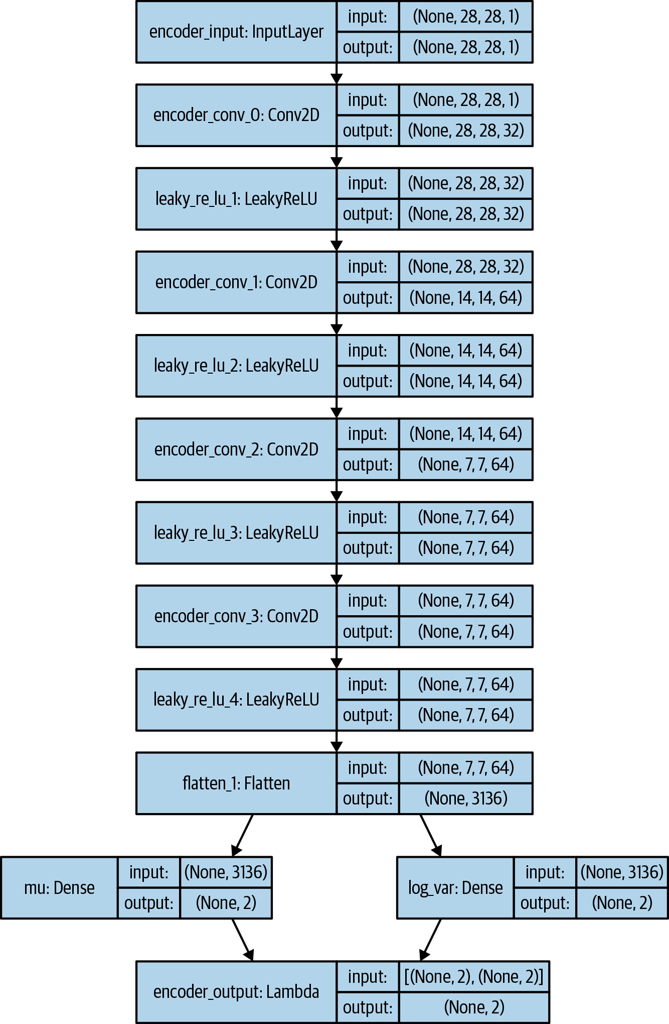
Figure 3-13. Diagram of the VAE encoder
The Loss Function
Previously, our loss function only consisted of the RMSE loss between images and their reconstruction after being passed through the encoder and decoder. This reconstruction loss also appears in a variational autoencoder, but we require one extra component: the Kullback–Leibler (KL) divergence.
KL divergence is a way of measuring how much one probability distribution differs from another. In a VAE, we want to measure how different our normal distribution with parameters mu and log_var is from the standard normal distribution. In this special case, the KL divergence has the closed form:
kl_loss = -0.5 * sum(1 + log_var - mu ^ 2 - exp(log_var))
or in mathematical notation:
The sum is taken over all the dimensions in the latent space. kl_loss is minimized to 0 when mu = 0 and log_var = 0 for all dimensions. As these two terms start to differ from 0, kl_loss increases.
In summary, the KL divergence term penalizes the network for encoding observations to mu and log_var variables that differ significantly from the parameters of a standard normal distribution, namely mu = 0 and log_var = 0.
Again, relating this back to our story, this term represents Epsilon’s annoyance at having to move the ladder away from the middle of the wall (mu different from 0) and also if Mr. N. Coder’s confidence in the marker position isn’t just right (log_var different from 0), both of which incur a cost.
Why does this addition to the loss function help?
First, we now have a well-defined distribution that we can use for choosing points in the latent space—the standard normal distribution. If we sample from this distribution, we know that we’re very likely to get a point that lies within the limits of what the VAE is used to seeing. Secondly, since this term tries to force all encoded distributions toward the standard normal distribution, there is less chance that large gaps will form between point clusters. Instead, the encoder will try to use the space around the origin symmetrically and efficiently.
In the code, the loss function for a VAE is simply the addition of the reconstruction loss and the KL divergence loss term. We weight the reconstruction loss with a term, r_loss_factor, that ensures that it is well balanced with the KL divergence loss. If we weight the reconstruction loss too heavily, the KL loss will not have the desired regulatory effect and we will see the same problems that we experienced with the plain autoencoder. If the weighting term is too small, the KL divergence loss will dominate and the reconstructed images will be poor. This weighting term is one of the parameters to tune when you’re training your VAE.
Example 3-8 shows how we include the KL divergence term in our loss function.
Example 3-8. Including KL divergence in the loss function
### COMPILATIONoptimizer=Adam(lr=learning_rate)defvae_r_loss(y_true,y_pred):r_loss=K.mean(K.square(y_true-y_pred),axis=[1,2,3])returnr_loss_factor*r_lossdefvae_kl_loss(y_true,y_pred):kl_loss=-0.5*K.sum(1+self.log_var-K.square(self.mu)-K.exp(self.log_var),axis=1)returnkl_lossdefvae_loss(y_true,y_pred):r_loss=vae_r_loss(y_true,y_pred)kl_loss=vae_kl_loss(y_true,y_pred)returnr_loss+kl_lossoptimizer=Adam(lr=learning_rate)self.model.compile(optimizer=optimizer,loss=vae_loss,metrics=[vae_r_loss,vae_kl_loss])
Analysis of the Variational Autoencoder
All of the following analysis is available in the book repository, in the notebook 03_04_vae_digits_analysis.ipynb.
Referring back to Figure 3-10, we can see several changes in how the latent space is organized. The black dots show the mu values of each encoded image. The KL divergence loss term ensures that the mu and sigma values never stray too far from a standard normal. We can therefore sample from the standard normal distribution to generate new points in the space to be decoded (the red dots).
Secondly, there are not so many generated digits that are badly formed, since the latent space is now locally continuous due to fact that the encoder is now stochastic, rather than deterministic.
Finally, by coloring points in the latent space by digit (Figure 3-14), we can see that there is no preferential treatment of any one type. The righthand plot shows the space transformed into p-values, and we can see that each color is approximately equally represented. Again, it’s important to remember that the labels were not used at all during training—the VAE has learned the various forms of digits by itself in order to help minimize reconstruction loss.

Figure 3-14. The latent space of the VAE colored by digit
So far, all of our work on autoencoders and variational autoencoders has been limited to a latent space with two dimensions. This has helped us to visualize the inner workings of a VAE on the page and understand why the small tweaks that we made to the architecture of the autoencoder helped transform it into a more powerful class of network that can be used for generative modeling.
Let’s now turn our attention to a more complex dataset and see the amazing things that variational autoencoders can achieve when we increase the dimensionality of the latent space.
Using VAEs to Generate Faces
We shall be using the CelebFaces Attributes (CelebA) dataset to train our next variational autoencoder. This is a collection of over 200,000 color images of celebrity faces, each annotated with various labels (e.g., wearing hat, smiling, etc.). A few examples are shown in Figure 3-15.

Figure 3-15. Some examples from the CelebA dataset5
Of course, we don’t need the labels to train the VAE, but these will be useful later when we start exploring how these features are captured in the multidimensional latent space. Once our VAE is trained, we can sample from the latent space to generate new examples of celebrity faces.
Training the VAE
The network architecture for the faces model is similar to the digits example, with a few slight differences:
-
Our data now has three input channels (RGB) instead of one (grayscale). This means we need to change the number of channels in the final convolutional transpose layer of the decoder to
3. -
We shall be using a latent space with two hundred dimensions instead of two. Since faces are much more complex than digits, we increase the dimensionality of the latent space so that the network can encode a satisfactory amount of detail from the images.
-
There are batch normalization layers after each convolution layer to speed up training. Even though each batch takes a longer time to run, the number of batches required to reach the same loss is greatly reduced. Dropout layers are also used.
-
We increase the reconstruction loss factor to ten thousand. This is a parameter that requires tuning; for this dataset and architecture this value was found to generate good results.
-
We use a generator to feed images to the VAE from a folder, rather than loading all the images into memory up front. Since the VAE trains in batches, there is no need to load all the images into memory first, so instead we use the built-in
fit_generatormethod that Keras provides to read in images only when they are required for training.
The full architectures of the encoder and decoder are shown in Figures 3-16 and 3-17

Figure 3-16. The VAE encoder for the CelebA dataset

Figure 3-17. The VAE decoder for the CelebA dataset
To train the VAE on the CelebA dataset, run the Jupyter notebook 03_05_vae_faces_train.ipynb from the book repository. After around five epochs of training your VAE should be able to produce novel images of celebrity faces!
Analysis of the VAE
You can replicate the analysis that follows by running the notebook 03_06_vae_faces_analysis.ipynb, once you have trained the VAE. Many of the ideas in this section were inspired by a 2016 paper by Xianxu Hou et al.6
First, let’s take a look at a sample of reconstructed faces. The top row in Figure 3-18 shows the original images and the bottom row shows the reconstructions once they have passed through the encoder and decoder.

Figure 3-18. Reconstructed faces, after passing through the encoder and decoder
We can see that the VAE has successfully captured the key features of each face—the angle of the head, the hairstyle, the expression, etc. Some of the fine detail is missing, but it is important to remember that the aim of building variational autoencoders isn’t to achieve perfect reconstruction loss. Our end goal is to sample from the latent space in order to generate new faces.
For this to be possible we must check that the distribution of points in the latent space approximately resembles a multivariate standard normal distribution. Since we cannot view all dimensions simultaneously, we can instead check the distribution of each latent dimension individually. If we see any dimensions that are significantly different from a standard normal distribution, we should probably reduce the reconstruction loss factor, since the KL divergence term isn’t having enough effect.
The first 50 dimensions in our latent space are shown in Figure 3-19. There aren’t any distributions that stand out as being significantly different from the standard normal, so we can move on to generating some faces!

Figure 3-19. Distributions of points for the first 50 dimensions in the latent space
Generating New Faces
To generate new faces, we can use the code in Example 3-9.
Example 3-9. Generating new faces from the latent space
n_to_show=30znew=np.random.normal(size=(n_to_show,VAE.z_dim))reconst=VAE.decoder.predict(np.array(znew))fig=plt.figure(figsize=(18,5))fig.subplots_adjust(hspace=0.4,wspace=0.4)foriinrange(n_to_show):ax=fig.add_subplot(3,10,i+1)ax.imshow(reconst[i,:,:,:])ax.axis('off')plt.show()
We sample 30 points from a standard normal distribution with 200 dimensions…
…then pass these points to the decoder.
The resulting output is a 128 × 128 × 3 image that we can view.
The output is shown in Figure 3-20.

Figure 3-20. New generated faces
Amazingly, the VAE is able to take the set of points that we sampled and convert each into a convincing image of a person’s face. While the images are not perfect, they are a giant leap forward from the Naive Bayes model that we started exploring in Chapter 1. The Naive Bayes model faced the problem of not being able to capture dependency between adjacent pixels, since it had no notion of higher-level features such as sunglasses or brown hair. The VAE doesn’t suffer from this problem, since the convolutional layers of the encoder are designed to translate low-level pixels into high-level features and the decoder is trained to perform the opposite task of translating the high-level features in the latent space back to raw pixels.
Latent Space Arithmetic
One benefit of mapping images into a lower-dimensional space is that we can perform arithmetic on vectors in this latent space that has a visual analogue when decoded back into the original image domain.
For example, suppose we want to take an image of somebody who looks sad and give them a smile. To do this we first need to find a vector in the latent space that points in the direction of increasing smile. Adding this vector to the encoding of the original image in the latent space will give us a new point which, when decoded, should give us a more smiley version of the original image.
So how can we find the smile vector? Each image in the CelebA dataset is labeled with attributes, one of which is smiling. If we take the average position of encoded images in the latent space with the attribute smiling and subtract the average position of encoded images that do not have the attribute smiling, we will obtain the vector that points from not smiling to smiling, which is exactly what we need.
Conceptually, we are performing the following vector arithmetic in the latent space, where alpha is a factor that determines how much of the feature vector is added or subtracted:
z_new = z + alpha * feature_vector
Let’s see this in action. Figure 3-21 shows several images that have been encoded into the latent space. We then add or subtract multiples of a certain vector (e.g., smile, blonde, male, eyeglasses) to obtain different versions of the image, with only the relevant feature changed.

Figure 3-21. Adding and subtracting features to and from faces
It is quite remarkable that even though we are moving the point a significantly large distance in the latent space, the core image barely changes, except for the one feature that we want to manipulate. This demonstrates the power of variational autoencoders for capturing and adjusting high-level features in images.
Morphing Between Faces
We can use a similar idea to morph between two faces. Imagine two points in the latent space, A and B, that represent two images. If you started at point A and walked toward point B in a straight line, decoding each point on the line as you went, you would see a gradual transition from the starting face to the end face.
Mathematically, we are traversing a straight line, which can be described by the following equation:
z_new = z_A * (1- alpha) + z_B * alpha
Here, alpha is a number between 0 and 1 that determines how far along the line we are, away from point A.
Figure 3-22 shows this process in action. We take two images, encode them into the latent space, and then decode points along the straight line between them at regular intervals.

Figure 3-22. Morphing between two faces
It is worth noting the smoothness of the transition—even where there are multiple features to change simultaneously (e.g., removal of glasses, hair color, gender), the VAE manages to achieve this fluidly, showing that the latent space of the VAE is truly a continuous space that can be traversed and explored to generate a multitude of different human faces.
Summary
In this chapter we have seen how variational autoencoders are a powerful tool in the generative modeling toolbox. We started by exploring how plain autoencoders can be used to map high-dimensional images into a low-dimensional latent space, so that high-level features can be extracted from the individually uninformative pixels. However, like with the Coder brothers’ art exhibition, we quickly found that there were some drawbacks to using plain autoencoders as a generative model—sampling from the learned latent space was problematic, for a number of reasons.
Variational autoencoders solve these problems, by introducing randomness into the model and constraining how points in the latent space are distributed. We saw that with a few minor adjustments, we can transform our autoencoder into a variational autoencoder, thus giving it the power to be a generative model.
Finally, we applied our new technique to the problem of face generation and saw how we can simply choose points from a standard normal distribution to generate new faces. Moreover, by performing vector arithmetic within the latent space, we can achieve some amazing effects, such as face morphing and feature manipulation. With these features, it is easy to see why VAEs have become a prominent technique for generative modeling in recent years.
In the next chapter, we shall explore a different kind of generative model that has attracted an even greater amount of attention: the generative adversarial network.
1 Diederik P. Kingma and Max Welling, “Auto-Encoding Variational Bayes,” 20 December 2013, https://arxiv.org/abs/1312.6114.
2 Source: Vincent Dumoulin and Francesco Visin, “A Guide to Convolution Arithmetic for Deep Learning,” 12 January 2018, https://arxiv.org/pdf/1603.07285.pdf.
3 Source: Wikipedia, http://bit.ly/2ZDWRJv.
5 Source: Liu et al., 2015, http://mmlab.ie.cuhk.edu.hk/projects/CelebA.html.
6 Xianxu Hou et al., “Deep Feature Consistent Variational Autoencoder,” 2 October 2016, https://arxiv.org/abs/1610.00291.