
Chapter 7. Compose
Alongside visual art and creative writing, musical composition is another core act of creativity that we consider to be uniquely human.
For a machine to compose music that is pleasing to our ear, it must master many of the same technical challenges that we saw in the previous chapter in relation to text. In particular, our model must be able to learn from and re-create the sequential structure of music and must also be able to choose from a discrete set of possibilities for subsequent notes.
However, musical generation presents additional challenges that are not required for text generation, namely pitch and rhythm. Music is often polyphonic—that is, there are several streams of notes played simultaneously on different instruments, which combine to create harmonies that are either dissonant (clashing) or consonant (harmonious). Text generation only requires us to handle a single stream of text, rather than the parallel streams of chords that are present in music.
Also, text generation can be handled one word at a time. We must consider carefully if this is an appropriate way to process musical data, as much of the interest that stems from listening to music is in the interplay between different rhythms across the ensemble. A guitarist might play a flurry of quicker notes while the pianist holds a longer sustained chord, for example. Therefore, generating music note by note is complex, because we often do not want all the instruments to change note simultaneously.
We will start this chapter by simplifying the problem to focus on music generation for a single (monophonic) line of music. We will see that many of the RNN techniques from the previous chapter on text generation can also be used for music generation as the two tasks share many common themes. This chapter will also introduce the attention mechanism that will allow us to build RNNs that are able to choose which previous notes to focus on in order to predict which notes will appear next. Lastly, we’ll tackle the task of polyphonic music generation and explore how we can deploy an architecture based around GANs to create music for multiple voices.
Preliminaries
Anyone tackling the task of music generation must first have a basic understanding of musical theory. In this section we’ll go through the essential notation required to read music and how we can represent this numerically, in order to transform music into the input data required to train a generative model.
We’ll work through the notebook 07_01_notation_compose.ipynb in the book repository. Another excellent resource for getting started with music generation using Python is Sigurður Skúli’s blog post and accompanying GitHub repository.
The raw dataset that we shall be using is a set of MIDI files for the Cello Suites by J.S. Bach. You can use any dataset you wish, but if you want to work with this dataset, you can find instructions for downloading the MIDI files in the notebook.
To view and listen to the music generated by the model, you’ll need some software that can produce musical notation. MuseScore is a great tool for this purpose and can be downloaded for free.
Musical Notation
We’ll be using the Python library music21 to load the MIDI files into Python for processing. Example 7-1 shows how to load a MIDI file and visualize it (Figure 7-1), both as a score and as structured data.
Example 7-1. Importing a MIDI file
frommusic21importconverterdataset_name='cello'filename='cs1-2all'file="./data/{}/{}.mid".format(dataset_name,filename)original_score=converter.parse(file).chordify()

Figure 7-1. Musical notation
We use the chordify method to squash all simultaneously played notes into chords within a single part, rather than them being split between many parts. Since this piece is performed by one instrument (a cello), we are justified in doing this, though sometimes we may wish to keep the parts separate to generate music that is polyphonic in nature. This presents additional challenges that we shall tackle later on in this chapter.
The code in Example 7-2 loops through the score and extracts the pitch and duration for each note (and rest) in the piece into two lists. Individual notes in chords are separated by a dot, so that the whole chord can be stored as a single string. The number after each note name indicates the octave that the note is in—since the note names (A to G) repeat, this is needed to uniquely identify the pitch of the note. For example, G2 is an octave below G3.
Example 7-2. Extracting the data
notes=[]durations=[]forelementinoriginal_score.flat:ifisinstance(element,chord.Chord):notes.append('.'.join(n.nameWithOctaveforninelement.pitches))durations.append(element.duration.quarterLength)ifisinstance(element,note.Note):ifelement.isRest:notes.append(str(element.name))durations.append(element.duration.quarterLength)else:notes.append(str(element.nameWithOctave))durations.append(element.duration.quarterLength)
The output from this process is shown in Table 7-1.
The resulting dataset now looks a lot more like the text data that we have dealt with previously. The words are the pitches, and we should try to build a model that predicts the next pitch, given a sequence of previous pitches. The same idea can also be applied to the list of durations. Keras gives us the flexibility to be able to build a model that can handle the pitch and duration prediction simultaneously.
| Duration | Pitch |
|---|---|
| 0.25 | B3 |
| 1.0 | G2.D3.B3 |
| 0.25 | B3 |
| 0.25 | A3 |
| 0.25 | G3 |
| 0.25 | F#3 |
| 0.25 | G3 |
| 0.25 | D3 |
| 0.25 | E3 |
| 0.25 | F#3 |
| 0.25 | G3 |
| 0.25 | A3 |
Your First Music-Generating RNN
To create the dataset that will train the model, we first need to give each pitch and duration an integer value (Figure 7-2), exactly as we have done previously for each word in a text corpus. It doesn’t matter what these values are as we shall be using an embedding layer to transform the integer lookup values into vectors.

Figure 7-2. The integer lookup dictionaries for pitch and duration
We then create the training set by splitting the data into small chunks of 32 notes, with a response variable of the next note in the sequence (one-hot encoded), for both pitch and duration. One example of this is shown in Figure 7-3.

Figure 7-3. The inputs and outputs for the musical generative model
The model we will be building is a stacked LSTM network with an attention mechanism. In the previous chapter, we saw how we are able to stack LSTM layers by passing the hidden states of the previous layer as input to the next LSTM layer. Stacking layers in this way gives the model freedom to learn more sophisticated features from the data. In this section we will introduce the attention mechanism1 that now forms an integral part of most sophisticated sequential generative models. It has ultimately given rise to the transformer, a type of model based entirely on attention that doesn’t even require recurrent or convolutional layers. We will introduce the transformer architecture in more detail in Chapter 9.
For now, let’s focus on incorporating attention into a stacked LSTM network to try to predict the next note, given a sequence of previous notes.
Attention
The attention mechanism was originally applied to text translation problems—in particular, translating English sentences into French.
In the previous chapter, we saw how encoder–decoder networks can solve this kind of problem, by first passing the input sequence through an encoder to generate a context vector, then passing this vector through the decoder network to output the translated text. One observed problem with this approach is that the context vector can become a bottleneck. Information from the start of the source sentence can become diluted by the time it reaches the context vector, especially for long sentences. Therefore these kinds of encoder–decoder networks sometimes struggle to retain all the required information for the decoder to accurately translate the source.
As an example, suppose we want the model to translate the following sentence into German: I scored a penalty in the football match against England.
Clearly, the meaning of the entire sentence would be changed by replacing the word scored with missed. However, the final hidden state of the encoder may not be able to sufficiently retain this information, as the word scored appears early in the sentence.
The correct translation of the sentence is: Ich habe im Fußballspiel gegen England einen Elfmeter erzielt.
If we look at the correct German translation, we can see that the word for scored (erzielt) actually appears right at the end of the sentence! So not only would the model have to retain the fact that the penalty was scored rather than missed through the encoder, but also all the way through the decoder as well.
Exactly the same principle is true in music. To understand what note or sequence of notes is likely to follow from a particular given passage of music, it may be crucial to use information from far back in the sequence, not just the most recent information. For example, take the opening passage of the Prelude to Bach’s Cello Suite No. 1 (Figure 7-4).

Figure 7-4. The opening of Bach’s Cello Suite No. 1 (Prelude)
What note do you think comes next? Even if you have no musical training you may still be able to guess. If you said G (the same as the very first note of the piece), then you’d be correct. How did you know this? You may have been able to see that every bar and half bar starts with the same note and used this information to inform your decision. We want our model to be able to perform the same trick—in particular, we want it to not only care about the hidden state of the network now, but also to pay particular attention to the hidden state of the network eight notes ago, when the previous low G was registered.
The attention mechanism was proposed to solve this problem. Rather than only using the final hidden state of the encoder RNN as the context vector, the attention mechanism allows the model to create the context vector as a weighted sum of the hidden states of the encoder RNN at each previous timestep. The attention mechanism is just a set of layers that converts the previous encoder hidden states and current decoder hidden state into the summation weights that generate the context vector.
If this sounds confusing, don’t worry! We’ll start by seeing how to apply an attention mechanism after a simple recurrent layer (i.e., to solve the problem of predicting the next note of Bach’s Cello Suite No. 1), before we see how this extends to encoder–decoder networks, where we want to predict a whole sequence of subsequent notes, rather than just one.
Building an Attention Mechanism in Keras
First, let’s remind ourselves of how a standard recurrent layer can be used to predict the next note given a sequence of previous notes. Figure 7-5 shows how the input sequence (x1,…,xn) is fed to the layer one step at a time, continually updating the hidden state of the layer. The input sequence could be the note embeddings, or the hidden state sequence from a previous recurrent layer. The output from the recurrent layer is the final hidden state, a vector with the same length as the number of units. This can then be fed to a Dense layer with softmax output to predict a distribution for the next note in the sequence.

Figure 7-5. A recurrent layer for predicting the next note in a sequence, without attention
Figure 7-6 shows the same network, but this time with an attention mechanism applied to the hidden states of the recurrent layer.

Figure 7-6. A recurrent layer for predicting the next note in a sequence, with attention
Let’s walk through this process step by step:
-
First, each hidden state hj (a vector of length equal to the number of units in the recurrent layer) is passed through an alignment function a to generate a scalar, ej. In this example, this function is simply a densely connected layer with one output unit and a tanh activation function.
-
Next, the softmax function is applied to the vector e1,…,en to produce the vector of weights α1,…,αn.
-
Lastly, each hidden state vector hj is multiplied by its respective weight αj, and the results are then summed to give the context vector c (thus c has the same length as a hidden state vector).
The context vector can then be passed to a Dense layer with softmax output as usual, to output a distribution for the potential next note.
This network can be built in Keras as shown in Example 7-3.
Example 7-3. Building the RNN with attention
notes_in=Input(shape=(None,))durations_in=Input(shape=(None,))x1=Embedding(n_notes,embed_size)(notes_in)x2=Embedding(n_durations,embed_size)(durations_in)x=Concatenate()([x1,x2])x=LSTM(rnn_units,return_sequences=True)(x)x=LSTM(rnn_units,return_sequences=True)(x)e=Dense(1,activation='tanh')(x)e=Reshape([-1])(e)alpha=Activation('softmax')(e)c=Permute([2,1])(RepeatVector(rnn_units)(alpha))c=Multiply()([x,c])c=Lambda(lambdaxin:K.sum(xin,axis=1),output_shape=(rnn_units,))(c)notes_out=Dense(n_notes,activation='softmax',name='pitch')(c)durations_out=Dense(n_durations,activation='softmax',name='duration')(c)model=Model([notes_in,durations_in],[notes_out,durations_out])att_model=Model([notes_in,durations_in],alpha)opti=RMSprop(lr=0.001)model.compile(loss=['categorical_crossentropy','categorical_crossentropy'],optimizer=opti)

There are two inputs to the network: the sequence of previous note names and duration values. Notice how the sequence length isn’t specified—the attention mechanism does not require a fixed-length input, so we can leave this as variable.

The
Embeddinglayers convert the integer values of the note names and durations into vectors.
The vectors are concatenated to form one long vector that will be used as input into the recurrent layers.

Two stacked LSTM layers are used as the recurrent part of the network. Notice how we set
return_sequencestoTrueto make each layer pass the full sequence of hidden states to the next layer, rather than just the final hidden state.
The alignment function is just a
Denselayer with one output unit and tanh activation. We can use aReshapelayer to squash the output to a single vector, of length equal to the length of the input sequence (seq_length).
The weights are calculated through applying a softmax activation to the alignment values.

To get the weighted sum of the hidden states, we need to use a
RepeatVectorlayer to copy the weightsrnn_unitstimes to form a matrix of shape[rnn_units, seq_length], then transpose this matrix using aPermutelayer to get a matrix of shape[seq_length, rnn_units]. We can then multiply this matrix pointwise with the hidden states from the final LSTM layer, which also has shape[seq_length, rnn_units]. Finally, we use aLambdalayer to perform the summation along theseq_lengthaxis, to give the context vector of lengthrnn_units.
The network has a double-headed output, one for the next note name and one for the next note length.

The final model accepts the previous note names and note durations as input and outputs a distribution for the next note name and next note duration.

We also create a model that outputs the
alphalayer vector, so that we will be able to understand how the network is attributing weights to previous hidden states.
The model is compiled using
categorical_crossentropyfor both the note name and note duration output heads, as this is a multiclass classification problem.
A diagram of the full model built in Keras is shown in Figure 7-7.
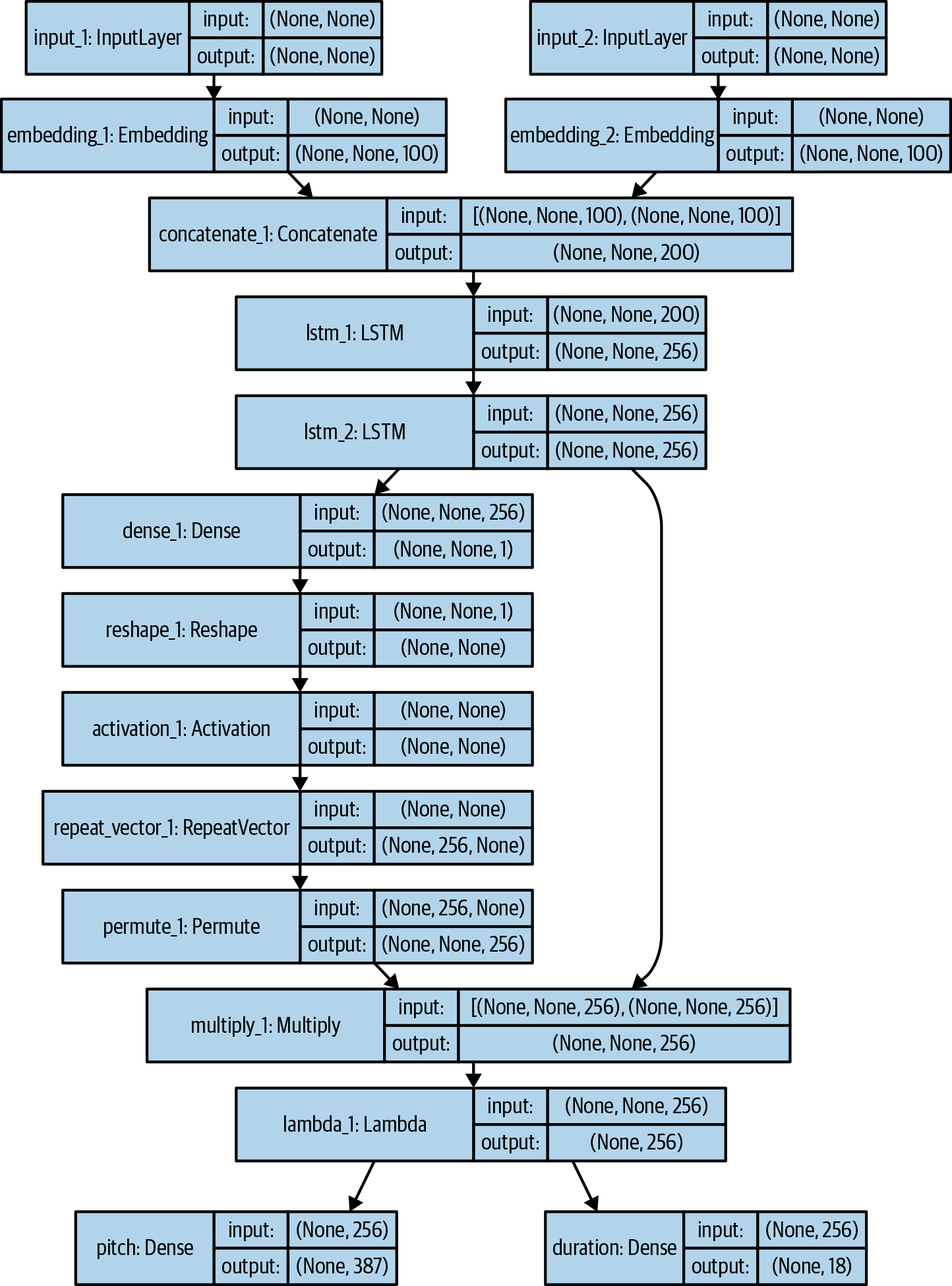
Figure 7-7. The LSTM model with attention for predicting the next note in a sequence
You can train this LSTM with attention by running the notebook called 07_02_lstm_compose_train.ipynb in the book repository.
Analysis of the RNN with Attention
The following analysis can be produced by running the notebook 07_03_lstm_compose_analysis.ipynb from the book repository, once you have trained your network.
We’ll start by generating some music from scratch, by seeding the network with only a sequence of <START> tokens (i.e., we are telling the model to assume it is starting from the beginning of the piece). Then we can generate a musical passage using the same iterative technique we used in Chapter 6 for generating text sequences, as follows:
-
Given the current sequence (of note names and note durations), the model predicts two distributions, for the next note name and duration.
-
We sample from both of these distributions, using a
temperatureparameter to control how much variation we would like in the sampling process. -
The chosen note is stored and its name and duration are appended to the respective sequences.
-
If the length of the sequence is now greater than the sequence length that the model was trained on, we remove one element from the start of the sequence.
-
The process repeats with the new sequence, and so on, for as many notes as we wish to generate.
Figure 7-8 shows examples of music generated from scratch by the model at various epochs of the training process.
Most of our analysis in this section will focus on the note pitch predictions, rather than rhythms, as for Bach’s Cello Suites the harmonic intricacies are more difficult to capture and therefore more worthy of investigation. However, you can also apply the same analysis to the rhythmic predictions of the model, which may be particularly relevant for other styles of music that you could use to train this model (such as a drum track).
There are several points to note about the generated passages in Figure 7-8. First, see how the music is becoming more sophisticated as training progresses. To begin with, the model plays it safe by sticking to the same group of notes and rhythms. By epoch 10, the model has begun to generate small runs of notes, and by epoch 20 it is producing interesting rhythms and is firmly established in a set key (E-flat major).

Figure 7-8. Some examples of passages generated by the model when seeded only with a sequence of <START> tokens; here we use a temperature of 0.5 for the note names and durations
Second, we can analyze the distribution of note pitches over time by plotting the predicted distribution at each timestep as a heatmap. Figure 7-9 shows this heatmap for the example from epoch 20 in Figure 7-8.

Figure 7-9. The distribution of possible next notes over time (at epoch 20): the darker the square, the more certain the model is that the next note is at this pitch
An interesting point to note here is that the model has clearly learned which notes belong to particular keys, as there are gaps in the distribution at notes that do not belong to the key. For example, there is a gray gap along the row for note 54 (corresponding to Gb/F#). This note is highly unlikely to appear in a piece of music in the key of E-flat major. Early on in the generation process (the lefthand side of the diagram) the key is not yet firmly established and therefore there is more uncertainty in how to choose the next note. As the piece progresses, the model settles on a key and certain notes become almost certain not to appear. What is remarkable is that the model hasn’t explicitly decided to set the music in a certain key at the beginning, but instead is literally making it up as it goes along, trying to choose the note that best fits with those it has chosen previously.
It is also worth pointing out that the model has learned Bach’s characteristic style of dropping to a low note on the cello to end a phrase and bouncing back up again to start the next. See how around note 20, the phrase ends on a low E-flat—it is common in the Bach Cello Suites to then return to a higher, more sonorous range of the instrument for the start of next phrase, which is exactly what the model predicts. There is a large gray gap between the low E-flat (pitch number 39) and the next note, which is predicted to be around pitch number 50, rather than continuing to rumble around the depths of the instrument.
Lastly, we should check to see if our attention mechanism is working as expected. Figure 7-10 shows the values of the alpha vector elements calculated by the network at each point in the generated sequence. The horizontal axis shows the generated sequence of notes; the vertical axis shows where the attention of the network was aimed when predicting each note along the horizontal axis (i.e., the alpha vector). The darker the square, the greater the attention placed on the hidden state corresponding to this point in the sequence.

Figure 7-10. Each square in the matrix indicates the amount of attention given to the hidden state of the network corresponding to the note on the vertical axis, at the point of predicting the note on the horizontal axis; the more red the square, the more attention was given
We can see that for the second note of the piece (B-3 = B-flat), the network chose to place almost all of its attention on the fact that the first note of the piece was also B-3. This makes sense; if you know that the first note is a B-flat, you will probably use this information to inform your decision about the next note.
As we move through the next few notes, the network spreads its attention roughly equally among previous notes—however, it rarely places any weight on notes more than six notes ago. Again, this makes sense; there is probably enough information contained in the previous six hidden states to understand how the phrase should continue.
There are also examples of where the network has chosen to ignore a certain note nearby, as it doesn’t add any additional information to its understanding of the phrase. For example, take a look inside the white box marked in the center of the diagram, and note how there is a strip of boxes in the middle that cuts through the usual pattern of looking back at the previous four to six notes. Why would the network willingly choose to ignore this note when deciding how to continue the phrase?
If you look across to see which note this corresponds to, you can see that it is the first of three E-3 (E-flat) notes. The model has chosen to ignore this because the note prior to this is also an E-flat, an octave lower (E-2). The hidden state of the network at this point will provide ample information for the model to understand that E-flat is an important note in this passage, and therefore the model does not need to pay attention to the subsequent higher E-flat, as it doesn’t add any extra information.
Additional evidence that the model has started to understand the concept of an octave can be seen inside the green box below and to the right. Here the model has chosen to ignore the low G (G2) because the note prior to this was also a G (G3), an octave higher. Remember we haven’t told the model anything about which notes are related through octaves—it has worked this out for itself just by studying the music of J.S. Bach, which is remarkable.
Attention in Encoder–Decoder Networks
The attention mechanism is a powerful tool that helps the network decide which previous states of the recurrent layer are important for predicting the continuation of a sequence. So far, we have seen this for one-note-ahead predictions. However, we may also wish to build attention into encoder–decoder networks, where we predict a sequence of future notes by using an RNN decoder, rather than building up sequences one note at a time.
To recap, Figure 7-11 shows how a standard encoder–decoder model for music generation might look, without attention—the kind that we introduced in Chapter 6.
Figure 7-12 shows the same network, but with an attention mechanism between the encoder and the decoder.

Figure 7-11. The standard encoder–decoder model

Figure 7-12. An encoder–decoder model with attention
The attention mechanism works in exactly the same way as we have seen previously, with one alteration: the hidden state of the decoder is also rolled into the mechanism so that the model is able to decide where to focus its attention not only through the previous encoder hidden states, but also from the current decoder hidden state. Figure 7-13 shows the inner workings of an attention module within an encoder–decoder framework.

Figure 7-13. An attention mechanism within the context of an encoder-decoder network, connected to decoder cell i
While there are many copies of the attention mechanism within the encoder–decoder network, they all share the same weights, so there is no extra overhead in the number of parameters to be learned. The only change is that now, the decoder hidden state is rolled into the attention calculations (the red lines in the diagram). This slightly changes the equations to incorporate an extra index (i) to specify the step of the decoder.
Also notice how in Figure 7-11 we use the final state of the encoder to initialize the hidden state of the decoder. In an encoder–decoder with attention, we instead initialize the decoder using the built-in standard initializers for a recurrent layer. The context vector ci is concatenated with the incoming data yi–1 to form an extended vector of data into each cell of the decoder. Thus, we treat the context vectors as additional data to be fed into the decoder.
Generating Polyphonic Music
The RNN with attention mechanism framework that we have explored in this section works well for single-line (monophonic) music, but could it be adapted to multiline (polyphonic) music?
The RNN framework is certainly flexible enough to conceive of an architecture whereby multiple lines of music are generated simultaneously, through a recurrent mechanism. But as it stands, our current dataset isn’t well set up for this, as we are storing chords as single entities rather than parts that consist of multiple individual notes. There is no way for our current RNN to know, for example, that a C-major chord (C, E, and G) is actually very close to an A-minor chord (A, C, and E)—only one note would need to change, the G to an A. Instead, it treats both as two distinct elements to be predicted independently.
Ideally, we would like to design a network that can accept multiple channels of music as individual streams and learn how these streams should interact with each other to generate beautiful-sounding music, rather than disharmonious noise.
Doesn’t this sound a bit like generating images? For image generation we have three channels (red, green, and blue), and we want the network to learn how to combine these channels to generate beautiful-looking images, rather than random pixelated noise.
In fact, as we shall see in the next section, we can treat music generation directly as an image generation problem. This means that instead of using recurrent networks we can apply the same convolutional-based techniques that worked so well for image generation problems to music—in particular, GANs.
Before we explore this new architecture, there is just enough time to visit the concert hall, where a performance is about to begin…
The Musical Organ
The conductor taps his baton twice on the podium. The performance is about to begin. In front of him sits an orchestra. However, this orchestra isn’t about to launch into a Beethoven symphony or a Tchaikovsky overture. This orchestra composes original music live during the performance and is powered entirely by a set of players giving instructions to a huge Musical Organ (MuseGAN for short) in the middle of the stage, which converts these instructions into beautiful music for the pleasure of the audience. The orchestra can be trained to generate music in a particular style, and no two performances are ever the same.
The 128 players in the orchestra are divided into 4 equal sections of 32 players. Each section gives instructions to the MuseGAN and has a distinct responsibility within the orchestra.
The style section is in charge of producing the overall musical stylistic flair of the performance. In many ways, it has the easiest job of all the sections as each player simply has to generate a single instruction at the start of the concert that is then continually fed to the MuseGAN throughout the performance.
The groove section has a similar job, but each player produces several instructions: one for each of the distinct musical tracks that are output by the MuseGAN. For example, in one concert, each member of the groove section produced five instructions, one for each of the vocal, piano, string, bass, and drum tracks. Thus, their job is to provide the groove for each individual instrumental sound that is then constant throughout the performance.
The style and groove sections do not change their instructions throughout the piece. The dynamic element of the performance is provided by the final two sections, which ensure that the music is constantly changing with each bar that goes by. A bar (or measure) is a small unit of music that contains a fixed, small number of beats. For example, if you can count 1, 2, 1, 2 along to a piece of music, then there are two beats in each bar and you’re probably listening to a march. If you can count 1, 2, 3, 1, 2, 3, then there are three beats to each bar and you may be listening to a waltz.
The players in the chords section change their instructions at the start of each bar. This has the effect of giving each bar a distinct musical character, for example, through a change of chord. The players in the chords section only produce one instruction per bar that then applies to every instrumental track.
The players in the melody section have the most exhausting job, because they give different instructions to each instrumental track at the start of every bar throughout the piece. These players have the most fine-grained control over the music, and this can therefore be thought of as the section that provides the melodic interest.
This completes the description of the orchestra. We can summarize the responsibilities of each section as shown in Table 7-2.
| Instructions change with each bar? | Different instruction per track? | |
|---|---|---|
| Style | X | X |
| Groove | X | ✓ |
| Chords | ✓ | X |
| Melody | ✓ | ✓ |
It is up to the MuseGAN to generate the next bar of music, given the current set of 128 instructions (one from each player). Training the MuseGAN to do this isn’t easy. Initially the instrument only produces horrendous noise, as it has no way to understand how it should interpret the instructions to produce bars that are indistinguishable from genuine music.
This is where the conductor comes in. The conductor tells the MuseGAN when the music it is producing is clearly distinguishable from real music, and the MuseGAN then adapts its internal wiring to be more likely to fool the conductor the next time around. The conductor and the MuseGAN use exactly the same process as we saw in Chapter 4, when Di and Gene worked together to continuously improve the photos of ganimals taken by Gene.
The MuseGAN players tour the world giving concerts in any style where there is sufficient existing music to train the MuseGAN. In the next section we’ll see how we can build a MuseGAN using Keras, to learn how to generate realistic polyphonic music.
Your First MuseGAN
The MuseGAN was introduced in the 2017 paper “MuseGAN: Multi-Track Sequential Generative Adversarial Networks for Symbolic Music Generation and Accompaniment.”2 The authors show how it is possible to train a model to generate polyphonic, multitrack, multibar music through a novel GAN framework. Moreover, they show how, by dividing up the responsibilities of the noise vectors that feed the generator, they are able to maintain fine-grained control over the high-level temporal and track-based features of the music.
To begin this project, you’ll first need to download the MIDI files that we’ll be using to train the MuseGAN. We’ll use a dataset of 229 J.S. Bach chorales for four voices, available on GitHub. Download this dataset and place it inside the data folder of the book repository, in a folder called chorales. The dataset consists of an array of four numbers for each timestep: the MIDI note pitches of each of the four voices. A timestep in this dataset is equal to a 16th note (a semiquaver). So, for example, in a single bar of 4 quarter (crotchet) beats, there would be 16 timesteps. Also, the dataset is automatically split into train, validation, and test sets. We will be using the train dataset to train the MuseGAN.
We first need to get the data into the correct shape to feed the GAN. In this example, we’ll generate two bars of music, so we’ll first extract only the first two bars of each chorale. Figure 7-14 shows how two bars of raw data are converted into the transformed dataset that will feed the GAN with the corresponding musical notation.
Each bar consists of 16 timesteps and there are a potential 84 pitches across the 4 tracks. Therefore, a suitable shape for the transformed data is:
[batch_size, n_bars, n_steps_per_bar, n_pitches, n_tracks]
where
n_bars = 2
n_steps_per_bar = 16
n_pitches = 84
n_tracks = 4
To get the data into this shape, we one-hot encode the pitch numbers into a vector of length 84 and split each sequence of notes into two groups of 16, to replicate 2 bars.3
Now that we have transformed our dataset, let’s take a look at the overall structure of the MuseGAN, starting with the generator.

Figure 7-14. Example of MuseGAN raw data
The MuseGAN Generator
Like all GANs, the MuseGAN consists of a generator and a critic. The generator tries to fool the critic with its musical creations, and the critic tries to prevent this from happening by ensuring it is able to tell the difference between the generator’s forged Bach chorales and the real thing.
Where the MuseGAN is different is the fact that the generator doesn’t just accept a single noise vector as input, but instead has four separate inputs, which correspond to the four sections of the orchestra in the story—chords, style, melody, and groove. By manipulating each of these inputs independently we can change high-level properties of the generated music.
A high-level view of the generator is shown in Figure 7-15.

Figure 7-15. High-level diagram of the MuseGAN generator
The diagram shows how the chords and melody inputs are first passed through a temporal network that outputs a tensor with one of the dimensions equal to the number of bars to be generated. The style and groove inputs are not stretched temporally in this way, as they remain constant through the piece.
Then, to generate a particular bar for a particular track, the relevant vectors from the chords, style, melody, and groove parts of the network are concatenated to form a longer vector. This is then passed to a bar generator, which ultimately outputs the specified bar for the specified track.
By concatenating the generated bars for all tracks, we create a score that can be compared with real scores by the critic. You can start training the MuseGAN using the notebook 07_04_musegan_train.ipynb in the book repository. The parameters to the model are given in Example 7-4.
Example 7-4. Defining the MuseGAN
BATCH_SIZE=64n_bars=2n_steps_per_bar=16n_pitches=84n_tracks=4z_dim=32gan=MuseGAN(input_dim=data_binary.shape[1:],critic_learning_rate=0.001,generator_learning_rate=0.001,optimiser='adam',grad_weight=10,z_dim=32,batch_size=64,n_tracks=4,n_bars=2,n_steps_per_bar=16,n_pitches=84)
Chords, Style, Melody, and Groove
Let’s now take a closer look at the four different inputs that feed the generator.
Chords
The chords input is a vector of length 32 (z_dim). We need to output a different vector for every bar, as its job is to control the general dynamic nature of the music over time. Note that while this is labeled chords_input, it really could control anything about the music that changes per bar, such as general rhythmic style, without being specific to any particular track.
The way this is achieved is with a neural network consisting of convolutional transpose layers that we call the temporal network. The Keras code to build this is shown in Example 7-5.
Example 7-5. Building the temporal network
defconv_t(self,x,f,k,s,a,p,bn):x=Conv2DTranspose(filters=f,kernel_size=k,padding=p,strides=s,kernel_initializer=self.weight_init)(x)ifbn:x=BatchNormalization(momentum=0.9)(x)ifa=='relu':x=Activation(a)(x)elifa=='lrelu':x=LeakyReLU()(x)returnxdefTemporalNetwork(self):input_layer=Input(shape=(self.z_dim,),name='temporal_input')x=Reshape([1,1,self.z_dim])(input_layer)x=self.conv_t(x,f=1024,k=(2,1),s=(1,1),a='relu',p='valid',bn=True)x=self.conv_t(x,f=self.z_dim,k=(self.n_bars-1,1),s=(1,1),a='relu',p='valid',bn=True)output_layer=Reshape([self.n_bars,self.z_dim])(x)returnModel(input_layer,output_layer)
The input to the temporal network is a vector of length 32 (
z_dim).We reshape this vector to a 1 × 1 tensor with 32 channels, so that we can apply convolutional transpose operations to it.
We apply
Conv2DTransposelayers to expand the size of the tensor along one axis, so that it is the same length asn_bars.We remove the unnecessary extra dimension with a
Reshapelayer.
The reason we use convolutional operations rather than requiring two independent chord vectors into the network is because we would like the network to learn how one bar should follow on from another in a consistent way. Using a neural network to expand the input vector along the time axis means the model has a chance to learn how music flows across bars, rather than treating each bar as completely independent of the last.
Style
The style input is also a vector of length z_dim. This is carried across to the bar generator without any change, as it is independent of the track and bar. In other words, the bar generator should use this vector to establish consistency between bars and tracks.
Melody
The melody input is an array of shape [n_tracks, z_dim]—that is, we provide the model with a random noise vector of length z_dim for each track.
Each of these vectors is passed through its own copy of the temporal network specified previously. Note that the weights of these copies are not shared. The output is therefore a vector of length z_dim for every track of every bar. This way, the bar generator will be able to use this vector to fine-tune the content of every single bar and track independently.
Groove
The groove input is also an array of shape [n_tracks, z_dim]—a random noise vector of length z_dim for each track. Unlike the melody input, these are not passed through the temporal network but instead are fed straight through to the bar generator unchanged, just like the style vector. However, unlike in the style vector there is a distinct groove input for every track, meaning that we can use these vectors to adjust the overall output for each track independently.
The Bar Generator
The bar generator converts a vector of length 4 * z_dim to a single bar for a single track—i.e., a tensor of shape [1, n_steps_per_bar, n_pitches, 1]. The input vector is created through the concatenation of the four relevant chord, style, melody, and groove vectors, each of length z_dim.
The bar generator is a neural network that uses convolutional transpose layers to expand the time and pitch dimensions. We will be creating one bar generator for every track, and weights are not shared. The Keras code to build a bar generator is given in Example 7-6.
Example 7-6. Building the bar generator
defBarGenerator(self):input_layer=Input(shape=(self.z_dim*4,),name='bar_generator_input')x=Dense(1024)(input_layer)x=BatchNormalization(momentum=0.9)(x)x=Activation('relu')(x)x=Reshape([2,1,512])(x)x=self.conv_t(x,f=512,k=(2,1),s=(2,1),a='relu',p='same',bn=True)x=self.conv_t(x,f=256,k=(2,1),s=(2,1),a='relu',p='same',bn=True)x=self.conv_t(x,f=256,k=(2,1),s=(2,1),a='relu',p='same',bn=True)x=self.conv_t(x,f=256,k=(1,7),s=(1,7),a='relu',p='same',bn=True)x=self.conv_t(x,f=1,k=(1,12),s=(1,12),a='tanh',p='same',bn=False)output_layer=Reshape([1,self.n_steps_per_bar,self.n_pitches,1])(x)returnModel(input_layer,output_layer)
The input to the bar generator is a vector of length
4 * z_dim.After passing through a
Denselayer, we reshape the tensor to prepare it for the convolutional transpose operations.First we expand the tensor along the timestep axis…
…then along the pitch axis.
The final layer has a tanh activation applied, as we will be using a WGAN-GP (which requires tanh output activation) to train the network.
The tensor is reshaped to add two extra dimensions of size 1, to prepare it for concatenation with other bars and tracks.
Putting It All Together
Ultimately the MuseGAN has one single generator that incorporates all of the temporal networks and bar generators. This network takes the four input tensors and converts them into a multitrack, multibar score. The Keras code to build the overall generator is provided in Example 7-7.
Example 7-7. Building the MuseGAN generator
chords_input=Input(shape=(self.z_dim,),name='chords_input')style_input=Input(shape=(self.z_dim,),name='style_input')melody_input=Input(shape=(self.n_tracks,self.z_dim),name='melody_input')groove_input=Input(shape=(self.n_tracks,self.z_dim),name='groove_input')# CHORDS -> TEMPORAL NETWORKself.chords_tempNetwork=self.TemporalNetwork()self.chords_tempNetwork.name='temporal_network'chords_over_time=self.chords_tempNetwork(chords_input)# [n_bars, z_dim]# MELODY -> TEMPORAL NETWORKmelody_over_time=[None]*self.n_tracks# list of n_tracks [n_bars, z_dim] tensorsself.melody_tempNetwork=[None]*self.n_tracksfortrackinrange(self.n_tracks):self.melody_tempNetwork[track]=self.TemporalNetwork()melody_track=Lambda(lambdax:x[:,track,:])(melody_input)melody_over_time[track]=self.melody_tempNetwork[track](melody_track)# CREATE BAR GENERATOR FOR EACH TRACKself.barGen=[None]*self.n_tracksfortrackinrange(self.n_tracks):self.barGen[track]=self.BarGenerator()# CREATE OUTPUT FOR EVERY TRACK AND BARbars_output=[None]*self.n_barsforbarinrange(self.n_bars):track_output=[None]*self.n_tracksc=Lambda(lambdax:x[:,bar,:],name='chords_input_bar_'+str(bar))(chords_over_time)s=style_inputfortrackinrange(self.n_tracks):m=Lambda(lambdax:x[:,bar,:])(melody_over_time[track])g=Lambda(lambdax:x[:,track,:])(groove_input)z_input=Concatenate(axis=1,name='total_input_bar_{}_track_{}'.format(bar,track))([c,s,m,g])track_output[track]=self.barGen[track](z_input)bars_output[bar]=Concatenate(axis=-1)(track_output)generator_output=Concatenate(axis=1,name='concat_bars')(bars_output)self.generator=Model([chords_input,style_input,melody_input,groove_input],generator_output)
The inputs to the generator are defined.
Pass the chords input through the temporal network.
Pass the melody input through the temporal network.
Create an independent bar generator network for every track.
Loop over the tracks and bars, creating a generated bar for each combination.
Concatenate everything together to form a single output tensor.
The MuseGAN model takes four distinct noise tensors as input and outputs a generated multitrack, multibar score.
The Critic
In comparison to the generator, the critic architecture is much more straightforward (as is often the case with GANs).
The critic tries to distinguish full multitrack, multibar scores created by the generator from real excepts from the Bach chorales. It is a convolutional neural network, consisting mostly of Conv3D layers that collapse the score into a single output prediction. So far, we have only worked with Conv2D layers, applicable to three-dimensional input images (width, height, channels). Here we have to use Conv3D layers, which are analogous to Conv2D layers but accept four-dimensional input tensors (n_bars, n_steps_per_bar, n_pitches, n_tracks).
Also, we do not use batch normalization layers in the critic as we will be using the WGAN-GP framework for training the GAN, which forbids this.
The Keras code to build the critic is given in Example 7-8.
Example 7-8. Building the MuseGAN critic
defconv(self,x,f,k,s,a,p):x=Conv3D(filters=f,kernel_size=k,padding=p,strides=s,kernel_initializer=self.weight_init)(x)ifa=='relu':x=Activation(a)(x)elifa=='lrelu':x=LeakyReLU()(x)returnxcritic_input=Input(shape=self.input_dim,name='critic_input')x=critic_inputx=self.conv(x,f=128,k=(2,1,1),s=(1,1,1),a='lrelu',p='valid')x=self.conv(x,f=128,k=(self.n_bars-1,1,1),s=(1,1,1),a='lrelu',p='valid')x=self.conv(x,f=128,k=(1,1,12),s=(1,1,12),a='lrelu',p='same')x=self.conv(x,f=128,k=(1,1,7),s=(1,1,7),a='lrelu',p='same')x=self.conv(x,f=128,k=(1,2,1),s=(1,2,1),a='lrelu',p='same')x=self.conv(x,f=128,k=(1,2,1),s=(1,2,1),a='lrelu',p='same')x=self.conv(x,f=256,k=(1,4,1),s=(1,2,1),a='lrelu',p='same')x=self.conv(x,f=512,k=(1,3,1),s=(1,2,1),a='lrelu',p='same')x=Flatten()(x)x=Dense(1024,kernel_initializer=self.weight_init)(x)x=LeakyReLU()(x)critic_output=Dense(1,activation=None,kernel_initializer=self.weight_init)(x)self.critic=Model(critic_input,critic_output)
The input to the critic is an array of multitrack, multibar scores, each of shape
[n_bars, n_steps_per_bar, n_pitches, n_tracks].First, we collapse the tensor along the bar axis. We apply
Conv3Dlayers throughout the critic as we are working with 4D tensors.Next, we collapse the tensor along the pitch axis.
Finally, we collapse the tensor along the timesteps axis.
The output is a
Denselayer with a single unit and no activation function, as required by the WGAN-GP framework.
Analysis of the MuseGAN
We can perform some experiments with our MuseGAN by generating a score, then tweaking some of the input noise parameters to see the effect on the output.
The output from the generator is an array of values in the range [–1, 1] (due to the tanh activation function of the final layer). To convert this to a single note for each track, we choose the note with the maximum value over all 84 pitches for each timestep. In the original MuseGAN paper the authors use a threshold of 0, as each track can contain multiple notes; however, in this setting we can simply take the maximum, to guarantee exactly one note per timestep per track, as is the case for the Bach chorales.
Figure 7-16 shows a score that has been generated by the model from random normally distributed noise vectors (top left). We can find the closest score in the dataset (by Euclidean distance) and check that our generated score isn’t a copy of a piece of music that already exists in the dataset—the closest score is shown just below it, and we can see that it does not resemble our generated score.

Figure 7-16. Example of a MuseGAN predicted score, showing the closest real score in the training data and how the generated score is affected by changing the input noise
Let’s now play around with the input noise to tweak our generated score. First, we can try changing the noise vector—the bottom-left score in Figure 7-16 shows the result. We can see that every track has changed, as expected, and also that the two bars exhibit different properties. In the second bar, the baseline is more dynamic and the top line is higher in pitch than in the first bar.
When we change the style vector (top right), both bars change in a similar way. There is no great difference in style between the two bars, but the whole passage has changed from the original generated score.
We can also alter tracks individually, through the melody and groove inputs. In Figure 7-16 we can see the effect of changing just the melody noise input for the top line of music. All other parts remain unaffected, but the top-line notes change significantly. Also, we can see a rhythmic change between the two bars in the top line: the second bar is more dynamic, containing faster notes than the first bar.
Lastly, the bottom-right score in the diagram shows the predicted score when we alter the groove input parameter for only the baseline. Again, all other parts remain unaffected, but the baseline is different. Moreover, the overall pattern of the baseline remains similar between bars, as we would expect.
This shows how each of the input parameters can be used to directly influence high-level features of the generated musical sequence, in much the same way as we were able to adjust the latent vectors of VAEs and GANs in previous chapters to alter the appearance of a generated image. One drawback to the model is that the number of bars to generate must be specified up front. The tackle this, the authors show a extension to the model that allows previous bars to be fed in as input, therefore allowing the model to generate long-form scores by continually feeding the most recent predicted bars back into the model as additional input.
Summary
In this chapter we have explored two different kinds of model for music generation: a stacked LSTM with attention and a MuseGAN.
The stacked LSTM is similar in design to the networks we saw in Chapter 6 for text generation. Music and text generation share a lot of features in common, and often similar techniques can be used for both. We enhanced the recurrent network with an attention mechanism that allows the model to focus on specific previous timesteps in order to predict the next note and saw how the model was able to learn about concepts such as octaves and keys, simply by learning to accurately generate the music of Bach.
Then we saw that generating sequential data does not always require a recurrent model—the MuseGAN uses convolutions to generate polyphonic musical scores with multiple tracks, by treating the score as a kind of image where the tracks are individual channels of the image. The novelty of the MuseGAN lies in the way the four input noise vectors (chords, style, melody, and groove) are organized so that it is possible to maintain full control over high-level features of the music. While the underlying harmonization is still not as perfect or varied as Bach, it is a good attempt at what is an extremely difficult problem to master and highlights the power of GANs to tackle a wide variety of problems.
In the next chapter we shall introduce one of the most remarkable models developed in recent years, the world model. In their groundbreaking paper describing it, the authors show how it possible to build a model that enables a car to drive around a simulated racetrack by first testing out strategies in its own generated “dream” of the environment. This allows the car to excel at driving around the track without ever having attempted the task, as it has already imagined how to do this successfully in its own imagined world model.
1 Dzmitry Bahdanau, Kyunghyun Cho, and Yoshua Bengio, “Neural Machine Translation by Jointly Learning to Align and Translate,” 1 September 2014, https://arxiv.org/abs/1409.0473.
2 Hao-Wen Dong et al., “MuseGAN: Multi-Track Sequential Generative Adversarial Networks for Symbolic Music Generation and Accompaniment,” 19 September 2017, https://arxiv.org/abs/1709.06298.
3 We are making the assumption here that each chorale in the dataset has four beats in each bar, which is reasonable, and even if this were not the case it would not adversely affect the training of the model.