Chapter 1: Introduction to SAS ODS Graphics
1.1 A Brief History of ODS Graphics
1.2 Automatic Graphs from SAS Procedures
1.3 What is the Graph Template Language (GTL)?
1.5 Making Graphs Using the Statistical Graphics (SG) Procedures
1.6 Making Graphs Using the ODS Graphics Designer
1.7 Data Sets and Custom Styles Used in this Book
1.8 Color and Gray Scale Graphs
1.9 Effective Graphics and the Use of Decorative Skins
1.10 SAS 9.2, SAS 9.3 and SAS 9.4 Features
Information is not knowledge.
- Albert Einstein
The Output Delivery System (ODS) was first released with SAS 7.0, making it easier to produce modern, formatted, tabular output from SAS procedures. Procedure output could be easily routed to various destinations such as HTML and PDF in addition to LISTING. Data in HTML tables was nicely presented and could be viewed in a web browser.
Information however, is not knowledge. Information contained in the data is easier to understand when it is presented in a graphical form. Trends and associations in the raw data become apparent in simple scatter plots, histograms, and plot matrices. Such graphs can become the tools for planning the analysis phase of a project. Your audience can understand the results of your analysis with greater ease when you present them in a visual form that includes the raw data and the derived statistics together.
1.1 A Brief History of SAS ODS Graphics
Prior to the release of SAS 9.2, the normal process for creating graphs from the procedure output was often a two-step process. First, run the procedure step to compute and save the data. Then, use the SAS/GRAPH procedures to create custom plots from this data.
This process had some drawbacks.
• Every user had to create their own custom graphs from the data.
• This meant that there were no standard graphs that were available to all users for a particular analysis step.
• Each user had to become proficient in graph code, diverting precious resources away from the analysis task itself.
• Important analysis data that was computed during the procedure step was lost once the procedure terminated.
To address these issues, there was a strong desire that the analytical procedures themselves create the appropriate graphical output automatically as part of the procedure step. Visual presentation of the output from analytical procedures requires sophisticated graphs, because each procedure has its own unique needs. To achieve this, it was necessary to develop a new, structured graphics language that would allow for the definition of complex, sophisticated graphs in a systematic way. This led to the development of the ODS Graphics system.
The ODS Graphics software released with SAS 9.2 has made it easier for you to obtain high quality graphs with very little effort in the following ways:
1. You get automatic graphs from SAS analytical procedures.
2. You can create custom graphs using the Statistical Graphics (SG) procedures.
3. You can create custom graphs using the ODS Graphics Designer application.
4. You can create custom graphs using the Graph Template Language (GTL).
All the methods listed above create graphs that use a common underlying graphics system based on GTL. Graphs created from any of the above methods have a consistent appearance and so can be used together in reports. Let us review the benefits and audience for each of these methods.
1.2 Automatic Graphs from SAS Procedures
With the SAS 9.2 release, you can get high quality graphs automatically with many Base SAS, SAS/STAT, SAS/QC, SAS/ETS, and SAS/HPF procedures. All you have to do is turn on the ODS Graphics system as shown in the figure below.
Starting with SAS 9.3, ODS Graphics is on by default in DMS mode. All output, including tables and graphs, are sent to the HTML destination by default. In line mode, ODS Graphics is off by default and the default open destination is LISTING.
In SAS 9.2 for both line and DMS modes, ODS Graphics is off by default and graphics are not created automatically. The default open destination is LISTING. The ODS Graphics system can be turned on by using the following statement:
ods graphics on / < options >;
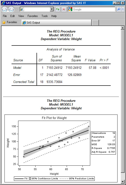
|
ods graphics on; ods select 'Analysis of Variance'; ods select 'Fit Plot'; proc reg data=sashelp.class; model weight=height; quit; ods graphics off; |
 |
1.3 What Is the SAS Graph Template Language (GTL)?
As mentioned in Section 1.1, GTL was originally designed to address the need to create complex graphs for SAS analytical procedures. Just as for tabular data, there was a need to display the data in a graphical form for easier understanding by the user. With SAS 9.2, the Output Delivery System (ODS) was extended to support graphics in a way similar to tabular data. The TEMPLATE procedure was extended to create STATGRAPH templates. These templates are defined using GTL, the syntax for graphs.
Another important feature of ODS Graphics is the systematic use of ODS styles for graphs. Each ODS destination has an associated default style, and all graphs and tables rendered to a destination use the attributes from the style to render themselves. The styles shipped with SAS are carefully designed to provide aesthetic output by default. You no longer have to tweak color and marker settings in the graphs to get great looking graphs from the system.
You can use the TEMPLATE procedure and GTL to create the STATGRAPH templates for your own custom graphs. GTL provides you an extensive set of plot types, layouts and other statements for legends, attribute maps etc. that you can use to define the graphs you need.
The automatic graphs produced by the SAS procedures mentioned in section 1.2 use the Graph Template Language (GTL) to create the graph. The structure of each graph is defined using the TEMPLATE procedure and GTL and stored in pre-defined STATGRAPH templates that are shipped with SAS. Each procedure then associates the run-time data with the appropriate pre-defined template to create the graphs.
In summary, the GTL syntax is the foundation of the ODS Graphics system and is used to define the structure of a graph. GTL is a flexible structured language that provides many features to define graphs from the simplest scatter plot to complex panels. This is the subject of this book.
1.4 Why Should You Learn GTL?
Here are some reasons to learn GTL.
• GTL provides in one system the full set of features that you need to create graphs from the simplest scatter plots to complex diagnostics panels.
• GTL is the language used to create the templates shipped by SAS for the creation of the automatic graphs from the analytical procedures. To customize one of these graphs, you will need to understand GTL.
• GTL represents the future for analytical graphics in SAS. New features are being added to GTL with every SAS release.
1.5 Making Graphs Using the Statistical Graphics (SG) Procedures
The SG procedures surface a simple procedure like syntax to create graphs using GTL under the covers. These are often all you need to create the graph that you want. These procedures are:
• The SGPLOT procedure for single-cell graphs
• The SGPANEL procedure for classification panel graphs
• The SGSCATTER procedure for comparative scatter plots and matrices
The details of the SG procedures can be found in the SAS documentation. For SAS 9.3 onwards, this is included in the Base SAS documentation. For earlier versions, it is included in the SAS/GRAPH documentation. A detailed description of the SG procedures is beyond the scope of this book.
If you prefer to create graphs using procedure syntax, the SG procedures may be the right tool for you. The book Statistical Graphics Procedures by Example – Effective Graphs Using SAS (Matange and Heath, 2011) provides a quick start to creating graphs using these procedures.
1.6 Making Graphs Using the ODS Graphics Designer
By far, the easiest and fastest way to create a custom graph is by using the ODS Graphics Designer, (referred to in this book as “Designer”). The interactive Designer application is the tool of choice for you if you fit the following profile:
• You want to create a graph quickly using an interactive application.
• You are not familiar with graph syntax, and have no desire to learn it.
• You export your data to third-party software just to create graphs.
Designer can help you create graphs with zero programming. Some key features are:
• Designer is an interactive GUI application.
• You can begin your graph from a gallery of commonly used graphs.
• You can customize your graph by adding more plots and insets.
• You can create single-cell graphs, classification panels, and ad hoc layouts.
• You can view the GTL code generated for you while creating the graph.
• You can save your custom graphs to the graph gallery for quick access.
• You can save your graph as a .sgd file to the file system.
• You can run a designer graph in batch using the SGDESIGN procedure to the open ODS destinations with the same or different data.
Designer is not only a great interactive tool to create your graph; it is also a great learning tool for GTL. You can see how the GTL is put together every time you make a change to the graph. You can copy the GTL code from the code window into the SAS program window and run the code.
1.7 Data Sets and Custom Styles Used in This Book
Most of the examples in this book use the data sets available in the SASHELP library. These include CARS, HEART, and a few others. Often, we need to subset the data set to reduce the number of classifiers or observations so that a graph will fit in the restricted space of the book. In other cases, custom data sets that are suitable for the example graph are needed.
Custom styles are sometimes used to render the graphs in this book. Primarily, these are necessary to reduce the font sizes to help fit the graphs into the small space available. This is especially true for examples of multi-cell graphs
Most graphs in this book from Chapter 4 onwards use the following settings:
ods listing image_dpi=300;
ods graphics / reset width=4in height=2.5in;
1.8 Color and Gray-scale Graphs
The graphs are created using the active style of the open destination. Often, these styles are optimized for full color output. This works well when the graph is also viewed in a color medium.
However, when color graphs are printed in gray scale, there is a significant loss of fidelity in the representation of distinct categories in the graph. For example, a graph with two series plots, one for Drug A and one for Drug B, can be well represented in color with the use of two distinct colors, such as red and blue. These colors are often designed to have equal weight to avoid unintentional bias.
When such a graph is printed in gray scale, these two series plots may look very similar unless they have other distinguishing features such as line patterns or marker shapes. Bar charts can benefit from the use of fill patterns to facilitate such discrimination.
This book is printed in gray scale, so it is important to create the graphs that will print legibly in a gray-scale format. When necessary, some graphs in this book are created using a gray-scale style such as Journal or styles derived from it.
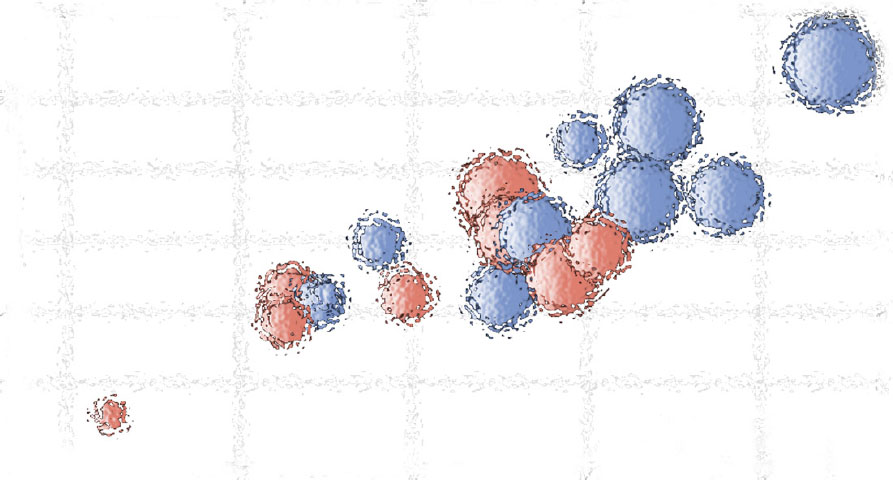
1.9 Effective Graphics and the Use of Decorative Skins
Graphs that are created by any of the methods mentioned above are built with the principles of effective graphics in mind as presented in Statistical Graphics Procedures by Example, 2011. By default, the system always strives to create a graph that delivers the information with maximum clarity and minimum clutter or distraction.
Though initially designed with the statistical user in mind, these graphs are finding increasing use in non-statistical domains. In such use cases, there is often a desire for a flashier graph, even at the expense of some effectiveness.
In SAS 9.2, only the Bar Chart statement(s) support decorative skins, and the option is undocumented. With SAS 9.3, options for skins are in production and have been documented. Also, new statement types have been added that are suited to “business” visualization, such as Pie Charts, Waterfall Charts, etc. With SAS 9.4, we go even further, and data skins are supported for almost all the plot types.
1.10 SAS 9.2, SAS 9.3, and SAS 9.4 Features
This book assumes that you have the SAS 9.2 (TS2M3) or higher release. The examples in this book include the use of SAS 9.2 (TS2M3), SAS 9.3, and SAS 9.4 features. Examples that use the features from SAS 9.4 are so marked.