Mathematical Thinking
Mathematics is both the queen and the handmaiden of all sciences—Eric Temple Bell.
It would be great if we could study the physical world unencumbered by the need for higher mathematics. This is probably the way it was for the ancient Greek natural philosophers. Nowadays, however, you can’t get very far in science or engineering without expressing results in mathematical language. This is not entirely a bad thing, since mathematics turns out to be more than just a language for science. It can also be an inspiration for conceptual models which provide deeper insights into natural phenomena. Indeed the essence of many physical laws is most readily apparent when they are expressed as mathematical equations—think of ![]() . As you go on, you will find that mathematics can provide indispensable short-cuts for solving complicated problems. Sometimes, mathematics is actually an alternative to thinking! At the very least, mathematics is one of the greatest labor-saving inventions ever created by Mankind.
. As you go on, you will find that mathematics can provide indispensable short-cuts for solving complicated problems. Sometimes, mathematics is actually an alternative to thinking! At the very least, mathematics is one of the greatest labor-saving inventions ever created by Mankind.
Instead of outlining some sort of “12-Step Program” for developing your mathematical skills, we will give 12 examples which will hopefully stimulate your imagination on how to think cleverly along mathematical lines. It will be worthwhile for you to study each example until you understand it completely and have internalized the line of reasoning. You might have to put off doing some of Examples 7–12 until you review some relevant calculus background in the later chapters of this book.
1.1 The NCAA March Madness Problem
Every March, according to a new format adopted in 2012, 68 college basketball teams are invited to compete in the NCAA tournament to determine a national champion. (Congratulations, 2012 Kentucky Wildcats!) Let’s calculate the total number of games that have to be played. First, 8 teams participate in 4 “play in” games to reduce the field to 64, a nice power of 2. In the first round, 32 games reduce the field to 32. In the second round, 16 games produce 16 winners who move on to 4 regional tournaments. There are then 8 games followed by 4 games to determine the “final 4.” The winner is then decided the following week by two semifinals followed by the championship game. If you’re keeping track, the total number of games to determine the champion equals ![]() . But there’s a much more elegant way to solve the problem. Since this is a single-elimination tournament, 67 of the 68 teams have to eventually lose a game. Therefore we must play exactly 67 games!
. But there’s a much more elegant way to solve the problem. Since this is a single-elimination tournament, 67 of the 68 teams have to eventually lose a game. Therefore we must play exactly 67 games!
1.2 Gauss and the Arithmetic Series
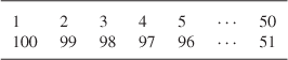
A tale in mathematical mythology—it’s hard to know how close it is to the actual truth—tells of Carl Friedrich Gauss as a 10-year-old student. By one account, Gauss’ math teacher wanted to take a break so he assigned a problem he thought would keep the class busy for an hour or so. The problem was to add up all the integers from 1 to 100. Supposedly, Gauss almost immediately wrote down the correct answer 5050 and sat with his hands folded for the rest of the hour. The rest of his classmates got incorrect answers! Here’s how he did it. Gauss noted that the 100 integers could be arranged into 50 pairs:
Each pair adds up to 101, thus the sum equals ![]() . The general result for the sum of an arithmetic progression with n terms is:
. The general result for the sum of an arithmetic progression with n terms is:
![]() (1.1)
(1.1)
where a and ![]() are the first and last terms, respectively. This holds true whatever the difference between successive terms.
are the first and last terms, respectively. This holds true whatever the difference between successive terms.
Problem 1.2.1
Evaluate the sum ![]() .
.
1.3 The Pythagorean Theorem
The most famous theorem in Euclidean geometry is usually credited to Pythagoras (ca. 500 BC). However, Babylonian tablets suggest that the result was known more than a thousand years earlier. The theorem states that the square of the hypotenuse c of a right triangle is equal to the sum of the squares of the lengths a and b of the other two sides:
![]() (1.2)
(1.2)
The geometrical significance of the Pythagorean theorem is shown in Figure 1.1: the sum of the areas of the red and the blue squares equals the area of the purple square.
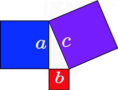
Figure 1.1 Geometrical interpretation of Pythagoras’ theorem. The purple area equals the sum of the blue and red areas. (For interpretation of the references to color in this figure legend, the reader is referred to the web version of this book.)
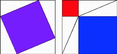
Well over 350 different proofs of the theorem have been published. Figure 1.2 shows a pictorial proof which requires neither words nor formulas.
1.4 Torus Area and Volume
A torus or anchor ring, drawn in Figure 1.3, is the approximate shape of a donut or bagel. The radii R and r refer, respectively, to the circle through the center of the torus and the circle made by a cross-sectional cut. Generally, to determine the area and volume of a surface of revolution, it is necessary to evaluate double or triple integrals. However, long before calculus was invented, Pappus of Alexandria (ca. 3rd Century AD) proposed two theorems which can give the same results much more directly.

The first theorem of Pappus states that the area A generated by the revolution of a curve about an external axis is equal to the product of the arc length of the generating curve and the distance traveled by the curve’s centroid. For a torus the generating curve is a small circle of radius r, which has an arc length of ![]() . The centroid is the center of the circle. In one revolution about the axis of the torus, the centroid travels a distance
. The centroid is the center of the circle. In one revolution about the axis of the torus, the centroid travels a distance ![]() . Therefore the surface area of a torus is
. Therefore the surface area of a torus is
![]() (1.3)
(1.3)
Similarly, the second theorem of Pappus states that the volume of the solid generated by the revolution of a figure about an external axis is equal to the product of the area of the figure and the distance traveled by its centroid. For a torus, the area of the cross-section equals ![]() . Therefore the volume of a torus is
. Therefore the volume of a torus is
![]() (1.4)
(1.4)
For less symmetrical figures, finding the centroid will usually require doing an integration.
An incidental factoid. You probably know about the four-color theorem: on a plane or spherical surface, four colors suffice to draw a map in such a way that regions sharing a common boundary have different colors. On the surface of a torus it takes seven colors.
Problem 1.4.1
Using the theorems of Pappus, calculate the volume and surface area of a flat cylindrical disk of width w, outer radius ![]() , and inner radius
, and inner radius ![]() . Check the results using the volume and area formulas for cylinders.
. Check the results using the volume and area formulas for cylinders.
1.5 Einstein’s Velocity Addition Law
Suppose a baseball team is traveling on a train moving at 60 mph. The star fastball pitcher needs to tune up his arm for the next day’s game. Fortunately one of the railroad cars is free and its full length is available. If his 90 mph pitches are in the same direction the train is moving, the ball will actually be moving at 150 mph relative to the ground. The law of addition of velocities in the same direction is relatively straightforward, ![]() . But according to Einstein’s special theory of relativity, this is only approximately true and requires that
. But according to Einstein’s special theory of relativity, this is only approximately true and requires that ![]() and
and ![]() be small fractions of the speed of light,
be small fractions of the speed of light, ![]() (or 186,000 miles/s). Expressed mathematically, we can write
(or 186,000 miles/s). Expressed mathematically, we can write
![]() (1.5)
(1.5)
According to special relativity, the speed of light, when viewed from any frame of reference, has the same constant value c. Thus, if an atom moving at velocity v emits a light photon at velocity c, the photon will still be observed to move at velocity c, not ![]() .
.
Our problem is to deduce the functional form of ![]() consistent with these facts. It is convenient to build in the known asymptotic behavior for
consistent with these facts. It is convenient to build in the known asymptotic behavior for ![]() by defining
by defining
![]() (1.6)
(1.6)
when ![]() , we evidently have
, we evidently have ![]() , so
, so
![]() (1.7)
(1.7)
and likewise
![]() (1.8)
(1.8)
If both ![]() and
and ![]() equal c,
equal c,
![]() (1.9)
(1.9)
A few moments’ reflection should convince you that a function consistent with these properties is
![]() (1.10)
(1.10)
We thus obtain Einstein’s velocity addition law:
![]() (1.11)
(1.11)
1.6 The Birthday Problem
It is a possibly surprising fact that if you have 23 people in your class or at a party, there is a better than 50% chance that two people share the same birthday (same month and day, not necessarily in the same year). Of course, we assume from the outset that there are no sets of twins or triplets present. There are 366 possible birthdays (including February 29 for leap years). For 367 people, at least two of them would be guaranteed to have the same birthday. But you have a good probability of a match with far fewer people. Each person in your group can have one of 366 possible birthdays. For two people, there are ![]() possibilities and for n people,
possibilities and for n people, ![]() possibilities. Now let’s calculate the number of ways that n people can have different birthdays. The first person can again have 366 possible birthdays, but the second person is now limited to the remaining 365 days, the third person to 364 days, and so forth. The total number of possibilities for no two birthdays coinciding is therefore equal to
possibilities. Now let’s calculate the number of ways that n people can have different birthdays. The first person can again have 366 possible birthdays, but the second person is now limited to the remaining 365 days, the third person to 364 days, and so forth. The total number of possibilities for no two birthdays coinciding is therefore equal to ![]() . In terms of factorials, this can be expressed
. In terms of factorials, this can be expressed ![]() . Dividing this number by
. Dividing this number by ![]() then gives the probability that no two people have the same birthday. Subtracting this from 1 gives the probability that this is not true, in other words, the probability that at least two people do have coinciding birthdays is given by
then gives the probability that no two people have the same birthday. Subtracting this from 1 gives the probability that this is not true, in other words, the probability that at least two people do have coinciding birthdays is given by
![]() (1.12)
(1.12)
Using your calculator, you will find that for ![]() . This means that there is a slightly better than 50% chance that 2 out of the 23 people will have the same birthday.
. This means that there is a slightly better than 50% chance that 2 out of the 23 people will have the same birthday.
1.7 Fibonacci Numbers and the Golden Ratio
The sequence of Fibonacci numbers is given by: ![]() , in which each number is the sum of the two preceding numbers. This can be expressed as
, in which each number is the sum of the two preceding numbers. This can be expressed as
![]() (1.13)
(1.13)
Fibonacci (whose real name was Leonardo Pisano) found this sequence as the number of pairs of rabbits n months after a single pair begins breeding, assuming that the rabbits produce offspring when they are two months old. As ![]() , the ratios of successive Fibonacci numbers
, the ratios of successive Fibonacci numbers ![]() approach a limit designated
approach a limit designated ![]() :
:
![]() (1.14)
(1.14)
which is equivalent to
![]() (1.15)
(1.15)
This implies the reciprocal relation
![]() (1.16)
(1.16)
Dividing Eq. (1.13) by ![]() , we obtain
, we obtain
![]() (1.17)
(1.17)
In the limit as ![]() this reduces to
this reduces to
![]() (1.18)
(1.18)
giving the quadratic equation
![]() (1.19)
(1.19)
with roots
![]() (1.20)
(1.20)
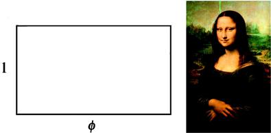
The positive root, ![]() , is known as the “golden ratio.” According to the ancient Greeks, this was supposed to represent the most esthetically pleasing proportions for a rectangle, as shown in Figure 1.4. Leonardo da Vinci also referred to it as the “divine proportion.”
, is known as the “golden ratio.” According to the ancient Greeks, this was supposed to represent the most esthetically pleasing proportions for a rectangle, as shown in Figure 1.4. Leonardo da Vinci also referred to it as the “divine proportion.”
Problem 1.7.1
Show that the golden ratio can be represented by the infinite sequence of nested square roots:
![]()
Calculate the approximate values of ![]() for 3, 4, and 5 square roots (and more if you use a programmable calculator or a computer program).
for 3, 4, and 5 square roots (and more if you use a programmable calculator or a computer program).
1.8  in the Gaussian Integral
![]() (1.21)
(1.21)
for the definite integral of a Gaussian function. The British mathematician J.E. Littlewood judged this remarkable result as “not accessible to intuition at all.” To derive Eq. (1.21), denote the integral by I and take its square:
![]() (1.22)
(1.22)
where the dummy variable y has been substituted for x in the last integral. The product of two integrals can be expressed as a double integral:
![]() (1.23)
(1.23)
The differential ![]() represents an element of area in Cartesian coordinates, with the domain of integration extending over the entire xy-plane. An alternative representation of the last integral can be expressed in plane polar coordinates
represents an element of area in Cartesian coordinates, with the domain of integration extending over the entire xy-plane. An alternative representation of the last integral can be expressed in plane polar coordinates ![]() . The two coordinate systems are related by
. The two coordinate systems are related by
![]() (1.24)
(1.24)
so that
![]() (1.25)
(1.25)
The element of area in polar coordinates is given by ![]() , so that the double integral becomes
, so that the double integral becomes
![]() (1.26)
(1.26)
Integration over ![]() gives a factor
gives a factor ![]() . The integral over r can be done after the substitution
. The integral over r can be done after the substitution ![]() :
:
![]() (1.27)
(1.27)
Therefore, ![]() and Laplace’s result (1.21) follows from the square root.
and Laplace’s result (1.21) follows from the square root.
Problem 1.8.1
Evaluate the integral ![]() .
.
Problem 1.8.2
Evaluate the integral ![]() , where
, where ![]() .
.
Problem 1.8.3
By taking the derivative with respect to ![]() of the above integral, evaluate
of the above integral, evaluate ![]() , where
, where ![]() .
.
1.9 Function Equal to Its Derivative
The problem is to find a function ![]() which is equal to its own derivative
which is equal to its own derivative ![]() . Assume that
. Assume that ![]() can be expressed as a power series
can be expressed as a power series
![]() (1.28)
(1.28)
Now differentiate term by term to get
![]() (1.29)
(1.29)
where the second sum is obtained by the replacement ![]() . Since
. Since ![]() , we can equate the corresponding coefficients of
, we can equate the corresponding coefficients of ![]() their expansions. This gives
their expansions. This gives
![]() (1.30)
(1.30)
or
![]() (1.31)
(1.31)
Specifically,
![]() (1.32)
(1.32)
The constant ![]() is most conveniently set equal to 1, and so
is most conveniently set equal to 1, and so
![]() (1.33)
(1.33)
Thus
![]() (1.34)
(1.34)
But this is just the well-known expansion for the exponential function, ![]() . The function is, as well, equal to its nth derivative:
. The function is, as well, equal to its nth derivative: ![]() , for all n.
, for all n.
A more direct way to solve the problem is to express it as a differential equation
![]() (1.35)
(1.35)
or
![]() (1.36)
(1.36)
This can be integrated to give
![]() (1.37)
(1.37)
The constant can most simply be chosen equal to zero. Exponentiating the last equation—that is, taking e to the power of each side—we find again
![]() (1.38)
(1.38)
1.10 Stirling’s Approximation for  !
!
Recall the definition of N factorial:
![]() (1.39)
(1.39)
Taking the natural logarithm, the product reduces to a sum:
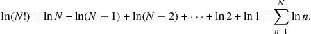 (1.40)
For large values of N, the sum over n can be well approximated by an integral over a continuous variable x:
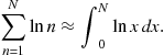 (1.41)
The precise choice of lower limit is unimportant since its contribution will be negligible compared to the upper limit. The integral of the natural log is given by
![]() (1.42)
(1.42)
which can be checked by taking the derivative. Therefore
![]() (1.43)
(1.43)
This result is the logarithmic version of Stirling’s approximation, which finds application in statistical mechanics.
The corresponding result for ![]() itself,
itself, ![]() , is much less accurate, since taking exponentials magnifies the error. A more advanced version of Stirling’s approximation is given by
, is much less accurate, since taking exponentials magnifies the error. A more advanced version of Stirling’s approximation is given by
![]() (1.44)
(1.44)
1.11 Potential and Kinetic Energies
This is really a topic in elementary mechanics, but it has the potential to increase your mathematical acuity as well. Let us start with the definition of work. If a constant force F applied to a particle moves it a distance x. The work done on the particle equals ![]() . If force varies with position, the work is given by an integral over x:
. If force varies with position, the work is given by an integral over x:
![]() (1.45)
(1.45)
For now, let us assume that the force and motion are exclusively in the x-direction. Now work has dimensions of energy and, more specifically, the energy imparted to the particle comes at the expense of the potential energy![]() possessed by the particle. We have therefore that
possessed by the particle. We have therefore that
![]() (1.46)
(1.46)
Expressed as its differential equivalent, this gives the relation between force and potential energy:
![]() (1.47)
(1.47)
The kinetic energy of a particle can be deduced from Newton’s second law
![]() (1.48)
(1.48)
where m is the mass of the particle and a, its acceleration. Acceleration is the time derivative of the velocity ![]() or the second time derivative of the position x. In the absence of friction and other nonconservative forces, the work done on a particle, considered above, serves to increase its kinetic energy T—the energy a particle possesses by virtue of its motion. By the conservation of energy,
or the second time derivative of the position x. In the absence of friction and other nonconservative forces, the work done on a particle, considered above, serves to increase its kinetic energy T—the energy a particle possesses by virtue of its motion. By the conservation of energy,
![]() (1.49)
(1.49)
The time derivatives of the energy components must therefore obey
![]() (1.50)
(1.50)
From the differential relation for work
![]() (1.51)
(1.51)
we obtain the work done per unit time, known as the power
![]() (1.52)
(1.52)
Therefore, using Newton’s second law
![]() (1.53)
(1.53)
If we choose the constant of integration such that ![]() when
when ![]() , we obtain the well-known equation for the kinetic energy of a particle:
, we obtain the well-known equation for the kinetic energy of a particle:
![]() (1.54)
(1.54)
Generalizing the preceding formulas to three dimensions, work would be represented by a line integral
![]() (1.55)
(1.55)
and the force would equal the negative gradient of the potential energy
![]() (1.56)
(1.56)
In three-dimensional vector form, Newton’s second law becomes
![]() (1.57)
(1.57)
The kinetic energy would still work out to ![]() but now
but now
![]() (1.58)
(1.58)
Our derivation of the kinetic energy is valid in the nonrelativistic limit when ![]() , the speed of light. Einstein’s more general relation for the energy of a particle of mass m moving at speed
, the speed of light. Einstein’s more general relation for the energy of a particle of mass m moving at speed ![]() (in the absence of potential energy) is
(in the absence of potential energy) is
![]() (1.59)
(1.59)
For ![]() , the square root can be expanded using the binomial theorem to give
, the square root can be expanded using the binomial theorem to give
![]() (1.60)
(1.60)
The first term represents the rest energy of the particle—the energy equivalence of mass first understood by Einstein—while the second term reproduces our result for kinetic energy.
Problem 1.11.1
The force on a mass attached to a spring of force constant k is approximated by Hooke’s law, ![]() , where x is the displacement of the spring from its equilibrium length. Derive an expression for the potential energy
, where x is the displacement of the spring from its equilibrium length. Derive an expression for the potential energy ![]() .
.
1.12 Riemann Zeta Function and Prime Numbers
This last example is rather difficult but will really sharpen your mathematical wits if you can master it (don’t worry if you can’t).
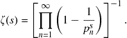
The Riemann zeta function is defined by
![]() (1.61)
(1.61)
The function is finite for all values of s in the complex plane except for the point ![]() . Euler in 1737 proved a remarkable connection between the zeta function and an infinite product containing the prime numbers:
. Euler in 1737 proved a remarkable connection between the zeta function and an infinite product containing the prime numbers:
 (1.62)
The product notation ![]() is analogous to
is analogous to ![]() for sums. More explicitly,
for sums. More explicitly,
![]() (1.63)
(1.63)
Thus
![]() (1.64)
(1.64)
where ![]() runs over all the prime numbers 2, 3, 5, 7, 11, …
runs over all the prime numbers 2, 3, 5, 7, 11, …
To prove the result, consider first the product
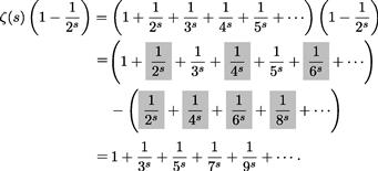 (1.65).
The shaded terms cancel out. Multiplying by the factor ![]() has evidently removed all the terms divisible by 2 from the zeta function series. The next step is to multiply by
has evidently removed all the terms divisible by 2 from the zeta function series. The next step is to multiply by ![]() . This gives
. This gives

Continuing the process, we successively remove all remaining terms containing multiples of 5, 7, 11, etc. Finally, we obtain
![]() (1.67)
(1.67)
which completes the proof of Euler’s result.
1.13 How to Solve It
Although we had promised not to give you any mathematical “good advice” in abstract terms, the book by George Polya, How to Solve It (Princeton University Press, 1973), contains a procedural approach to problem solving which can be useful sometimes. The following summary is lifted verbatim from the book’s preface.
1.13.1 Understanding the Problem
First. You have to understand the problem. What is the unknown? What are the data? What is the condition? Is it possible to satisfy the condition? Is the condition sufficient to determine the unknown? Or is it insufficient? Or redundant? Or contradictory? Draw a figure. Introduce suitable notation. Separate the various parts of the condition. Can you write them down?
1.13.2 Devising a Plan
Second. Find the connection between the data and the unknown. You may be obliged to consider auxiliary problems if an immediate connection cannot be found. You should obtain eventually a plan of the solution. Have you seen it before? Or have you seen the same problem in a slightly different form? Do you know a related problem? Do you know a theorem that could be useful? Look at the unknown! And try to think of a familiar problem having the same or a similar unknown. Here is a problem related to yours and solved before. Could you use it? Could you use its result? Could you use its method? Should you introduce some auxiliary element in order to make its use possible? Could you restate the problem? Could you restate it still differently? Go back to definitions. If you cannot solve the proposed problem try to solve first some related problem. Could you imagine a more accessible related problem? A more general problem? A more special problem? An analogous problem? Could you solve a part of the problem? Keep only a part of the condition, drop the other part; how far is the unknown then determined, how can it vary? Could you derive something useful from the data? Could you think of other data appropriate to determine the unknown? Could you change the unknown or data, or both if necessary, so that the new unknown and the new data are nearer to each other? Did you use all the data? Did you use the whole condition? Have you taken into account all essential notions involved in the problem?
1.13.3 Carrying Out the Plan
Third. Carry out your plan. Carrying out your plan of the solution, check each step. Can you see clearly that the step is correct? Can you prove that it is correct?
1.13.4 Looking Back
Fourth. Examine the solution obtained. Can you check the result? Can you check the argument? Can you derive the solution differently? Can you see it at a glance? Can you use the result, or the method, for some other problem?
1.14 A Note on Mathematical Rigor
Actually, the absence thereof. If any real mathematician should somehow come across this book, he or she will quickly recognize that it has been produced by Nonunion Labor. While I have tried very hard not to say anything grossly incorrect, I have played fast and loose with mathematical rigor. For the intended reading audience, I have made use of reasoning on a predominantly intuitive level. I am usually satisfied with making a mathematical result you need at least plausible, without always providing a rigorous proof. In essence, I am providing you with a lifeboat, not a luxury liner. Nevertheless, as you will see, I am not totally insensitive to mathematical beauty.
As a biologist, a physicist, and a mathematician were riding on a train moving through the countryside, all see a brown cow. The biologist innocently remarks: “I see cows are brown.” The physicist corrects him: “That’s too broad a generalization, you mean some cows are brown.” Finally, the mathematician provides the definitive analysis: “There exists at least one cow, one side of which is brown.”
The great physicist Hans Bethe believed in utilizing minimal mathematical complexity to solve physical problems. According to his long-time colleague E.E. Salpeter, “In his hands, approximations were not a loss of elegance but a device to bring out the basic simplicity and beauty of each field.” One of our recurrent themes will be to formulate mathematical problems in a way which leads to the most transparent and direct solution, even if this has to be done at the expense of some rigor.
As the mathematician and computer scientist Richard W. Hamming opined, “Does anyone believe that the difference between the Lebesgue and Riemann integrals can have physical significance, and that whether, say, an airplane would or would not fly could depend on this difference? If such were claimed, I should not care to fly in that plane.” Riemann integrals are the only type we will encounter in this book. Lebesgue integrals represent a generalization of the concept, which can deal with a larger class of functions, including those with an infinite number of discontinuities.
A somewhat irreverent spoof of how a real mathematician might rigorously express the observation “Suzy washed her face” might run as follows. Let there exist a ![]() such that the image of
such that the image of ![]() of the point
of the point ![]() under the bijective mapping
under the bijective mapping ![]() belongs to the set
belongs to the set ![]() of girls with dirty faces and let there exist a
of girls with dirty faces and let there exist a ![]() in the half-open interval
in the half-open interval ![]() such that the image of the point
such that the image of the point ![]() under the same mapping belongs to
under the same mapping belongs to ![]() , the complement of
, the complement of ![]() , with respect to the initial point
, with respect to the initial point ![]() .
.
Just in case we have missed offending any reader, let us close with a quote from David Wells, The Penguin Dictionary of Curious and Interesting Numbers (Penguin Books, Middlesex, England, 1986):
Mathematicians have always considered themselves superior to physicists and, of course engineers. A mathematician gave this advice to his students: “If you can understand a theorem and you can prove it, publish it in a mathematics journal. If you understand it but can’t prove it, submit it to a physics journal. If you can neither understand it nor prove it, send it to a journal of engineering.”