The SVM method is a set of algorithms used for classification and regression analysis tasks. Considering that in an N-dimensional space, each object belongs to one of two classes, SVM generates an (N-1)-dimensional hyperplane to divide these points into two groups. It's similar to an on-paper depiction of points of two different types that can be linearly divided. Furthermore, the SVM selects the hyperplane, which is characterized by the maximum distance from the nearest group elements.

The input data can be separated using various hyperplanes. The best hyperplane is a hyperplane with the maximum resulting separation and the maximum resulting difference between the two classes.

Imagine the data points on the plane. In the following case, the separator is just a straight line:

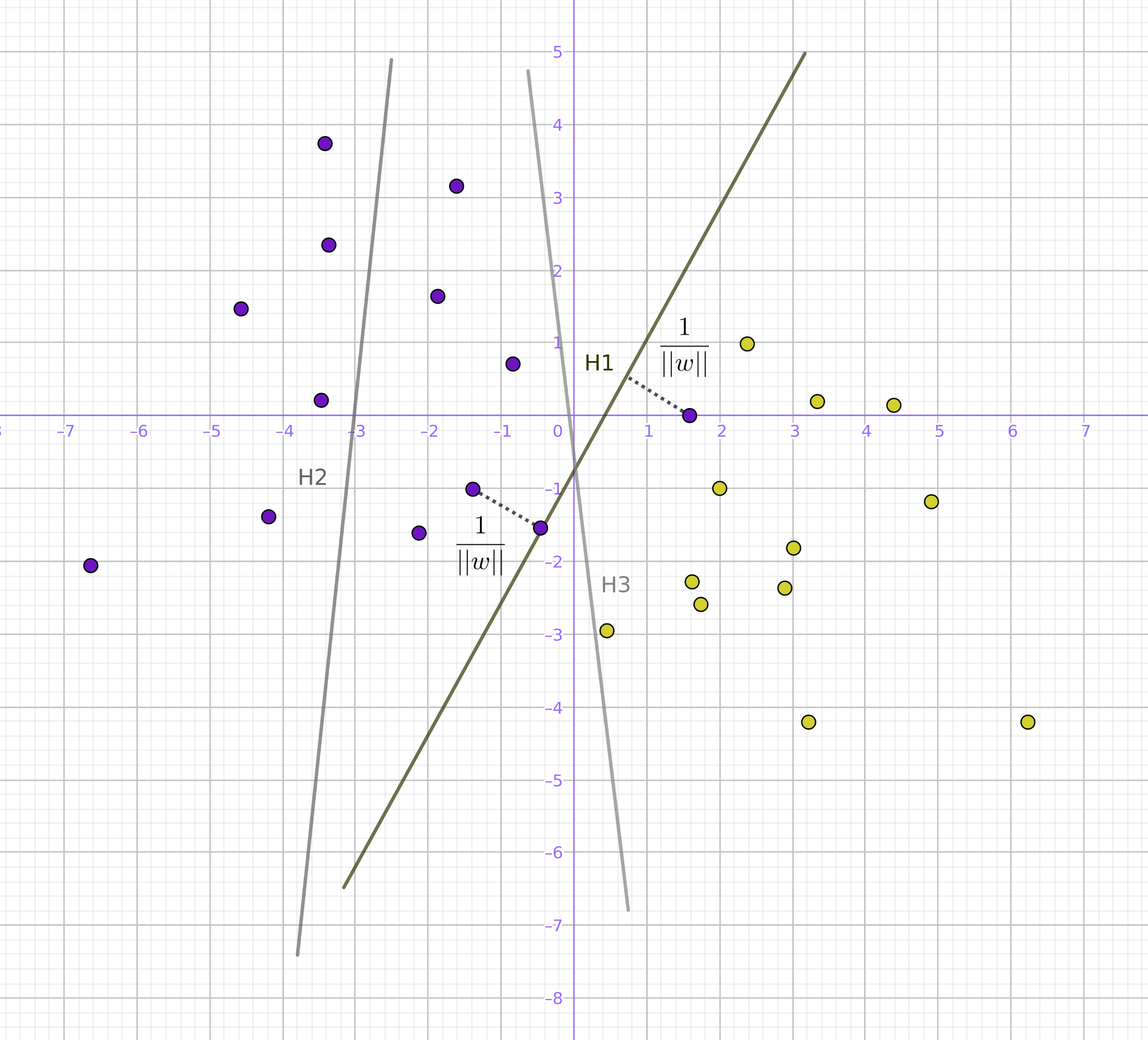
Let's draw distinct straight lines that divide the points into two sets. Then, choose a straight line as far as possible from the points, maximizing the distance from it to the nearest point on each side. If such a line exists, then it is called the maximum margin hyperplane. Intuitively, a good separation is achieved due to the hyperplane itself (which has the longest distance to the nearest point of the training sample of any class), since, in general, the bigger the distance, the smaller the classifier error.

Consider learning samples given with the set consisting of objects with parameters, where takes the values -1 or 1, therefore defining the point's classes. Each point is a vector of the dimension . Our task is to find the maximum margin hyperplane that separates the observations. We can use analytic geometry to define any hyperplane as a set of points that satisfy the condition, as illustrated here:

Here,  and .

Thus, the linear separating (discriminant) function is described by the equation g(x)=0. The distance from the point to the separating function g(x)=0 (the distance from the point to the plane) is equal to the following:

lies in the closure of the boundary that is . The border, which is the width of the dividing strip, needs to be as large as possible. Considering that the closure of the boundary satisfies the condition , then the distance from is as follows:

Thus, the width of the dividing strip is . To exclude points from the dividing strip, we can write out the following conditions:

Let's also introduce the index function that shows to which class  belongs, as follows:

Thus, the task of choosing a separating function that generates a corridor of the greatest width can be written as follows:

The J(w) function was introduced with the assumption that for all . Since the objective function is quadratic, this problem has a unique solution.

According to the Kuhn-Tucker theorem, this condition is equivalent to the following problem:

This is provided that and , where , are new variables. We can rewrite in the matrix form, as follows:

The H coefficients of the matrix can be calculated as follows: $. Quadratic programming methods can solve the task .

After finding the optimal for every , one of the two following conditions is fulfilled:

1.  (i corresponds to a non-support vector.)
2.  (i corresponds to a support vector.)

Then,  can be found from the relation , and the value of can be determined, considering that for any and , as follows:

Finally, we can obtain the discriminant function, illustrated here:

Note that the summation is not carried out over all vectors, but only over the set S, which is the set of support vectors .

Unfortunately, the described algorithm is realized only for linearly separable datasets, which in itself occurs rather infrequently. There are two approaches for working with linearly non-separable data.

One of them is called a soft margin, which chooses a hyperplane that divides the training sample as purely (with minimal error) as possible, while at the same time maximizing the distance to the nearest point on the training dataset. For this, we have to introduce additional variables , which characterize the magnitude of the error on each object x_i. Furthermore, we can introduce the penalty for the total error into the goal functional, like this:

Here,  is a method tuning parameter that allows you to adjust the relationship between maximizing the width of the dividing strip and minimizing the total error. The value of the penalty for the corresponding object x_i depends on the location of the object x_i relative to the dividing line. So, if x_i lies on the opposite side of the discriminant function, then we can assume the value of the penalty , if x_i lies in the dividing strip, and comes from its class. The corresponding weight is, therefore, . In the ideal case, we assume that . The resulting problem can then be rewritten as follows:

Notice that elements that are not an ideal case are involved in the minimization process too, as illustrated here:

Here, the constant β is the weight that takes into account the width of the strip. If β is small, then we can allow the algorithm to locate a relatively high number of elements in a non-ideal position (in the dividing strip). If β is vast, then we require the presence of a small number of elements in a non-ideal position (in the dividing strip). Unfortunately, the minimization problem is rather complicated due to the discontinuity. Instead, we can use the minimization of the following:

This occurs under restrictions , as illustrated here:

Another idea of ​​the SVM method in the case of the impossibility of a linear separation of classes is the transition to a space of higher dimension, in which such a separation is possible. While the original problem can be formulated in a finite-dimensional space, it often happens that the samples for discrimination are not linearly separable in this space. Therefore, it is suggested to map the original finite-dimensional space into a larger dimension space, which makes the separation much easier. To keep the computational load reasonable, the mappings used in support vector algorithms provide ease of calculating points in terms of variables in the original space, specifically in terms of the kernel function.

First, the function of the mapping  is selected to map the data of into a space of a higher dimension. Then, a non-linear discriminant function can be written in the form . The idea of ​​the method is to find the kernel function and maximize the objective function, as illustrated here:

Here, to minimize computations, the direct mapping of data into a space of a higher dimension is not used. Instead, an approach called the kernel trick (see Chapter 6, Dimensionality Reduction) is used—that is, K(x, y), which is a kernel matrix.

In general, the more support vectors the method chooses, the better it generalizes. Any training example that does not constitute a support vector is correctly classified if it appears in the test set because the border between positive and negative examples is still in the same place. Therefore, the expected error rate of the support vector method is, as a rule, equal to the proportion of examples that are support vectors. As the number of measurements grows, this proportion also grows, so the method is not immune from the curse of dimensionality, but it is more resistant to it than most algorithms.
It is also worth noting that the support vector method is sensitive to noise and data standardization.

Also, the method of SVMs is not only limited to the classification task but can also be adapted for solving regression tasks too. So, you can usually use the same SVM software implementation for solving classification and regression tasks.