4

Exploring Monte Carlo Simulations

Monte Carlo simulation is used to reproduce and numerically solve a problem in which random variables are also involved, and whose solution by analytical methods is too complex or impossible. In addition, the use of simulation allows you to test the effects of changes in the input variables or the output function more easily and with a high degree of detail. Starting from modeling the processes and generating random variables, simulations composed of multiple runs capable of obtaining an approximation of the probability of certain results are performed.

This method has assumed great importance in many scientific and engineering areas, above all for its ability to deal with complex problems that previously could only be solved through deterministic simplifications. It is mainly used in three distinct classes of problems: optimization, numerical integration, and generating probability functions. In this chapter, we will explore various techniques based on Monte Carlo methods for process simulation. First, we will learn about the basic concepts and then learn how to apply them to practical cases.

In this chapter, we’re going to cover the following main topics:

• Introducing the Monte Carlo simulation
• Understanding the central limit theorem
• Applying the Monte Carlo simulation
• Performing numerical integration using Monte Carlo
• Exploring sensitivity analysis concepts
• Explaining the cross-entropy method

Technical requirements

In this chapter, we will provide an introduction to Monte Carlo simulation. To deal with the topics in this chapter, it is necessary to have a basic knowledge of algebra and mathematical modeling.

To work with the Python code in this chapter, you’ll need the following files (available on GitHub at the following URL: https://github.com/PacktPublishing/Hands-On-Simulation-Modeling-with-Python-Second-Edition):

• simulating_pi.py
• central_limit_theorem.py
• numerical_integration.py
• sensitivity_analysis.py
• cross_entropy.py
• cross_entropy_loss_function.py

Introducing the Monte Carlo simulation

In simulation procedures, the evolution of a process is followed, but at the same time, forecasts of possible future scenarios are made. A simulation process consists of building a model that closely imitates a system. From the model, numerous samples of possible cases are generated and subsequently studied over time. After this, the results are analyzed over time, all while highlighting the alternative decisions that can be made.

The term Monte Carlo simulation was born at the beginning of the Second World War by J. von Neumann and S. Ulam as part of the Manhattan project at the Los Alamos nuclear research center. They replaced the parameters of the equations that describe the dynamics of nuclear explosions with a set of random numbers. The choice of the name Monte Carlo was due to the uncertainty of the winnings that characterize the famous casino of the Principality of Monaco.

Monte Carlo components

To obtain a simulation with satisfactory results, applications that use the Monte Carlo method are based on the following components:

• Probability density functions (PDFs) of the physical system
• Methods for estimating and reducing statistical error
• A uniform random number generator that allows us to obtain a uniform function distributed in a range between [0.1]
• An inversion function that allows one random uniform variable to be passed to a population variable
• Sampling rules so that we can divide the space into specific volumes of interest
• Parallelization and optimization algorithms for efficiently implementing the available computing architecture

The Monte Carlo simulation calculates a series of possible realizations of the phenomenon in question, along with the weight of the probability of a specific occurrence, while trying to explore the whole space of the parameters of the phenomenon.

Once this random sample has been calculated, the simulation gathers measurements of the quantities of interest in the sample. It is well executed if the average value of these measurements on the system realizations converges to the true value.

Important note

The functionality of Monte Carlo simulation can be summarized as follows: a phenomenon is observed n times, recording the methods adopted in each event, to identify the statistical distribution of the character.

First Monte Carlo application

The primary objective of the Monte Carlo method is to estimate a parameter that’s representative of a population. To do this, the calculator generates a series of n random numbers that make up the sample of the population in question.

For example, suppose we want to evaluate a parameter, A, that’s currently unknown, which can be interpreted as the average value of a random variable. The Monte Carlo method consists of, in this case, estimating this parameter by calculating the average of a sample consisting of N values of X. This is obtained using a procedure that involves the use of random numbers, as shown in the following diagram:

Figure 4.1 – Process of a random generator

In the Monte Carlo simulation, a series of possible realizations of a phenomenon are calculated to explore all the available parameters.

Important note

In this calculation, the weight of the probability of each event assumes importance. When the representative sample is calculated, the simulation measures the quantities of interest in this sample.

Monte Carlo simulation works if the average value of these measurements on the system converges to the real value.

Monte Carlo applications

The Monte Carlo simulation proves to be a valid tool for addressing the following problems:

• Intrinsically probabilistic problems involving phenomena related to the stochastic fluctuation of random variables
• Problems of an essentially deterministic nature, completely devoid of random components, but whose solution strategy can be treated as an expectation value of a function of stochastic variables

The necessary conditions to apply the method are the independence and analogy of the experiments. For independence, it is understood that the results of each repetition of the experiment must not be able to influence each other. By analogy, however, reference is made to the fact that, when observing the character, the same experiment is repeated n times.

Applying the Monte Carlo method for Pi estimation

The Monte Carlo method is a problem-solving strategy that uses statistics. If we use P to indicate the probability of a certain event, then we can randomly simulate this event and obtain P by making the ratio between the number of times our event occurred and the number of total simulations, as follows:

We can apply this strategy to get an approximation of Pi. Pi (π) is a mathematical constant indicating the relationship between the circumference of a circle and its diameter. If we denote the length of a circumference with C and its diameter with d, we know that C = d * π. The circumference of a circle with a diameter equal to 1 is π.

Important note

Usually, we approximate the value of Pi with 3.14 to simplify the accounts. However, π is an irrational number; that is, it has an infinite number of digits after the decimal point that never repeats regularly.

Given that a circle has a radius of 1, it can be inscribed in a square with a side equal to 2. For convenience, we will only consider a fraction of the circle, as shown in the following figure:

Figure 4.2 – A fraction of the circle

By analyzing the previous figure, we can see that the area of the square in blue is 1 and that the area of the circular sector in yellow (1/4 of the circle) is Pi/4. We randomly place a very large number of points inside the square. Thanks to the very large number and random distribution, we can approximate the size of the areas with the number of points contained in them.

If we generate N random numbers inside the square as the number of points that fall in the circular sector, which we will denote with M, divided by the total number of generated numbers, N, we will have to approximate the area of the circular sector, in which case it will be equal to Pi/4. From this, we can derive the following equation:

The greater the number of points generated, the more precise the approximation of Pi will be.

Now, let’s analyze the code line by line to understand how we have implemented the simulation procedure for estimating Pi:

1. To start, we import the necessary libraries:

   import math

   import random

   import numpy as np

   import matplotlib.pyplot as plt

The math library provides access to the mathematical functions defined by the C standard library. The random library implements pseudo-random number generators for various distributions. The random module is based on the Mersenne Twister algorithm. The numpy library offers additional scientific functions of the Python language, designed to perform operations on vectors and dimensional matrices. Finally, the matplotlib library is a Python library for printing high-quality graphics.

2. Let’s move on and initialize the parameters:

   N = 10000

   M = 0

As we mentioned previously, N represents the number of points that we generate – that is, those that we are going to position. Instead, M will be the points that fall within the circular sector. To start, these points will be zero and as we generate them, we will try to perform a check. In a positive scenario, we will gradually increase this number.

3. Let’s proceed and initialize the vectors that will contain the coordinates of the points that we will generate:

   XCircle=[]  

   YCircle=[]  

   XSquare=[]  

   YSquare=[]  

Here, we have defined two types of points: Circle and Square. Circle is a point that falls within the circular sector, while Square is a point that falls within the space of the square outside the circular sector. Now, we can generate the points:

for p in range(N):
    x=random.random()
    y=random.random()

Here, we used a for loop that iterates the process several times equal to the number, N, of samples we want to generate. Then, we used the random() function of the random library to generate the points. The random() function returns the next nearest floating-point value from the generated sequence. All the return values fall between 0 and 1.0.

4. Now, we can check where the point we just generated falls:

   if(x**2+y**2 <= 1):

           M+=1

           XCircle.append(x)  

           YCircle.append(y)        

       else:

           XSquare.append(x)  

           YSquare.append(y)

The if loop allows us to check the position of the points. Recall that the points of a circumference are defined by the following equation:

If x0=y0=0 and r=1, the previous equation turns into the following:

This makes us understand that the necessary condition for a point to fall within the circular sector is that the following equation is verified:

If this condition is satisfied, the value of M is increased by 1 unit and the values of the x and y values that are generated are stored in the Circle point vector (XCircle, YCircle). Otherwise, the value of M is not updated, and the values of x and y that are generated are stored in the vector of the Square point vector (XSquare, YSquare).

5. Now that we’ve iterated this procedure for the 10,000 points that we have decided to generate, we can estimate Pi:

   Pi = 4*M/N

   print("N=%d M=%d Pi=%.2f" %(N,M,Pi))

In this way, we can calculate Pi and print the results, as follows:

N=10000 M=7857 Pi=3.14

The estimate that we’ve obtained is acceptable. Usually, we stop at the second decimal place, so this is okay. Now, let’s draw a graph, where we will draw the generated points. To start, we will generate the points of the circumference arc:

XLin=np.linspace(0,1)
YLin=[]
for x in XLin:
    YLin.append(math.sqrt(1-x**2))

The linspace() function of the numpy library allows us to define an array composed of a series of N numerical elements equally distributed between two extremes (0,1). This will be the x of the arc of the circumference (XLin). On the other hand, the y numerical elements (YLin) will be obtained from the equation of the circumference while solving them concerning y, as follows:

To calculate the square root, we used the math.sqrt() function.

6. Now that we have all the points, we can draw the graph:

   plt.axis   ("equal")                             

   plt.grid   (which="major")                        

   plt.plot   (XLin , YLin, color="red" , linewidth="4") 

   plt.scatter(XCircle, YCircle, color="yellow", marker   =".") 

   plt.scatter(XSquare, YSquare, color="blue"  , marker   =".") 

   plt.title  ("Monte Carlo method for Pi estimation")

   plt.show()

The scatter() function allows us to represent a series of points not closely related to each other on two axes. The following diagram is printed:

Figure 4.3 – Plot of the Pi estimation

Consistent with what we established at the beginning of this chapter, we plotted the points inside the circular sector in yellow, while those outside the circular sector are in blue. To highlight the separation line, we have drawn the circumference arc in red.

Now that we’ve applied the Monte Carlo method to estimate Pi, the time has come to deepen some fundamental concepts for simulation based on generating random numbers.

Understanding the central limit theorem

The Monte Carlo method is essentially a numerical method for calculating the expected value of random variables; that is, an expected value that cannot be easily obtained through direct calculation. To obtain this result, the Monte Carlo method is based on two fundamental theorems of statistics: the law of large numbers and the central limit theorem.

Law of large numbers

This theorem states the following: considering a very large number of variables, ? (? → ∞), the integral that defines the average value is approximate to the estimate of the expected value. Let’s try to give an example so that you can understand this. We flip a coin 10 times, 100 times, and 1,000 times and check how many times we get heads. We can put the results we obtained into a table, as follows:

Table 4.1 – Table showing the results for a coin toss

Analyzing the last column of the previous table, we can see that the value of the frequency approaches that of the probability (50%). Therefore, we can say that as the number of tests increases, the frequency value tends to the theoretical probability value. The latter value can be achieved using the hypothesis of several throws that tend to infinity.

Important note

The use of the law of large numbers is different. The law of large numbers allowed us, in the Monte Carlo method for Pi estimation section, to equal the number of launches with the area of the circular sector. In this way, we were able to estimate the value of Pi simply by generating random numbers. Also, in this case, the greater the number of random variables generated, the closer the estimate of Pi is to the expected value.

The law of large numbers allows you to determine the centers and weights of a Monte Carlo analysis to estimate definite integrals but does not say how large the number, N, must be. You do not have an estimate to understand with what order of magnitude you can perform a simulation so that you can consider the numbers large enough. To answer this question, it is necessary to resort to the central limit theorem.

The central limit theorem

Monte Carlo not only allows us to obtain an estimate of the expected value, as established by the law of large numbers, but also allows us to estimate the uncertainty associated with it. This is possible thanks to the central limit theorem, which returns an estimate of the expected value and the reliability of that result.

Important note

The central limit theorem can be summarized with the following definition: given a dataset with an unknown distribution, the sample’s mean will approximate the normal distribution.

If the law of large numbers tells us that the random variable allows us to evaluate the expected value, the central limit theorem provides information on its distribution.

An interesting feature of the central limit theorem is that there are no constraints on the distribution of the function that’s used to generate the N samples from which the random variable is formed. It is not important what the distribution associated with the random variable is, but when the average is characterized by a finite variance and is obtained for a very large number of samples, it can be described through a Gaussian distribution.

Let’s take a look at a practical example. We generate 10,000 random numbers with a uniform distribution. Then, we extract 100 samples from this population, also taken randomly. We repeat this operation a consistent number of times and for each time, we evaluate its average and store this value in a vector. In the end, we draw a histogram of the distribution that we have obtained. Here is the Python code:

import random
import numpy as np
import matplotlib.pyplot as plt
a=1
b=100
N=10000  
DataPop=list(np.random.uniform(a,b,N))
plt.hist(DataPop, density=True, histtype='stepfilled', alpha=0.2)
plt.show()
SamplesMeans = []
for i in range(0,1000):
    DataExtracted = random.sample(DataPop,k=100)
    DataExtractedMean = np.mean(DataExtracted)
    SamplesMeans.append(DataExtractedMean)
plt.figure()
plt.hist(SamplesMeans, density=True, histtype='stepfilled', alpha=0.2)
plt.show()

Now, let’s analyze the code line by line to understand how we have implemented the simulation procedure to understand the central limit theorem:

1. To start, we import the necessary libraries:

   import random

   import numpy as np

   import matplotlib.pyplot as plt

The random library implements pseudo-random number generators for various distributions. The numpy library offers additional scientific functions of the Python language and is designed to perform operations on vectors and dimensional matrices.

Finally, the matplotlib library is a Python library for printing high-quality graphics.

2. Let’s move on and initialize the parameters:

   a=1

   b=100

   N=10000  

The a and b parameters are the extremes of the range, and N is the number of values we want to generate.

Now, we can generate the uniform distribution using the NumPy random.uniform() function, as follows:

 DataPop=list(np.random.uniform(a,b,N))

3. At this point, we draw a histogram of the data to verify that it is a uniform distribution:

   plt.hist(DataPop, density=True, histtype='stepfilled', alpha=0.2)

   plt.show()

The matplotlib.hist() function draws a histogram; that is, a diagram in classes of a continuous character.

This is used in many contexts, usually to show statistical data when there is an interval of the definition of the independent variable divided into subintervals.

The following diagram is printed:

Figure 4.4 – Plot of the data distribution

The distribution appears to be uniform – we can see that each bin is populated with an almost constant frequency.

4. Now, let’s pass the values to the extraction of the samples from the generated population:

   SamplesMeans = []

   for i in range(0,1000):

       DataExtracted = random.sample(DataPop,k=100)

       DataExtractedMean = np.mean(DataExtracted)

       SamplesMeans.append(DataExtractedMean)

First, we initialized the vector that will contain the samples. To do this, we used a for loop to repeat the operations 1,000 times. At each step, we extracted 100 samples from the population generated using the random.sample() function. The random.sample() function extracts samples without repeating the values and without changing the input sequence.

5. Next, we calculated the average of the extracted samples and added the result to the end of the vector containing the samples. Now, all we need to do is view the results:

   plt.figure()

   plt.hist(SamplesMeans, density=True, histtype='stepfilled', alpha=0.2)

   plt.show()

The following histogram is printed:

Figure 4.5 – Plot of the extracted samples

The distribution has now taken on the typical bell-shaped curve characteristic of the Gaussian distribution. This means that we have proved the central limit theorem.

Now, we are ready to apply the newly learned Monte Carlo simulation concepts to real cases.

Applying the Monte Carlo simulation

Monte Carlo simulation is used to study the response of a model that’s used randomly generated inputs. The simulation process takes place in the following three phases:

1. N inputs are generated randomly.
2. A simulation is performed for each of the N inputs.
3. The outputs of the simulations are aggregated and examined. The most common measures include estimating the average value of a certain output and distributing the output values, as well as the minimum or maximum output value.

Monte Carlo simulation is widely used for analyzing financial, physical, and mathematical models.

Generating probability distributions

Generating probability distributions that cannot be found with analytical methods can easily be addressed with Monte Carlo methods. For example, let’s say we want to estimate the probability distribution of the damage caused by earthquakes in a year in Japan.

Important note

In this type of analysis, there are two sources of uncertainty: how many earthquakes there will be in a year and how much damage each earthquake will do. Even if it is possible to assign a probability distribution to these two logical levels, it is not always possible to put this information together with analytical methods to derive the distribution of the annual losses.

It is easier to do a Monte Carlo simulation of this type like so:

1. A random number is extracted from the distribution of the number of annual events.
2. If events occur from the previous point, extractions are made from the distribution of losses.
3. Finally, we add the values of the extractions we performed to obtain a value that represents an annual loss caused by events.

By cyclically repeating these three points, a sample of annual losses is generated, from which it is possible to estimate the probability distribution that could not be obtained analytically.

Numerical optimization

Various algorithms can be used to find the local minima of a function. Typically, these algorithms proceed according to the following steps:

1. Start from an assigned point.
2. They control in which direction the function tends to have values smaller than the current one.
3. Moving in this direction, they find a new point where the function has a lower value than the previous one.

They keep repeating these steps until they reach a minimum. In the case of a function with only one minimum, this method allows us to achieve a result. But what if we have a function with many local minima and we want to find the point that minimizes the function globally? The following diagram shows the two cases just mentioned; that is, a distribution with only one minimum (left) and a distribution with several minimums (right):

Figure 4.6 – Graphs of the two distributions

A local search algorithm could stop at any of the many local minima of the function. How would you know if you found one of the many local minimums or the global minimum? There is no way to strictly establish this. The only practical possibility is to explore different areas of the search domain to increase the probability of finding, among the various local minima, the global one.

Important note

Different methods have been developed to explore domains that can be very complicated, with many dimensions and with constraints to be respected.

Monte Carlo methods provide a solution to this problem; that is, an initial population of points belonging to the domain is created, which is then evolved by defining coupling algorithms between the points in which random genetic mutations also occur. When simulating different generations of points, a selection process intervenes that maintains only the best points – that is, those that give lower values of the function to be minimized.

Each generation keeps track of which point represents the best specimen ever. Continuing with this process, the points tend to move to local lows, but at the same time, they explore many areas of the optimization domain. This process can continue indefinitely, though at some point, it is stopped, and the best specimen is taken as an estimate of the global minimum.

Project management

Monte Carlo methods allow you to simulate the behavior of an event of interest and, in general, return a random variable as a result whose properties, such as mean, variance, probability density function, and so on, provide us with important information about the quality of the simulation.

This is a statistical analysis technique that can be applied to all those situations in which we are faced with very uncertain project estimates to reduce the level of uncertainty through a series of simulations. In this sense, it can be applied when analyzing the times, costs, and risks associated with a project and, therefore, when evaluating the impact that this project may have on the community.

Important note

For each of these variables, the simulations do not provide a single estimate but a range of possible estimates, along with, associated with each estimate, the level of probability that that estimate is accurate.

For example, this technique can be used to determine the overall cost of a project through a discrete series of simulation cycles. In the planning phase of a project, the activities that make up the project are identified, and the cost associated with each activity is estimated. In this way, the total cost of the project can be determined. Since, however, we rely on cost estimates, we cannot be sure that this overall cost, and therefore also the completion costs, are certain. In such cases, Monte Carlo simulation can be carried out.

Now, let’s learn how to apply the Monte Carlo simulation to compute integrals.

Performing numerical integration using Monte Carlo

Monte Carlo simulations represent numerical solutions for calculating integrals. In fact, with the use of the Monte Carlo algorithm, it is possible to adopt a numerical procedure to solve mathematical problems, with many variables that do not present an analytical solution. The efficiency of the numerical solution increases compared to other methods when the size of the problem increases.

Important note

Let’s analyze the problem of a definite integral. In the simplest cases, there are methods for integration that foresee the use of techniques such as integration by parts, integration by replacement, and so on. In more complex situations, however, it is necessary to adopt numerical procedures that involve the use of a computer. In these cases, the Monte Carlo simulation provides a simple solution that’s particularly useful in cases of multidimensional integrals.

However, it is important to highlight that the result that’s returned by this simulation approximates the integral and not its precise value.

Defining the problem

In the following equation, we use I to denote the definite integral of the function, f, in the limited interval, [a, b]:

In the interval, [a, b], we identify the maximum of the function, f, and indicate it with U. To evaluate the approximation that we are introducing, we draw a base rectangle, [a, b], and the height, U. The area under the function, f (x), which represents the integral of f(x), will surely be smaller than the area of the base rectangle, [a, b], and the height, U. The following diagram shows the area subtended by the function, f – which represents the integral of f(x) – and the area, A, of the rectangle with the base, [a, b], and the height, U, which represents our approximation:

Figure 4.7 – Plot of the function

By analyzing the previous diagram, we can identify the following intervals:

• x ? [a, b]
• y ? [0, U]

In Monte Carlo simulation, x and y both represent random numbers. At this point, we can consider a point in the plane of the Cartesian coordinates (x, y). Our goal is to determine the probability that this point is within the area highlighted in the previous diagram; that is, that it is y ≤ f(x). We can identify two areas:

• The area subtended by the function, f, which coincides with the definite integral, I
• The area, A, of the rectangle with a base of [a, b] and a height of U

Let’s try to write a relationship between the probability and these two areas:

It is possible to estimate the probability, P (y <= f (x)), through Monte Carlo simulation. In fact, in the Monte Carlo method for Pi estimation section, we faced a similar case. To do this, N pairs of random numbers (?I, ?i) are generated, as follows:

Generating random numbers in the intervals considered will certainly determine conditions in which ?i ≤ f (?i) will result. If we number this quantity and denote it with M, we can analyze its variation. This is an approximation whose accuracy increases as the number of random number pairs (?i, ?i) generated increases. The approximation of the calculation of the probability, P (y≤ f (x)), will therefore be equal to the following value:

After calculating this probability, it will be possible to trace the value of the integral using the previous equation, as follows:

This is the mathematical representation of the problem. Now, let’s see the numerical solution.

Numerical solution

We will begin by setting up the components that we will need for the simulation, starting with the libraries that we will use to define the function and its domain of existence. The Python code for numerical integration through the Monte Carlo method is shown here:

import random 
import numpy as np
import matplotlib.pyplot as plt
random.seed(2)
f = lambda x: x**2
a = 0.0
b = 3.0
NumSteps = 1000000 
XIntegral=[]  
YIntegral=[]
XRectangle=[]  
YRectangle=[]

Now, let’s analyze the code line by line to understand how we have implemented the simulation procedure to understand the central limit theorem:

1. To start, we import the necessary libraries:

   import random

   import numpy as np

   import matplotlib.pyplot as plt

The random library implements pseudo-random number generators for various distributions. The numpy library offers additional scientific functions of the Python language, designed to perform operations on vectors and dimensional matrices. Finally, the matplotlib library is a Python library for printing high-quality graphics. Let’s set the seed:

random.seed(2)

The random.seed() function is useful if we wish to have the same set of data available to be processed in different ways as it makes the simulation reproducible. This function initializes the basic random number generator. If you use the same seed in two successive simulations, you will always get the same sequence of pairs of numbers.

2. Now, we define the function that we want to integrate:

   f = lambda x: x**2

We know that to define a function in Python, we must use the def clause, which automatically assigns a variable to it. Functions can be treated like other Python objects, such as strings and numbers. These objects can be created and used at the same time (on the fly) without us resorting to creating and defining variables that contain them.

In Python, functions can also be used in this way, using a syntax called lambda. The functions that are created in this way are anonymous. This approach is often used when you want to pass a function as an argument for another function. The lambda syntax requires the lambda clause, followed by a list of arguments, a colon character, the expression to evaluate the arguments, and finally the input value.

3. Let’s move on and initialize the parameters:

   a = 0.0

   b = 3.0

   NumSteps = 1000000 

As we mentioned in the Defining the problem section, a and b represent the ends of the range in which we want to calculate the integral. NumSteps represents the number of steps in which we want to divide the integration interval. The greater the number of steps, the better the simulation will be, even if the algorithm becomes slower.

4. Now, we must define four vectors so that we can store the pairs of generated numbers:

   XIntegral=[]  

   YIntegral=[]  

   XRectangle=[]  

   YRectangle=[]

Whenever the generated y value is less than or equal to f (x), this value and the relative x value will be added at the end of the XIntegral, YIntegral vectors. Otherwise, they will be added at the end of the XRectangle, YRectangle vectors.

Min-max detection

Before using this method, it is necessary to evaluate the minimum and maximum of the function:

Important note

Recall that if the function has only one minimum/maximum, the procedure is simple. If there are repeated minimums/maximums, then the procedure becomes more complex.

1. In the following Python code, we are extracting the min/max of the distribution:

   ymin = f(a)

   ymax = ymin

   for i in range(NumSteps):

       x = a + (b - a) * float(i) / NumSteps

       y = f(x)

       if y < ymin: ymin = y

       if y > ymax: ymax = y
2. To understand all these cases, even complex ones, we will look for the minimum/maximum for each step in which we have divided the interval, [a, b]. First, we must initialize the minimum and maximum with the value of the function in the far left of the range, (a):

   ymin = f(a)

   ymax = ymin
3. Then, we must use a for loop to check the value at each step:

   for i in range(NumSteps):

       x = a + (b - a) * float(i) / NumSteps

       y = f(x)
4. For each step, the x value is obtained by increasing the left end of the interval (a) by a fraction of the total number of steps provided by the current value of i. Once this is done, the function at that point is evaluated. Now, you can check this, as follows:

       if y < ymin: ymin = y

       if y > ymax: ymax = y
5. The two if statements allow us to verify if the current value of f is less than/greater than the value chosen so far as the minimum/maximum and if so, to update these values. Now, we can apply the Monte Carlo method.

The Monte Carlo method

Now, we will apply the Monte Carlo method, as follows:

1. Now that we’ve set and calculated the necessary parameters, it is time to proceed with the simulation:

   A = (b - a) * (ymax - ymin)

   N = 1000000 

   M = 0

   for k in range(N):

       x = a + (b - a) * random.random()

       y = ymin + (ymax - ymin) * random.random()

       if y <= f(x):

               M += 1 

               XIntegral.append(x)

               YIntegral.append(y)  

       else:

               XRectangle.append(x) 

               YRectangle.append(y)              

   NumericalIntegral = M / N * A

   print ("Numerical integration = " + str(NumericalIntegral))
2. To start, we will calculate the area of the rectangle, as follows:

   A = (b - a) * (ymax - ymin)
3. Then, we will set the numbers of random pairs we want to generate:

   N = 1000000 
4. Here, we initialize the M parameter, which represents the number of points that fall under the curve that represents f (x):

   M = 0
5. Now, we can calculate this value. To do this, we will use a for loop that iterates the process N times. First, we must generate the two random numbers, as follows:

   for k in range(N):

       x = a + (b - a) * random.random()

       y = ymin + (ymax - ymin) * random.random()
6. Both x and y fall within the rectangle of the area, A; that is, x [a, b] and y [0, maxy]. Now, we need to determine whether the following is true:

We can do this with an if statement, as follows:

if y <= f(x):
            M += 1 
            XIntegral.append(x)
            YIntegral.append(y)                

7. If the condition is true, then the value of M is incremented by one unit and the current values of x and y are added to the XIntegral and YIntegral vectors. Otherwise, the points will be stored in the XRectangle and YRectangle vectors:

       else:

               XRectangle.append(x) 

               YRectangle.append(y)              
8. After iterating N times, we can estimate the integral:

   NumericalIntegral = M / N * A

   print ("Numerical integration = " + str(NumericalIntegral))

The following result is printed:

Numerical integration = 8.996787006398996

The analytical solution for this simple integral is as follows:

The percentual error we made is equal to the following:

This is a negligible error that defines our reliable estimate.

Visual representation

Now, let’s plot the results using the following code:

1. Finally, we can visualize what we have achieved in the numerical integration by plotting scatter plots of the generated points. For this reason, we have memorized the pairs of points that were generated in the four vectors:

   XLin=np.linspace(a,b)

   YLin=[]

   for x in XLin:

       YLin.append(f(x))

   plt.axis   ([0, b, 0, f(b)])                                            

   plt.plot   (XLin,YLin, color="red" , linewidth="4") 

   plt.scatter(XIntegral, YIntegral, color="blue", marker   =".") 

   plt.scatter(XRectangle, YRectangle, color="yellow", marker   =".")

   plt.title  ("Numerical Integration using Monte Carlo method")

   plt.show()
2. To start, we will generate the points we need to draw the representative curve of the function:

   XLin=np.linspace(a,b)

   YLin=[]

   for x in XLin:

       YLin.append(f(x))

The linspace() function of the numpy library allows us to define an array composed of a series of N numerical elements equally distributed between two extremes (0,1). This will be the x of the function, while the y of the function (YLin) will be obtained from the equation of the function solving them concerning y, as follows:

3. Now that we have all the points, we can draw the graph:

   plt.axis   ([0, b, 0, f(b)])                                            

   plt.plot   (XLin,YLin, color="red" , linewidth="4") 

   plt.scatter(XIntegral, YIntegral, color="blue", marker   =".") 

   plt.scatter(XRectangle, YRectangle, color="yellow", marker   =".")

   plt.title  ("Numerical Integration using Monte Carlo method")

   plt.show()

First, we set the length of the axes using the plt.axis() function. So, we plotted the curve of the x2 function, which, as we know, is a convex increasing the monotone function in the range of values considered, [0,3].

Then, we plotted two scatter plots:

• One for the points that are under the curve (points in blue)
• One for the points that are above the function (points in yellow)

The scatter() function allows us to represent a series of points not closely related to each other on two axes.

The following diagram is returned:

Figure 4.8 – Plot of numerical integration results

As we can see, all the points in blue are positioned below the curve of the function (curve in red), while all the points in yellow are positioned above the curve of the function.

Often, when performing a numerical calculation, it is necessary to evaluate what effect the input variables have on the output. In this case, it is possible to use sensitivity analysis. Let’s see how.

Exploring sensitivity analysis concepts

The variability, or uncertainty, associated with a parameter propagates throughout the model, making it a strong contribution to the variability of the model’s outputs. The model results can be highly correlated with an input parameter so that small changes in the input cause significant changes in the output. A widely used methodology in the field of data analytics is sensitivity analysis. It studies the correlation between the uncertainty of the output of a mathematical model and the various sources of randomness present in the input: we speak of uncertainty analysis when we focus on the quantitative aspect of the problem. There are many objectives of this type of study; here are some examples:

• Understand the complex relationships that exist between the input and output variables
• Identify the most influential risk factors (factor prioritization)
• Check the robustness of the model output to even minor variations of the input
• Identify areas of the model that need improvement

In the context of sensitivity analysis, we can distinguish between local and global methodologies. Local methodologies focus on a particular point in the domain of the input space when we are interested in understanding how the output behaves from this point. Global methods focus not on a single point but on a range of values in the input factor space. In general, for evaluations in the stochastic context, this type of methodology is used.

In sensitivity analysis, a change in the input of the model is required, which we can do by using a certain scenario, and the variation of the output due to this change is identified. The success of this technique derives from the possibility of studying the functioning of complex models with simplicity: this complexity prevents us from analyzing the behavior of the model through simple intuition. It follows that an operational methodology is needed to overcome these difficulties. You can think of the model as a black box: the system is described through inputs and outputs and its precise internal functioning is not visible.

Sensitivity analysis returns indices (sensitivity coefficients) that represent the importance of each parameter and thus allow you to rank the parameters. Therefore, the analysis aims to identify the parameters that require additional research to strengthen knowledge and therefore reduce the uncertainty of the output, ensuring calibration of the model. It allows you to identify insignificant parameters that can be eliminated from the model, thus allowing you to reduce the model. It also highlights how much the predictions of the model depend on the values of the parameters by carrying out a robustness analysis, and which parameters are most highly correlated with the output through adequate control of the system. Once a model is in use, it gives us the consequences of changing a given input parameter.

The methodology is based on the following tasks:

• Quantifying the uncertainty in each input by identifying the intervals and probability distributions
• The variation of parameters, one at a time or in a combination of parameters
• Identifying the outputs of the model to be analyzed
• Simulating the model to be used several times for each parameterization
• Calculating the sensitivity coefficients of interest, starting from the outputs of the obtained model

Ultimately, this analysis makes it possible to evaluate to what extent the uncertainty surrounding each of the independent variables may affect the value assumed by the valuation base. This impact essentially depends on two elements:

• The range of variability of each variable; for example, the relative degree of uncertainty
• The nature of the analytic relationships; for example, the type of decision problem under consideration

While the analyst cannot intervene in the latter, as it depends on the problem being faced, in the former, it is possible to intervene, in the sense that it can be reduced by taking on additional information that’s useful for reducing the uncertainty surrounding the variable in question. However, any survey supplement aimed at improving the accuracy of the estimates involves additional calculations for the analyst. It should be noted, however, that this intervention makes sense, especially for the variables whose deviations from the base case may change the outcome of the assessment.

Therefore, sensitivity analysis provides useful information on the riskiness of a project and the sources from which it originates. Concerning the latter, it should be emphasized that it is not so much a sensitivity in an absolute sense that interests us, but rather that we wish to verify if there is the possibility that the objective function changes its sign. Consequently, determining the range of variability of each variable is critical, since it is incorrect and risky to assume a similar interval for each variable for simplicity. In doing so, completely unlikely scenarios can be assumed as possible.

Local and global approaches

In the local approach, the impact of small input perturbations on the model output is studied. These small perturbations occur around nominal values, such as the average of a random variable. This deterministic approach consists of calculating or estimating the partial derivatives of the model at a specific point in the space of the input variables. Using adjoint-based methods allows you to process models with a large number of input variables. These methods are affected by problems due to linearity and normality assumptions and local variations.

Global methods have been developed to overcome these limitations. With this approach, we do not distinguish any initial set of input values of the model, but we consider the numerical model in the whole domain of the possible variations of the input parameters. Therefore, global sensitivity analysis is a tool that’s used to study a mathematical model as a whole rather than one of its solutions around specific parameter values.

Sensitivity analysis methods

Sensitivity analysis can be performed using different techniques. Let’s see some of them:

• Sensitivity analysis using slopes: An intuitive approach to sensitivity analysis is to study the input-output functions expressed as slopes. In this way, we can calculate how many units the output will change by when increasing one unit of the input. This means studying the derivatives or partial derivatives in the case of a multidimensional input. Alternatively, we can look at the relative change, such as how many times the output changes with a 10% increase in input.
• Direct methods: If the model is not too complex, it is possible to use direct methods to calculate the sensitivity measurements directly from the relationships with purely mathematical methods. In many cases, however, there are problems with direct methods due to the complexity of the model.
• Variance-based sensitivity analysis: With this approach, we study the amount of variation in the output and how it can be explained by different inputs. If the total variation can be spread across the sources of variation, we can determine if the output can be stabilized by better controlling the inputs without having to know the exact input-output relationships. This sensitivity analysis can be very useful in the case of nonlinear response functions and categorical inputs.

Sensitivity analysis in action

Now that we’ve adequately introduced sensitivity analysis, let’s look at a practical case in a Python environment. As we mentioned previously, with sensitivity analysis, we see how the outputs change over the entire range of possible inputs. It does not return any probability distribution of the results, instead providing a range of possible output values associated with each set of inputs. In the following code, we will learn how to use the tools available to perform sensitivity analysis on artificially generated data. Here is the Python code (sensitivity_analysis.py):

import numpy as np
import math
from sensitivity import SensitivityAnalyzer
def my_func(x_1, x_2,x_3):
    return math.log(x_1/ x_2 + x_3)
x_1=np.arange(10, 100, 10)
x_2=np.arange(1, 10, 1)
x_3=np.arange(1, 10, 1)
sa_dict = {'x_1':x_1.tolist(),'x_2':x_2.tolist(),'x_3':x_3.tolist()}
sa_model = SensitivityAnalyzer(sa_dict, my_func)
plot = sa_model.plot()
styled_df = sa_model.styled_dfs()

As always, we will analyze the code line by line:

1. Let’s start by importing the libraries:

   import numpy as np

   import math

   from sensitivity import SensitivityAnalyzer

To start, we imported the numpy library, a library of additional scientific functions of the Python language, designed to perform operations on vectors and dimensional matrices. numpy allows you to work with vectors and matrices more efficiently and faster than you can do with lists and lists of lists (matrices). In addition, it contains an extensive library of high-level mathematical functions that can operate on these arrays. Then, we imported the math library, which provides access to the mathematical functions defined by the C standard. Finally, we imported the SensitivityAnalyzer function from the sensitivity library. This library contains the tools to perform sensitivity analysis in a Python environment.

2. Now, we must create a function that defines the output of our example:

   def my_func(x_1, x_2,x_3):

       return math.log(x_1/ x_2 + x_3)

Here, we have created a simple three-variable function that, using the logarithm function and a fraction function, creates a wide variability of the output from the different inputs. This is because we aim to highlight the variability of the output from the different inputs.

Now, let’s define the variable domain of our function:

x_1=np.arange(10, 100, 10)
x_2=np.arange(1, 10, 1)
x_3=np.arange(1, 10, 1)

Here, we have created three numpy arrays using the np.arange() function. This function creates an array with equidistant values within a given range.

3. As anticipated, to run sensitivity analysis, we must take advantage of the sensitivity library, so we must format the data according to the standards required by the tool. Such a library, for example, requires input such as a Python dictionary:

   sa_dict = {'x_1':x_1.tolist(),'x_2':x_2.tolist(),'x_3':x_3.tolist()}

To convert numpy arrays into lists, we used the tolist() function. This function is used to convert a certain array into a normal list with the same elements, elements, or values.

4. Now, we can perform sensitivity analysis:

   sa_model = SensitivityAnalyzer(sa_dict, my_func)

The SensitivityAnalyzer function performs sensitivity analysis based on the passed function and possible values for each argument. We only passed two arguments: sa_dict and my_func. The first is a Python dictionary that contains the values of the three input paths. The second argument is the function that defines the output. The SensitivityAnalyzer function executes the passed function with the Cartesian product of the possible values for each argument.

5. Now, we can see the results:

   plot = sa_model.plot()

   styled_df = sa_model.styled_dfs()

The following plots are returned:

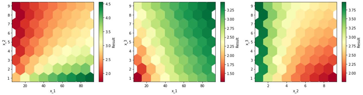
Figure 4.9 – Plot of sensitivity analysis

Three graphs have been drawn; this is because there are three input variables. To be able to appreciate the variability of the output as a function of the variability of the inputs, three graphs were drawn that couple the input variables into pairs.

By analyzing the third graph on the right, we can see, for example, that for low values of x_2, the x_3 variable seems irrelevant: when it changes, the output remains unchanged. We can appreciate this from the hexadecimal color map, which shows the same color for the entire range of variability of x_3. As the values of x_2 increase, there is a variability of the output, even as x_3 varies.

In the next section, we will learn how to evaluate the average information contained in data distributions. To do this, we will introduce the concepts of Cross-entropy.

Explaining the cross-entropy method

In Chapter 2, Understanding Randomness and Random Numbers, we introduced the entropy concepts in computing. Let’s recall these concepts.

First, there’s Shannon entropy. For a probability distribution, P={ p1, p2, ..., pN}, where pi is the probability of the N extractions, xi, of a random variable, X, Shannon defined the following measure, H, in probabilistic terms:

This equation has the same form as the expression of thermodynamic entropy and for this reason, it was defined as entropy upon its discovery. The equation establishes that H is a measure of the uncertainty of an experimental result or a measure of the information obtained from an experiment that reduces the uncertainty. It also specifies the expected value of the amount of information transmitted from a source with a probability distribution. Shannon’s entropy could be seen as the indecision of an observer trying to guess the result of an experiment or as the disorder of a system that can be under different configurations. This measure, defined as an information index, considers the only possibility that an event will happen or not, not its meaning or its value. This is the main limitation of the concept of entropy.

This equation would lead to maximum entropy if all probabilities were equal. The maximum entropy can be considered a measure of the total uncertainty. The statistically most probable state in which a system can find itself is that which corresponds to the maximum entropy. If there are two probability distributions with equally likely results, then it is possible to determine the differences in the information content of the two distributions.

The measure of entropy allows us to obtain a positive number. Since the probability is a number between 0 and 1, the logarithm of pi will take on a negative value, reaching the maximum value of 0 when the probability is equal to 1. For this reason, the minus sign before the sum allows us to obtain a value of positive entropy. From this, we can understand the use of Shannon’s entropy as a measure of uncertainty when distributing a random variable.

Introducing cross-entropy

Cross-entropy measures the accuracy of probabilistic forecasts, which is fundamental for modern forecasting systems since it allows us to produce very high-level estimates, even in the case of alternative indicators. Cross-entropy is very useful because it allows us to model even the rarest events, which are computationally expensive.

Cross-entropy measures the difference between two probability distributions for a given random variable or set of events. The information associated with an event quantifies the number of bits needed to encode and transmit it. Lower probability events provide more information; higher probability events provide less information. Cross-entropy tells us how likely an event is to happen based on its probability: if it is very probable, we have a small cross-entropy, while if it is not probable, we have a high cross-entropy.

At this point, we can define the cross-entropy: given two probability distributions, p and q, we can define the cross-entropy, H (p, q), with the following equation:

Here, x is the total number of values, p (x) is the probability of the real distribution (actual values), and q (x) is the probability of the distribution that was calculated, starting from the statistical model (predicted values).

If the expected values are equal to the current ones, then the cross-entropy and entropy are equal. In reality, this does not happen and the cross-entropy is obtained from the sum of the entropy and a term that takes the divergence into account.

Cross-entropy is commonly used in optimization procedures as a loss function. A loss function allows us to evaluate the performance of a simulation model: the better the model can predict the behavior of the real system, the smaller the values returned by the loss function. If we correct the algorithm to improve its predictions, then the loss function will give us a measure of the direction in which we are heading: if the loss function increasesm we are heading in the wrong direction, while if it decreases, we are heading in the right direction.

An algorithm based on cross-entropy provides for an iterative procedure in which each iteration can be divided into two phases:

1. A sample of random data is generated according to a specific mechanism.
2. We update the parameters of the random mechanism based on the data to produce a better sample in the next iteration.

Now, let’s learn how to calculate cross-entropy in a Python environment.

Cross-entropy in Python

Let’s start practicing with cross-entropy by applying the equation defined in the Introducing cross-entropy section to two artificially created distributions. Here is the Python code (cross_entropy.py):

from matplotlib import pyplot
from math import log2
events = ['A', 'B', 'C','D']
p = [0.70, 0.05,0.10,0.15] 
q = [0.45, 0.10, 0.20,0.25]
print(f'P = {sum(p):.3f}',f'Q = {sum(q):.3f}')
pyplot.subplot(2,1,1)
pyplot.bar(events, p)
pyplot.subplot(2,1,2)
pyplot.bar(events, q)
pyplot.show()
def cross_entropy(p, q):
    return -sum([p*log2(q) for p,q in zip(p,q)])
h_pq = cross_entropy(p, q)
print(f'H(P, Q) =  {h_pq:.3f} bits')

As always, we will analyze the code line by line:

1. Let’s start by importing the libraries:

   from matplotlib import pyplot

   from math import log2

The matplotlib library is a Python library for printing high-quality graphics. Next, we imported the log2() function from the math library. This library provides access to the mathematical functions defined by the C standard.

2. Now, let’s define the probability distributions:

   events = ['A', 'B', 'C','D']

   p = [0.70, 0.05,0.10,0.15] 

   q = [0.45, 0.10, 0.20,0.25]

   print(f'P = {sum(p):.3f}',f'Q = {sum(q):.3f}')

To start, we have defined four event labels so that we can identify them when plotted. Therefore, we have defined two lists with the probabilities associated with these events: recall that according to the definition of cross-entropy, with p, we indicate the probability of real distribution (actual values), while with q, we define the probability of the distribution that was calculated, starting from the statistical model (predicted values). Finally, after defining the two probability distributions, we made the sum to verify that it was equal to 1.

The following result is printed on the screen:

P = 1.000 Q = 1.000

3. Now, let’s draw the diagrams of the two distributions:

   pyplot.subplot(2,1,1)

   pyplot.bar(events, p)

   pyplot.subplot(2,1,2)

   pyplot.bar(events, q)

   pyplot.show()

We have plotted two bar graphs for the two probability distributions. A bar chart represents a series of data from different categories: it displays data using multiple bars of the same width, each representing a category. The height of each bar is proportional to the probability value. The following diagram is returned:

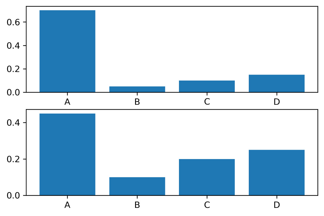
Figure 4.10 – Bar plot of probability distributions

4. Let’s define a function that calculates the cross-entropy by applying the equation we defined in the Introducing cross-entropy section:

   def cross_entropy(p, q):

       return -sum([p*log2(q) for p,q in zip(p,q)])

To do this, we used the zip () function, which returns a zip object. This is a tuple iterator. The two arguments we passed are coupled, element by element.

5. Now, let’s look at a new application in which we will use cross-entropy as a loss function. We can apply the function we just defined to the two previously defined probability distributions:

   h_pq = cross_entropy(p, q)

   print(f'H(P, Q) =  {h_pq:.3f} bits')

The following result is printed on the screen:

H(P, Q) =  1.505 bits

This represents the crossed entropy in bits. To verify its value, we can perform a new calculation simply by reversing the order of the distributions.

Binary cross-entropy as a loss function

Now, let’s look at a new application in which we will use cross-entropy as a loss function. We will do this for a binary classification case where the outputs belong to only two classes, (0,1). In this case, the loss is equal to the mean of the categorical cross-entropy loss on many two-category tasks. Cross-entropy loss is used to measure the performance of a classification model. The loss is calculated between 0 and 1, where 0 is a perfect model. The goal is generally to get the model as close to 0 as possible. The formula for calculating the cross-entropy changes slightly:

Here, N is the number of observations, y is the label (that is, the actual value), and p is the estimated probability.

In binary classification, the probability is modeled as the Bernoulli distribution for the class 1 label: the probability for class 1 is predicted directly by the model, and the probability for class 0 is given as 1 minus the predicted probability.

Here is the Python code (cross_entropy_loss_function.py):

import numpy as np
 
y = np.array([1.0, 0.0, 1.0, 0.0, 1.0, 0.0, 1.0, 0.0, 1.0, 0.0])
p = np.array([0.8, 0.1, 0.9, 0.2, 0.8, 0.1, 0.7, 0.3, 0.6, 0.4])
ce_loss = -sum(y*np.log(p)+(1-y)*np.log(1-p))
ce_loss = ce_loss/len(p) 
print(f'Cross-entropy Loss =  {ce_loss:.3f} nats')

As always, we will analyze the code line by line:

1. Let’s start by importing the libraries:

   import numpy as np

Here, we imported the numpy library, which offers additional scientific functions of the Python language, designed to perform operations on vectors and dimensional matrices.

2. Now, let’s define the probability distributions:

   y = np.array([1.0, 0.0, 1.0, 0.0, 1.0, 0.0, 1.0, 0.0, 1.0, 0.0])

   p = np.array([0.8, 0.1, 0.9, 0.2, 0.8, 0.1, 0.7, 0.3, 0.6, 0.4])

As mentioned previously, y is the label (that is, the actual value) and p is the estimated probability.

3. Let’s calculate the cross-entropy by applying the equation we defined previously:

   ce_loss = -sum(y*np.log(p)+(1-y)*np.log(1-p))

   ce_loss = ce_loss/len(p)
4. We just have to print the result:

   print(f'Cross-entropy Loss =  {ce_loss:.3f} nats')

The following result is returned:

Cross-entropy Loss = 0.272 nats

Note that the result is in nats and not in bits since we used the natural logarithm. nat is a logarithmic unit of information or entropy based on natural logarithms, rather than the base 2 logarithms that define the bit.

Summary

In this chapter, we addressed the basic concepts of Monte Carlo simulation. We explored the Monte Carlo components used to obtain a simulation with satisfactory results. Hence, we used Monte Carlo methods to estimate the value of Pi.

Then, we tackled two fundamental concepts of Monte Carlo simulation: the law of large numbers and the central limit theorem. For example, the law of large numbers allows us to determine the centers and weights of a Monte Carlo analysis to estimate definite integrals. The central limit theorem is of great importance, and it is thanks to this that many statistical procedures work.

Next, we analyzed practical applications of using Monte Carlo methods in real life: numerical optimization and project management. Finally, we learned how to perform numerical integration using Monte Carlo techniques.

Finally, sensitivity analysis concepts and cross-entropy methods were explained using some practical examples.

In the next chapter, we will learn the basic concepts of the Markov process. We will understand the agent-environment interaction process and how to use Bellman equations as consistency conditions for the optimal value functions to determine the optimal policy. Finally, we will learn how to implement Markov chains to simulate random walks.