
12
Simulating Models for Fault Diagnosis in Dynamic Systems
A physical system, in its life cycle, can be subject to failures or malfunctions that can compromise its normal operation. It is therefore necessary to introduce a fault diagnosis system within a plant capable of preventing critical interruptions. This is called a fault diagnosis system and it is capable of identifying the possible presence of a malfunction within the monitored system. The search for the fault is one of the most important and qualifying maintenance intervention phases and it is necessary to act in a systematic and deterministic way. To carry out a complete search for the fault, it is necessary to analyze all the possible causes that may have determined it.
In this chapter, we will learn how to approach fault diagnosis using a simulation model. We will start by exploring the basic concepts of fault diagnosis. Then, we will learn how to implement a model for fault diagnosis for a motor gearbox. In the last part of the chapter, we will analyze how to implement a fault diagnosis system for unmanned aerial vehicles.
In this chapter, we’re going to cover the following topics:
- Introducing fault diagnosis
- A fault diagnosis model for a motor gearbox
- A fault diagnosis system for an unmanned aerial vehicle
Technical requirements
In this chapter, we will learn how to use ANNs to simulate complex environments. To understand the topics, a basic knowledge of algebra and mathematical modeling is needed.
To work with the Python code in this chapter, you need the following files (available on GitHub at https://github.com/PacktPublishing/Hands-On-Simulation-Modeling-with-Python-Second-Edition):
- gearbox_fault_diagnosis.py
- UAV_detector.py
Introducing fault diagnosis
Diagnostics is a procedure for translating information, deriven from the measurement of parameters and from the collection of data relating to a machine and turned into information on actual or incipient failures of the machine itself. Diagnostics summarizes the complexity of analysis and synthesis activities, which, using the measurements of certain physical quantities and characteristics of the monitored machine, allow us to obtain significant information on the conditions of the machine itself and on its trend over time, for evaluations and forecasts on its short- and long-term reliability.
The use of fault diagnosis techniques is becoming increasingly important to ensure high levels of safety and reliability in automated and autonomous systems. In fact, in recent years, the international scientific community has produced considerable efforts to develop systematic approaches to the diagnosis of failures in systems of various kinds. The main purpose of a fault diagnosis scheme is to monitor a system during its operation to detect the occurrence of faults (fault detection), locate faults (fault isolation), and determine their temporal evolution (fault identification).
Understanding fault diagnosis methods
Typically, the output of a fault diagnosis system returns a set of sensitive variables from the type of faults, modified by an anomaly when the system is subject to failure. Then, the information contained in the occurrences of faults is extracted and processed to detect, isolate, and identify faults. The methods used for fault diagnostics can be grouped into three basic groups: model-based, knowledge-based, and data-based, as seen in Figure 12.1.

Figure 12.1: The group of methods used for fault diagnostics
Exploring the model-based approach
The model-based approach makes use of accurate mathematical models that allow both the detection and diagnosis of faults to be carried out efficiently. These models are based on the description of the actual degradation process of the components of interest. This specifically means modeling, in terms of the laws of physics, how the operating conditions affect the efficiency and longevity of assets. The most relevant variables include various thermal, mechanical, chemical, and electrical quantities. Being able to represent how they impact the health of machinery is a very complicated task. Therefore, the person who deals with creating this type of solution requires a high knowledge of the domain and modeling skills.
Important note
Once the model has been created, it is necessary to have sensors available that allows you to obtain values corresponding to the quantities considered relevant in the analysis and modeling phase to use them as inputs.
The main advantage of this type of approach is that it is descriptive; that is, it allows you to analyze the motivations of each output it provides, precisely because it is based on a physical description of the process. Consequently, it allows validation and certification. As for accuracy, it is strongly linked to the quality of analysis and modeling by domain experts. On the other hand, the negative aspects are the complexity and the high cost of implementation, together with the high specificity of the system, which entails little possibility of reuse and extension.
Describing the knowledge-based approach
The knowledge-based approach also relies on domain experts, as what you want to model with this type of approach is the skills and behavior of the experts themselves. The goal is to obtain a formalization of the knowledge they possess, to allow it to be reproduced and applied automatically.
Important note
Expert systems are in fact programs that use knowledge bases collected from people competent in each field and then apply inference and reasoning mechanisms on them to emulate thought and provide support and solutions to practical problems.
Among the most common approaches for implementing this type of model are rule-based mechanisms and fuzzy logic. The former has merits such as the simplicity of implementation and interpretability, but may not be sufficient to express complicated conditions and may suffer from a combinatorial explosion when the number of rules is very high. The use of fuzzy logic allows you to describe the state of the system through more vague and inaccurate inputs, making the process of formalization and description of the model simpler and more intuitive. Even for expert systems, as for model-based methods, the results are highly dependent on the quality and level of detail achieved by the model and are highly specific.
Discovering the data-based approach
The data-based approach applies statistical and machine learning techniques to the data collected by the machines, with the aim of then being able to recognize the status of the components.
Important note
The idea is to be able to obtain the greatest amount of information about the status of the machinery in real time, typically through sensors and from the logs of production and maintenance activities, and to correlate them with the level of degradation of the individual components or with the performance of the system.
This type of approach is currently the most used in practical cases. This is due to a series of advantages that this approach guarantees over the other two methods; data-driven approaches require large amounts of data to be effective, but with the availability of modern interconnected sensors (IIoT) this need is not difficult to satisfy. Compared to the other approaches, data driven approaches have the great advantage of not requiring in-depth knowledge specific to the application domain, thus making the contribution of the experts on the final performance of the model less decisive. The contribution of the experts can however be useful to speed up the selection process of the quantities to be used as input, but it has much less weight when compared with the other methods.
In addition, machine learning and data mining techniques may be able to detect relationships between the input parameters and the state of the system that even the experts themselves do not know a priori. Machine-learning-based algorithms can be used to develop predictive scenarios that allow us to extract knowledge about the specific domain
The machine-learning-based approach
Machine-learning-based algorithms automatically extract knowledge from data thanks to the data inputs received, without the need for specific commands from the developer. In these models, the machine can autonomously establish the patterns to be followed to obtain the desired result, this prerogative is typical of artificial intelligence. In the learning process that distinguishes these algorithms, the system receives a set of data necessary for training, estimating the relationships between the input and output data. These relationships represent the parameters of the model estimated by the system.
Problem definition
The choice of a specific model based on machine learning is highly dependent on the goal you want to achieve from the system. In fact, based on the objective, the problem is modeled differently. We can identify two approaches to the problem: diagnostics and prognostics. The purpose of a diagnostic system is to detect and identify a fault when the latter occurs. This, therefore, means monitoring a system, reporting when something is not working as expected, indicating which component is affected by the anomaly, and specifying the type of anomaly.
Prognostics, on the other hand, aim to determine whether a fault is close to occurring or to deduce the probability of occurrence. Obviously, prognostics being an a priori analysis, it can provide a greater contribution in terms of reducing the costs of interventions, but it is a more complex goal to achieve. Another option is to simultaneously use diagnostic and prognostic solutions applied to the same system. In fact, their combination provides two valuable advantages: diagnostics makes it possible to intervene to support decisions in cases where prognostics fail.
This scenario is in fact inevitable, as there are failures that do not follow a pattern that can be predicted, and even failures that are predictable with good precision cannot be identified in all their occurrences. The information obtained through diagnostic applications can be used as an additional input to predictive systems, thus allowing the creation of more sophisticated and precise models.
Binary classification
The simplest way is to represent the fault-finding as a binary classification problem, that is, in which every single input representing the state of the system must be labeled with one of two possible mutually exclusive values. In the event of a diagnostic problem, this means deciding whether the machine is functioning correctly or not correctly, making all possible states fall into these two classes. This is supervised learning, in the sense that the input data is provided with a label that represents the output of the model. In these cases, the system learns to recognize the relationships that bind the input data to the labels.
For prognostics, the interpretation becomes that of deciding whether the machine can fail within a set time interval. The difference between the two meanings is simply due to the different interpretations of the labels. This means that the same model can solve both problems. What will be differentiated is the labeling of the dataset used to carry out the model training phase.
Multiclass classification
The multiclass version is a generalization of binary classification, in which the number of possible labels to choose from is increased. However, only one label must be associated with each input.
The diagnostic case extends the previous case in a very intuitive way, that is, deciding whether the machine is functioning correctly or not correctly, and in the second case, which of the possible anomaly states. While the applications of prognostics you can see the problem is deciding in which time interval before the failure the machine is located, where then the possible labels represent different intervals of proximity to a failure.
Regression
Regression can be used to model prognostic problems. This means that the remaining useful life of a component can be estimated in terms of a continuous number of predetermined time units. In this specific case, the training dataset must only contain data relating to components that have been subject to failures, to allow the labeling of the inputs backward starting from the instant of failure.
This approach to the problem also provides a supervised learning paradigm, in this case, the input data will be associated with continuous output values.
Anomaly detection
A further possible representation for diagnostic problems is to consider it as an anomaly detection problem. This means that the model must be able to establish whether the operation of the machine returns to a normal state or if it deviates from it, that is, re-entering a case of anomaly.
The interpretation of the problem is, therefore, very similar to that of the binary classification. However, this methodology differs from the classification since it falls within the cases of semi-supervised learning, as the model only needs to learn from inputs that represent correct operating states and must, following the training phase, recognize unknown anomalous states, that is, of which the model does not know the characteristics.
Data collection
For an accurate diagnosis of faults in complex machines, it is essential to acquire information through the collection of data, analyze this data using advanced signal processing algorithms and, finally, extract the appropriate functionalities for efficient identification and classification of faults.
The data can be collected through different methodologies—through the measurements of all those physical quantities that somehow describe the state of the machine during its operation. They are obtained through special sensors that convert the physical value into an electrical value called sensor data.
Important note
Examples of these parameters used are noise, vibrations, pressure, temperature, and humidity, whereby the relevance of each of them strongly depends on the system being monitored.
Typically, an industrial system based on modern automation already has all the data necessary for its diagnostics available. If they are not available, the addition of additional sensors is the first step to implementing a correct fault identification strategy. But the data can also be collected by correlating the static operating conditions of the machine or plant to each instant of time, such as the code of the materials used, the production speed of the machine, and the type of piece produced. In this case, statistical data is defined.
Finally, the data can collect the history of relevant events and actions concerning a machine and its components. This data is called log data and may contain, for example, the history of faults found or repairs and replacements.
After having explored the basic concepts of fault diagnosis, it is now time to practically tackle a simulation problem.
Fault diagnosis model for a motor gearbox
The combustion engine delivers power within a narrow rev range. The tractive force is transmitted to the wheels under varying load situations through gear pairs. The more ratios there are, the better the engine work can be adapted to parameters such as acceleration, slope, load, consumption, and noise. To maintain engine operation within its optimal range of use, it is essential to be able to vary the transmission ratio between the engine itself and the drive wheels. In order to satisfy this need, it is necessary to insert a device generally defined as a mechanical gearbox between the motor and the wheels, which allows the motor to be used in an operating range capable of satisfying the needs of the users.
By using a fixed transmission ratio between the engine and the wheels, a curve is obtained that allows the maximum power of the engine to be exploited at a single-speed value. However, even if you have a stepped gearbox with a finite number of ratios, you can only get close to optimal exploitation of the engine since an infinite number of operating conditions cannot in any case be reached.
The gearbox consists of the following mechanical components: input drive shaft, countershaft, and output drive shaft. On these three components are sprockets of different sizes, meshed with each other, which correspond to the different gears, or torque ratios. Through the use of the clutch and the gear lever, it is possible to freely decide which gear to use according to need; in general, a higher gear corresponds to a higher speed.
Since these are mechanical components subjected to contact with each other, the components of a gearbox are subject to wear, which can also lead to breakage. In the case of breakage, the engine obviously stops and requires the replacement of the gearbox components. An automatic fault identification system can ensure that a problem is detected before the gearbox fails.
In this example, we will use data detected by accelerometers that measured the vibrations of a gearbox in correspondence with two operating conditions: healthy, and broken. The sensors were placed in opposite directions in order to detect all possible changes in operation. These data will be used to train different algorithms for the classification of the operating conditions of the gearbox.
The dataset is available on the Kaggle open data repository, which offers numerous projects to use to train machine learning-based algorithms. In its original version, the dataset is available at the following URL:
https://www.kaggle.com/datasets/brjapon/gearbox-fault-diagnosis
In this section, we have reduced the dataset’s size to avoid the unnecessary burden of the calculations. The dataset offers the measurements of the vibrations detected by two sensors and the corresponding classification of the engine operation: 0 = broken, 1 = healthy.
As always, we will analyze the code line by line:
- We will start by importing the libraries:
import pandas as pd
import seaborn as sns
from matplotlib import pyplot as plt
from sklearn.model_selection import train_test_split
from sklearn.linear_model import LogisticRegression
from sklearn.ensemble import RandomForestClassifier
from sklearn.neural_network import MLPClassifier
from sklearn.neighbors import KNeighborsClassifier
from sklearn.inspection import DecisionBoundaryDisplay
The pandas library is an open source BSD-licensed library that contains data structures and operations to manipulate high-performance numeric values for the Python programming language. The seaborn library is a Python library that enhances the data visualization tools of the matplotlib module. In the seaborn module, there are several features we can use to graphically represent our data. There are methods that facilitate the construction of statistical graphs with matplotlib. The matplotlib library is a Python library for printing high-quality graphics. Then, we imported a series of models that we will analyze in detail and discuss where we will use them.
- Now, we can upload the data:
data = pd.read_excel(‘fault.dataset.xlsx’)
To do this, we’ll use the read_excel module of the pandas library. The read_excel method reads an Excel table into a pandas DataFrame.
- Before starting with data analysis, we will conduct an exploratory analysis to understand how the data is distributed and extract preliminary knowledge. To display the first 10 rows of the DataFrame imported, we can use the head() function, as follows:
print(data.head(10))
The first 10 rows are displayed, as follows:
          a1        a2  state
0   2.350390  1.454870      0
1   2.452970  1.400100      0
2  -0.241284 -0.267390      0
3   1.130270 -0.890918      0
4  -1.296140  0.980479      0
5  -1.650290  1.011530      0
6   0.429159 -1.163700      0
7  -0.191893 -2.945480      0
8   1.417660 -3.317650      0
9   1.699620 -2.446150      0
As we can see, there are three columns of data in the dataset: the measurements of the vibrations detected by two sensors (a1, and a2) and the corresponding classification of the engine operation.
- To extract some information, we can invoke the info() function, as follows:
print(data.info())
This method prints a concise summary of a DataFrame, including the dtype index, dtypes column, non-null values, and memory usage. The following results are returned:
<class ‘pandas.core.frame.DataFrame’>
RangeIndex: 20000 entries, 0 to 19999
Data columns (total 3 columns):
 #   Column  Non-Null Count  Dtype
---  ------  --------------  -----
 0   a1      20000 non-null  float64
 1   a2      20000 non-null  float64
 2   state   20000 non-null  int64
dtypes: float64(2), int64(1)
memory usage: 468.9 KB
None
Useful information is reported—the numbers of the entries (20,000) and data columns (3). Essentially, the list of all features with the number of elements, the possible presence of missing data, and the type is returned. In this way, we can already get an idea of the type of variables we’re about to analyze. In fact, analyzing the results obtained, we note that two types have been identified: float64 (2) and int64 (1).
- To get a preview of the data contained in it, we can calculate a series of basic statistics. To do so, we’ll use the describe() function in the following way:
DataStat = data.describe()
print(DataStat)
The following results are returned:
                 a1            a2         state
count  20000.000000  20000.000000  20000.000000
mean       0.024046      0.006011      0.500000
std        5.897926      4.231061      0.500013
min      -36.989500    -23.710700      0.000000
25%       -3.107135     -2.360157      0.000000
50%       -0.043941      0.071639      0.500000
75%        3.011813      2.520958      1.000000
max       33.375500     20.906000      1.000000
The describe() function generates descriptive statistics that summarize the central tendency, dispersion, and shape of a dataset’s distribution, excluding NaN values. It analyzes both numeric and object series, as well as DataFrame column sets of mixed data types.
- So far we have not had evidence that the third variable (state) represents a dichotomous variable. To do this, we can use the describe function but pass the arguments as data of the type object:
DataStatCat = data.astype(‘object’).describe()
print(DataStatCat)
The following results are returned:
                 a1           a2  state
count   20000.00000  20000.00000  20000
unique  19888.00000  19877.00000      2
top        -1.93396      1.32888      0
freq        2.00000      2.00000  10000
As we can see, the state variable has only two values, and each value has an occurrence of 1,000.
- To continue in our preventive visual analysis of the data, let us now use the graphs to help us. For example, we can draw boxplots of the distribution of the data detected by the two sensors (a1, a2):
fig, axes = plt.subplots(1,2, figsize=(18, 10))
sns.boxplot(ax=axes[0],x=’state’, y=’a1’, data=data)
sns.boxplot(ax=axes[1],x=’state’, y=’a2’, data=data)
plt.ylim(-40, 40)
plt.show()
A boxplot is a graphical representation used to describe the distribution of a sample by simple dispersion and position indexes. To draw a boxplot of a DataFrame, we used the seaborn package. The following chart is returned:
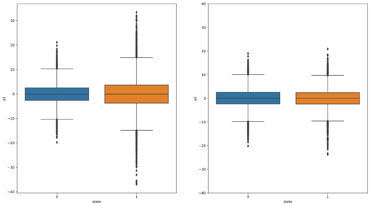
Figure 12.2: A boxplot of sensor measurement data
Through analyzing Figure 12.2, we can see that the distributions of the data collected by the two sensors are different. Sensor a1 seems to diversify the vibration values between broken and healthy conditions. This suggests that faults are occurring at the location of this sensor.
- At this point, it is necessary to divide the data into input (X) and target (Y), this is necessary to train our algorithm for the classification of the operating conditions:
X = data.drop(‘state’, axis = 1)
print(‘X shape = ',X.shape)
Y = data[‘state’]
print(‘Y shape = ',Y.shape)
- After separating the target from the input data, it is necessary to divide the data into two groups, the first group will be used to train the classification algorithms, and the second to evaluate its performance.
To do this, we will use the train_test_split() function:
X_train, X_test, Y_train, Y_test = train_test_split(X, Y, test_size = 0.30, random_state = 1)
print(‘X train shape = ',X_train.shape)
print(‘X test shape = ', X_test.shape)
print(‘Y train shape = ', Y_train.shape)
print(‘Y test shape = ',Y_test.shape)
The train_test_split() function splits arrays or matrices into random train and test subsets. Four arguments are passed: The first two arguments are X (Input) and Y (target) pandas Dataframe. The last two arguments are as follows:
- test_size: This should be between 0.0 and 1.0, and represents the proportion of the dataset to include in the test split
- random_state: This is the seed used by the random number generator
- Finally, we print the dimensions of the four datasets we obtained on the screen:
X train shape = (14000, 2)
X test shape = (6000, 2)
Y train shape = (14000,)
Y test shape = (6000,)
- After carefully splitting the data, we can train our algorithms. Let’s start with a model based on logistic regression:
lr_model = LogisticRegression(random_state=0).fit(X_train, Y_train)
lr_model_score = lr_model.score(X_test, Y_test)
print(‘Logistic Regression Model Score = ', lr_model_score)
In a logistic regression model, the response variable is a binary or dichotomous variable. Variables of this type are configured as variables that can only assume two mutually exclusive values, in this case, 0 or 1. By exploiting statistical methods, it is possible, through the use of logistic regression, to calculate the probability that an observation or input belongs to a class or not. Logistic regression is in fact a predictive analysis that is used to evaluate the relationship between a dependent variable and one or more independent variables, estimating probabilities through a logistic function. The probabilities then turn into binary values in order to make a prediction.
To train a logistic-regression-based model we used the LogisticRegression () function of the sklearn.linear_model module. The sklearn.linear_model module contains several functions to resolve some problems, such as regression problems and classification problems. The LogisticRegression () function implements regularized logistic regression using the liblinear library and the newton-cg, sag, saga, and lbfgs solvers. After having trained the model, we tested it with the use of data so far never seen by the algorithm (X_test, Y_test). The following results were obtained:
Logistic Regression Model Score = 0.49333333333333335
This tells us that only half of the data has been correctly classified. This is a confidence score, a number between 0 and 1 that represents the probability that the forecast model output is correct.
- So, let’s see the results of the classification in visual form. To do this, we will trace a graph showing the two data classes and then trace the contours of the classification domain:
ax1 = DecisionBoundaryDisplay.from_estimator(
lr_model, X_train, response_method=”predict”,
alpha=0.5)
ax1.ax_.scatter(X_train.iloc[:,0], X_train.iloc[:,1], c=Y_train, edgecolor=”k”)
plt.show()
To trace the contours of the classification domain, we used the DecisionBoundaryDisplay () function of the sklearn.inspection model. The sklearn.inspection module helps us identify what influences a model’s predictions to better understand them. We can leverage the tools offered by this module to evaluate model assumptions and biases, design a better model, or diagnose problems with model performance. The following diagram is printed:
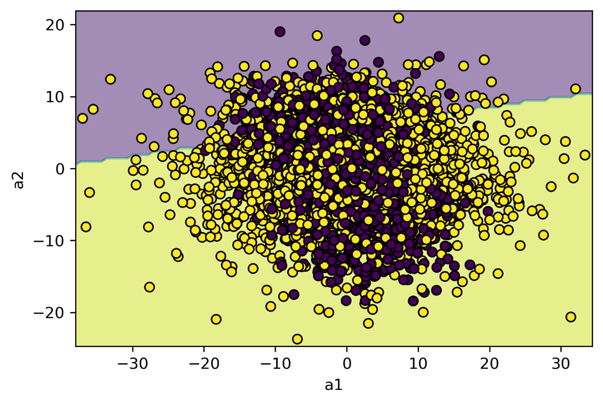
Figure 12.3: The distribution of the two classes of functioning with the decision boundaries returned by the model based on the logistic regression
Figure 12.3 clearly shows that the two classes overlap in the space of the two features (a1, a2). The space is therefore divided by the model into two parts, but this division cannot effectively identify the two classes (score = 0.49).
- So, let’s see if we can improve the performance of the classifier using the random forest algorithm:
rm_model_score = rm_model.score(X_test, Y_test)
print(‘Random Forest Model Score = ', rm_model_score)
When you want to get the prediction of a certain event, it is more effective to use a set of predictors rather than the best single predictor, almost always obtaining better predictions. The group of predictors is called an ensemble and this technique is called ensemble learning. An algorithm that takes advantage of this methodology is called the ensemble method. A group of decision trees, each with a different random subset of the training set, that provides a final prediction is called the random forest and is one of the most powerful machine learning algorithms, despite its simplicity. The random forest algorithm is, therefore, a set of decision trees generally trained with the bagging method and can be used for discrete problems, classification, or continuous regression, the latter constituting the present case. This algorithm adds further randomness, in addition to the assignment of subsets of the training set to individual predictors: instead of searching for the best feature as a condition for splitting a node, it finds the best feature in a random subset of the global set of features themselves. This leads to a greater diversity of individual decision trees.
To train a random-forest-based model, we used the RandomForestClassifier() function from the sklearn.ensemble module. The following two arguments were passed:
- max_depth: The maximum depth of the tree
- random_state: The randomness of the bootstrapping of the samples used
In addition to these, the two input variables and the target are passed. Once again, we tested it with the use of data so far never seen by the algorithm (X_test, Y_test). The following results were obtained:
Random Forest Model Score = 0.5838333333333333
We have significantly improved the performance of the classifier, but we are still far from a satisfactory result. Let’s now see the visual classification:
ax2 = DecisionBoundaryDisplay.from_estimator(
    rm_model, X_train, response_method=”predict”,
     alpha=0.5)
ax2.ax_.scatter(X_train.iloc[:,0], X_train.iloc[:,1], c=Y_train, edgecolor=”k”)
plt.show()
The following diagram is returned:

Figure 12.4: The distribution of the two classes that are functioning with the decision boundaries returned by the model based on the random forest classifier
In this case, we can see that the domain has been divided more selectively to demonstrate the performance improvement returned by the classifier.
- But we are not satisfied; let’s see what we get by applying the ANNs that have always behaved well in the classification:
mlp_model = MLPClassifier(random_state=1, max_iter=300).fit(X_train, Y_train)
mlp_model_score = mlp_model.score(X_test, Y_test)
print(‘Artificial Neural Network Model Score = ', mlp_model_score)
In Chapter 10, Simulating Physical Phenomena Using Neural Networks, we explored the extreme versatility of neural networks in dealing with both regression problems and classification problems. In this example, we used the MLPClassifier() function from the sklearn.neural_network module. This module includes models based on neural networks. The MLPClassifier() function implements a multi-layer perceptron classifier; two arguments are passed:
- random_state: Random number generation for weights and bias initialization
- max_iter: Maximum number of iterations
In addition to these, the two input variables and the target are passed. Once again, we tested it with the use of data so far never seen by the algorithm (X_test, Y_test). The following results were obtained:
Artificial Neural Network Model Score = 0.5955
We got a further improvement in the classification; let’s see it in a graph:
ax3 = DecisionBoundaryDisplay.from_estimator(
    mlp_model, X_train, response_method=”predict”,
     alpha=0.5)
ax3.ax_.scatter(X_train.iloc[:,0], X_train.iloc[:,1], c=Y_train, edgecolor=”k”)
plt.show()
The following diagram is printed:
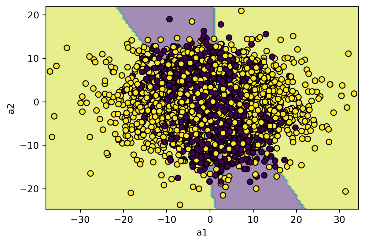
Figure 12.5: Distribution of the two classes that are functioning with the decision boundaries returned by the model based on the ANN classifier
In Figure 12.5, we can see a further improvement in the subdivision of the domain confirming the improvement in the performance of the classifier.
- Finally, let’s try to see what happens by delving into a classifier based on the K-nearest neighbors algorithm:
kn_model_score = kn_model.score(X_test, Y_test)
print(‘K-nearest neighbors Model score =', kn_model_score)
K-nearest neighbors (KNN) is a supervised machine learning algorithm for classification. It is called a lazy learner, as it does not learn a rule on how to discriminate vector classes, but stores the entire learning dataset. The algorithm itself is quite simple and can be summarized in the following steps:
- Choose the number k and a metric for the distance
- Find the k elements closest to the sample to be classified
- Assign the class label with a majority vote
Based on the chosen metric, the KNN algorithm finds the k samples in the learning dataset that are closest (most similar) to the point to be classified. The class of the new point is then determined by a majority vote based on the class to which its k neighbors belong. The main advantage of this memory-based approach is that the classifier adapts immediately as we add learning vectors. On the other hand, the flaw is that the computational complexity for classifying new samples grows at most linearly with the number of learning vectors. Moreover, we cannot a priori ignore any training vector since there is no real learning. Thus, storage space and the number of distances to be calculated can become a nodal problem when working with large datasets.
We used the K-neighborsClassifier() function from the sklearn.neighbors module. This module contains useful tools for training unsupervised and supervised neighbor-based learning algorithms. Only one argument was passed:
- n_neighbors: The number of neighbors to use
The following score was returned:
K-nearest neighbors Model score = 0.5531666666666667
In this case, we have not obtained an improvement compared to the last two algorithms applied, but in any case, the result is better than the results obtained with the logistic regression.
Let’s see what happens in the classification domain:
ax4 = DecisionBoundaryDisplay.from_estimator(
    kn_model, X_train, response_method=”predict”,
     alpha=0.5)
ax4.ax_.scatter(X_train.iloc[:,0], X_train.iloc[:,1], c=Y_train, edgecolor=”k”)
plt.show()
The following diagram is printed:
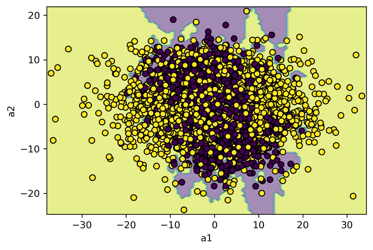
Figure 12.6: The distribution of the two classes that are functioning with the decision boundaries returned by the model based on the KNN algorithm
The boundary decisions seem more localized in correspondence between the two classes, but the difficulty in classifying the data is still evident.
After having seen how to elaborate simulation models of systems for automatic identification of engine gearbox failures, let’s now see what happens when we try to simulate a drone failure identification system.
Fault diagnosis system for an unmanned aerial vehicle
Technological development has led to the birth of aircraft with remarkable capabilities capable of autonomously managing flight. This category, known as unmanned aerial vehicles (UAVs), are vehicles that fly unmanned, which brings the advantages of a drastic reduction in operating costs compared to conventional aircraft with a pilot, the ability to operate in environments unsuitable for human presence, and to be used in a timely manner for overhead detection, for example, of natural disasters. Initially used exclusively in the military field – in dull missions (monotonous and long-lasting surveillance and reconnaissance), dirty missions (dangerous for the safety of pilots), and dangerous missions (risky for the lives of pilots) – today they represent the future of modern aeronautics. The enormous potential, the successes in military missions, and the progress made in the field of micro- and nano-technologies are pushing both industries and universities to develop ever more modern, reliable UAV systems capable of being used in a wide spectrum of civilian and military missions.
The wide diffusion of UAVs that is occurring in the world highlights new problems that have not yet been explored. The convenience of using these devices is accompanied by the problems and dangers associated with this technology. One of the problems that have been raised concerns the safety of the flight of such devices – what happens if a UAV crashes to the ground? Furthermore, given the small size of the UAVs, they are hard to identify with radar systems. This feature was immediately exploited by malicious people who used them for fraudulent purposes. The use of drones to transport drugs and smartphones into prisons, up to the use of drones for terrorist attacks, is the news of recent times. In these scenarios, the development of an automatic system for detecting the presence of UAVs in complex urban scenarios becomes crucial.
In this example, we will see how to identify the presence of a UAV based on monitoring the WiFi traffic detected in the vicinity of a sensitive target.
To do this, we will use a dataset available on the UCI Machine Learning Repository site at the following URL:
https://archive.ics.uci.edu/ml/datasets/Unmanned+Aerial+Vehicle+%28UAV%29+Intrusion+Detection
As always, we will analyze the code line by line:
- We will start by importing the libraries:
import pandas as pd
from sklearn.model_selection import train_test_split
from sklearn.svm import SVC
import matplotlib.pyplot as plt
from sklearn.feature_selection import SelectKBest, chi2
The pandas library is an open source BSD-licensed library that contains data structures and operations to manipulate high-performance numeric values for the Python programming language. Then, we imported the train_test_split() function from sklearn.model_selection module, and the SVC() function from sklearn.svm module. To trace the diagrams, we first imported the matplotlib library, and finally, we imported the SelectKBest() and chi2() functions from the sklearn.feature_selection module. A detailed description of these functions will be proposed and where they will be used.
- Let’s move on to importing the dataset:
data = pd.read_excel(‘UAV_WiFi.xlsx’)
To do this, we used the read_excel module of the pandas library. The read_ excel method reads an Excel table into a pandas DataFrame.
Before starting with data analysis, we will conduct an exploratory analysis to understand how the data is distributed and extract preliminary knowledge. To display some statistics, we will use the info() function as follows:
print(data.info())
The following data is returned:

Figure 12.7: Dataset features list with the number of occurrences and type of data
This list allows us to identify all the features present in the dataset. We can see that there are 17629 data records, 54 features of which 53 represent the input data and the last feature, named target, represents the data classification label (1 = UAV, 0 = No UAV).
Let’s extract other statistics from the data:
DataStatCat = data.astype(‘object’).describe()
print(DataStatCat)
The following data is listed:
         uplink_size_mean  ...  target
count        17629.000000  ...   17629
unique       17622.000000  ...       2
top              0.003465  ...       1
freq             2.000000  ...    9760
The most interesting thing concerns the target variable, wherein, we have the confirmation that it is binomial data (only two types of occurrences), and that the distribution of the two categories is sufficiently balanced (the frequency of class 1 is equal to 9760, this means that the other class is present with a frequency equal to 17629 - 9760 = 7869).
- Now, we can separate the input data from the target:
X = data.drop(‘target’, axis = 1)
print(‘X shape = ',X.shape)
Y = data[‘target’]
print(‘Y shape = ',Y.shape)
The following results are displayed:
X shape =  (17629, 54)
Y shape =  (17629,)
- To properly train the classifier that will allow us to identify the presence of the UAV near the sensitive target, it is necessary to divide the data into two sets. The first set will be used for training, while the other will be used to verify the correct operation of the classifier:
X_train, X_test, Y_train, Y_test = train_test_split(X, Y, test_size = 0.30, random_state = 1)
print(‘X train shape = ',X_train.shape)
print(‘X test shape = ', X_test.shape)
print(‘Y train shape = ', Y_train.shape)
print(‘Y test shape = ',Y_test.shape)
The train_test_split() function splits arrays or matrices into random train and test subsets. The following results are printed:
X train shape =  (12340, 54)
X test shape =  (5289, 54)
Y train shape =  (12340,)
Y test shape =  (5289,)
We will, therefore, use 70% of the data for training and the remaining 30% for testing.
- Now, let’s train a support-vector-based classifier:
SVC_model = SVC(gamma=’scale’,
random_state=0).fit(X_train, Y_train)
SVC_model_score = SVC_model.score(X_test, Y_test)
print(‘Support Vector Classification Model Score = ', SVC_model_score)
Support vector machines (SVM) are a set of supervised learning methods for regression and pattern classification, developed in the 1990s by Bell AT&T laboratories. They are known as maximum margin classifiers, as they minimize the classification error and maximize the distance margin. SVM can be thought of as an alternative technique for learning polynomial classifiers, as opposed to the classical training techniques of neural networks. Single-layer neural networks have an efficient learning algorithm but are only useful in the case of linearly separable data. Conversely, multilayer neural networks can represent nonlinear functions. But these are difficult to train due to a large number of dimensions of the weight space and because the most popular techniques, such as backpropagation, allow you to obtain the network weights by solving a problem non-convex and unconstrained optimization system, which, consequently, has an indeterminate number of local minima.
The SVM training technique solves both problems. It has an efficient algorithm and is capable of representing complex nonlinear functions. The characteristic parameters of the network are obtained by solving a convex quadratic programming problem with equality or box-type constraints (in which the value of the parameter must be kept within an interval), which provides for a single global minimum.
To train the SVM-based model, we used the SVC () function of the sklearn.svm module. The following two parameters were passed:
- gamma: Kernel coefficient: We used a scale kernel that fix gamma = 1 / (n_features * X.var())
- Random state: Controls the pseudo-random number generation for the reproducibility of the example
We then tested the model trained on the test data. The following results were obtained:
Support Vector Classification Model Score = 0.5517110985063339
This is the mean accuracy of the model. The accuracy of the classification model returns the percentage of correct predictions on a dataset used for testing that the model has never seen in the training process. This is equivalent to the ratio of the number of correct estimates to the total number of input samples.
Just over 50% of correct classifications do not satisfy us, so let’s see how to improve the performance of the classifier. When using the input features to classify a target the different variability of the features can affect the result.
To evaluate the different variability of the data of the input features, we can draw boxplots of the first five features:
first_10_columns = X.iloc[:,0:5]
plt.figure(figsize=(10,5))
first_10_columns.boxplot()
The following boxplot is displayed:

Figure 12.8: A boxplot of the first five features of the input data
We can see that the range of variability is very different already for these first five features; who knows what acacde for the others. In these cases, it is advisable to scale the data. As we saw in Chapter 10, Simulating Physical Phenomena Using Neural Networks, we can reduce the values so that they fall within a common range, guaranteeing the same characteristics of variability possessed by the initial dataset. In this way, we will be able to compare variables belonging to different distributions and variables expressed in different units of measurement.
In this example, we will use the min-max method (usually called feature scaling) to get all of the scaled data in the range [0 – 1]. The formula to achieve this is as follows:

We just have to rewrite this formula in Python:
X_scaled = (X-X.min())/(X.max()-X.min())
Now, let’s check how the data variability has changed by drawing a boxplot of the first five features of the input dataset:
first_10_columns = X_scaled.iloc[:,0:5]
plt.figure(figsize=(10,5))
first_10_columns.boxplot()
The following boxplot is displayed:
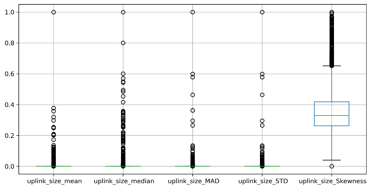
Figure 12.9: A boxplot of the first five features of the input data after the data scaling
After looking at Figure 12.9 and comparing it with Figure 12.8, we can see that now the range of variability of the data has been significantly reduced. Now, all the variables vary in the range [0 – 1].
- But this may not be enough to improve the performance of the classifier, so let’s make a feature selection. Feature selection is based on finding a subset of the original variables, usually iteratively, thus detecting new combinations of variables and comparing prediction errors. The combination of variables that produces the minimum error will be labeled as a selected feature and used as input for the machine learning algorithm. To perform the feature selection, we must set the appropriate criteria in advance. Usually, these selection criteria determine the minimization of a specific predictive error measure for models fit for different subsets. Based on these criteria, the selection algorithms seek a subset of predictors that optimally model the measured responses. Such research is subject to constraints, such as the necessary or excluded characteristics and the size of the subset.
To perform feature selection, we will apply the SelectKBest() function as follows:
best_input_columns = SelectKBest(chi2, k=10).fit(X_scaled, Y)
sel_index = best_input_columns.get_support()
best_X = X_scaled.loc[: , sel_index]
The SelectKBest() function selects features according to the k highest scores: this function adopts as a parameter a score function, which is applied to the pair (X_scaled, Y). The score function returns an array of scores. The function then selects only the features that record the highest scores. The chi2 () function was used as the scoring function, which computes chi-squared stats between each non-negative feature and class.
After selecting the best 10 features, we extracted them from the starting dataset and created a new input dataset with only the best 10 features (best_X).
Out of curiosity, let’s see what they are:
feature_selected = best_X.columns.values.tolist()
print(“The best 10 feature selected are:", feature_selected)
The following features are selected:
The best 10 feature selected are: [' downlink_size_mean’, ' downlink_size_median’, ' downlink_size_MAD’, ' downlink_size_MAX’, ' downlink_size_MIN’, ' downlink_size_MeanSquare’, ' uplink_interval_STD’, ' uplink_interval_Kurtosis’, ' uplink_interval_MIN’, ' both_links_interval_MIN’]
Now that we have a new dataset with the best features, let’s split the data again (70% for training, 30% for testing):
X_train, X_test, Y_train, Y_test = train_test_split(best_X, Y, test_size = 0.30, random_state = 1)
print(‘X train shape = ',X_train.shape)
print(‘X test shape = ', X_test.shape)
print(‘Y train shape = ', Y_train.shape)
print(‘Y test shape = ',Y_test.shape)
The following subsets are created:
X train shape =  (12340, 10)
X test shape =  (5289, 10)
Y train shape =  (12340,)
Y test shape =  (5289,)
Now, we can finally re-train the SVM-based classification model:
SVC_model = SVC(gamma=’auto’,random_state=0).fit(X_train, Y_train)
SVC_model_score = SVC_model.score(X_test, Y_test)
print(‘Support Vector Classification Model Score = ', SVC_model_score)
The following result is returned:
Support Vector Classification Model Score = 1.0
Not a bad improvement, we went from a support vector score of 0.55 to 1.0.
Summary
In this chapter, we learned how to approach fault diagnosis using simulation models. We started by exploring the basic concepts of fault diagnosis. Then, we learned how to implement a model for fault diagnosis for a motor gearbox. Finally, we analyzed how to implement a fault diagnosis system for unmanned aerial vehicles.
In the next chapter, we will summarize the simulation modeling processes we looked at in the previous chapters. Then, we will explore the main simulation modeling applications that are used in real life. Finally, we will discover future challenges regarding simulation modeling.