8

Introducing Evolutionary Systems

Evolutionary algorithms are a family of stochastic techniques for solving problems that are part of the broader category of natural metaphor models. They find their inspiration in biology and are based on the imitation of the mechanisms of so-called natural evolution. Over the last few years, these techniques have been applied to many problems of great practical importance.

In this chapter, we will learn the basic concepts of SC and how to implement genetic programming. We will also understand the genetic algorithm techniques, how to implement symbolic regression, and how to use the cellular automata (CA) model.

In this chapter, we’re going to cover the following main topics:

• Introducing SC
• Understanding genetic programming
• Applying a genetic algorithm for search and optimization
• Performing symbolic regression
• Exploring the CA model

Technical requirements

In this chapter, we will learn how to use genetic programming to optimize systems. To deal with the topics in this chapter, it is necessary that you have a basic knowledge of algebra and mathematical modeling. To work with the Python code in this chapter, you’ll need the following files (available on GitHub at the following URL: https://github.com/PacktPublishing/Hands-On-Simulation-Modeling-with-Python-Second-Edition):

• genetic_algorithm.py
• symbolic_regression.py
• cellular_automata.py

Introducing SC

Over the past few decades, many researchers have developed numerous methods and systems, many of which have been successfully used in real-world applications. In these applications, most of the methods are based on probabilistic paradigms, such as the well-known Bayesian inference, rules of thumb, and decision systems. Since the 1960s, several great and epoch-making theories have been proposed using fuzzy logic, genetic algorithms, evolutionary computation, and neural networks – all methods that are referred to as SC. When combined with well-established approaches to probability, these new SC methods become effective and powerful in real-world applications. The ability of these techniques to include inaccuracy and incompleteness of information and model very complex systems makes them useful tools in many sectors.

SC takes on the following characteristics:

• The ability to model and control uncertain and complex systems, as well as to represent knowledge efficiently through linguistic descriptions typical of fuzzy set theory
• The ability to optimize genetic algorithms whose computation is inspired by the laws of selection and mutation typical of living organisms
• The ability to learn complex functional relationships as in the case of neural networks, inspired by those in brain tissue

In the SC, among its characteristic features, we find, in fact, uncertain, ambiguous, or incomplete data, consistent parallelism, randomness, approximate solutions, and adaptive systems.

Important note

The constitutive methodologies of SC require considerable computing powers; all, in fact, presuppose a significant computational effort, which only modern computers have made it possible to sustain in a reasonable time.

From a historical point of view, we can consider that neural networks were born in 1959, fuzzy logic in 1965, probabilistic reasoning in 1967, and genetic algorithms in 1975. Originally, each algorithm had well-defined labels and usually could be identified with specific scientific communities. In recent years, by improving the understanding of the strengths and weaknesses of these algorithms, we have begun to make the most of their characteristics and the development of hybrid algorithms. These denominations indicate a new integration trend that reflects the current high degree of integration between scientific communities. These interactions have given birth to SC, a new field that combines the versatility of fuzzy logic to represent qualitative knowledge with efficient data from neural networks to provide adequate refinements through a local search, and the ability of genetic algorithms to efficiently perform a global search. The result is the development of hybrid algorithms that are superior to each underlying component of SC, providing us with the best real-world problem-solving tools.

At the beginning of this section, we said that under the name of SC, there are several theories: fuzzy logic, neural networks, evolutionary computation, and genetic algorithms. Let us now see a brief description of these methodologies.

Fuzzy logic (FL)

FL corresponds to a mathematical approach to translating the fuzziness of linguistic concepts into a representation that computers can understand and manipulate. Since FL can transform linguistic variables into numerical ones without losing the sense of truth along the way, it allows for the construction of improved models of human reasoning and in-depth knowledge. FL and fuzzy set theory in general provide an approximate indication, an effective and flexible tool, to describe the behavior of systems that are too complex or too ill-defined to admit a precise mathematical analysis with classical methods and tools. Since fuzzy set theory is a generalization of classical set theory, there is more flexibility to faithfully capture the various aspects of an information situation under conditions of incompleteness or ambiguity. In this way, in addition to operating only with linguistic variables, modern fuzzy set systems are designed to manage any type of information uncertainty.

Artificial neural network (ANN)

ANNs take inspiration from neural biological systems. ANNs have attributes such as universal approximation, the ability to learn and adapt to their environment, and the ability to invoke weak assumptions about the understanding of phenomena responsible for generating input data. ANNs are suitable for solving problems where no analytical model exists or where the analytical model is too complex to be applied. The basic components that make up an ANN are called artificial neurons, which roughly model the operating principles of their biological counterparts. Furthermore, ANNs model not only biological neurons but also their interconnected mechanisms and some global functional properties. A detailed discussion of ANNs will follow in Chapter 10, Simulating Physical Phenomena by Neural Networks.

Evolutionary computation

The mechanisms during natural reproduction are evolution, mutation, and the survival of the fittest. They allow the adaptation of lifeforms in an environment through subsequent generations. From a computational point of view, this can be seen as an optimization process. The application of evolution mechanisms to artificial computing systems is called evolutionary computing. From this, we can say that evolutionary algorithms use the power of selection to transform computers into automatic optimization tools. These methodologies are efficient, adaptable, and robust research processes, which produce solutions close to optimal ones and have a great capacity for implicit parallelism.

To better understand how the mechanisms of natural evolution are translated into SC, let’s analyze in detail the functioning of genetic algorithms.

Understanding genetic programming

Since their introduction, electronic calculators have been used to speed up calculations, but not only to build models that explain and reproduce the biological characteristics of nature and its evolution. If the electronic reproduction of the brain’s behavior and its way of learning gave rise to neural networks, the simulation of biological evolution gave rise to what is now called evolutionary computation. The first studies on computer evolutionary systems were carried out in the 1950s and 1960s, with the aim of identifying mechanisms of biological evolution that could be useful as optimization tools for engineering problems. The term evolutionary strategies was introduced by Rechenberg in 1965 to indicate the method he used to optimize some parameters of aerodynamic structures. Later, the field of evolutionary strategies caught the interest of other researchers and became a research area with specialized congresses.

Introducing the genetic algorithm (GA)

GAs were introduced and developed by Holland in the 1960s, with the aim of studying the phenomenon of the adaptation of natural systems and translating this feature into computer systems. Holland’s GA was an abstraction of biological evolution, in which a population of chromosomes composed of strings of genes, valued at 0 or 1, was made to evolve into a new population using some genetic operators, such as selection, crossing, mutation, and inversion:

• The selection operator classifies the chromosomes so that the most suitable ones have more chances to reproduce
• The crossover has the task of exchanging parts of chromosomes
• The mutation randomly changes the value of genes in some positions of the chromosome
• Inversion changes the order of the arrangement of genes in a part of the chromosome

GAs are inherently very flexible and, at the same time, robust. These features have allowed their use in different fields; one of the main ones is, obviously, the optimization of complicated numerical functions.

Important note

In many cases, GAs have proved to be more effective than other techniques, such as the gradient one, because the continuous mixing of genes by crossover and mutation prevents us from stopping on a local maximum or minimum.

Due to their characteristics of flexibility and robustness, GAs have found use in many fields:

• Combinatorial optimization: They have been effectively used in problems in which it is necessary to find the optimal sequential arrangement of a series of objects.
• Bin Packing: They have been used in the search for the optimal allocation of limited resources for maximizing yield or production.
• Design: By implementing a mix of combinatorial optimization and function optimization, GAs have also been used in the field of design. Operating without preconceptions, they can often try and find things that a human designer would never have thought of.
• Image processing: They were used to align images of the same area taken at different times or to create an identikit of suspicious people, starting from the description of a witness.
• Machine learning: In the field of artificial intelligence, GAs are often used to train machines in certain problems.

The basics of GA

All living organisms are composed of cells containing one or more chromosomes. A chromosome is a DNA strand that acts as a blueprint for an organism. A chromosome can ideally be divided into genes, each of which encodes a particular protein (see Figure 8.1). In simple terms, we can imagine that each gene encodes a particular characteristic; in this case, the term allele specifies the different possible configurations of that characteristic. The totality of an individual’s genetic material is called a genome, while a particular set of genes contained in a genome is called a genotype.

Figure 8.1 – The essential elements of a GA

During the development of an organism, the genotype gives rise to the phenotype that governs the characteristics of the organism, such as eye color, height, and brain size. In nature, most organisms that reproduce sexually are diploid, and during reproduction, a recombination of genes occurs between each pair of chromosomes. The descendants are subject to a possible mutation of genes, often resulting from an error in copying the genes. The fitness of an individual is typically defined as the probability that the organism lives long enough to reproduce or as a function of the number of descendants it generates. Typically, applications that use GAs use stateless individuals with only one chromosome.

The term chromosome identifies a solution to the problem, often encoded as a string of bits. Genes can be either single bits or small blocks of bits. In binary encoding, an allele can be 0 or 1.

In the literature, there is no rigorous definition of GA accepted by all researchers in the field of evolutionary computation or one that distinguishes GAs from other methods of evolutionary computation. However, it is possible to identify some characteristics common to all GAs: a population of chromosomes, a selection that acts based on fitness, a crossover to produce new descendants, and their random mutation. Chromosomes are generally represented by bit strings in which the alleles can take the value of 0 or 1 (binary coding). Each chromosome represents a point in the solution search space, and the GA modifies the population of chromosomes by creating descendants in each evolutionary era and replacing the population of the parents with them. Each chromosome must, therefore, be associated with a degree of fitness for reproduction in relation to its ability to solve the problem in question. The fitness of a chromosome is calculated based on an appropriate function defined by the user, depending on the problem considered.

Although GAs are relatively easy to program, their behavior can be complicated. Traditional theory assumes that GAs work by discovering and recombining good building blocks of solutions in parallel. The good solutions tend to be formed, compared to the bad ones, by combinations of bit values more suitable to represent the solution of the considered problem. Once the initial population is formed, recombination occurs through several genetic operators.

Genetic operators

Let’s say we are given a population, P, with a set of m individuals belonging to the environment being considered. If an optimization problem is being considered, in which there are n variables to be optimized, a population will consist of m sets of n variables:

Each pk element is an individual of the population, composed of the following n variables:

The vector represented in the previous equation must be encoded in the language used by the GA. The initial population of individuals can be generated randomly or based on heuristics.

The m size of the population influences the efficiency of the GA and must be chosen with care. If the population is made up of too small several individuals, the diversity of the population is not guaranteed, and the algorithm converges too quickly. However, if there are too many individuals in the population, the selection pressure is not adequate, and the waiting time to reach convergence becomes very long. An adequate estimate for the proper choice of the m number can be the following interval: 2n ≤ m ≤ 4n.

A specific fitness function must be built for each problem to be solved. Given a particular chromosome, the fitness function returns a single numerical value called fitness, which is supposed to be proportional to the utility or ability of the individual that the chromosome represents. For many problems, especially for optimization functions, the fitness function measures the value of the function itself.

Figure 8.2 – A selection of the best parents in the population

During the reproduction phase of a GA, individuals undergo a selection process (Figure 8.2) and are recombined, producing the offspring that will give rise to the next generation. Parents are randomly selected using a scheme that favors the best individuals. These will likely be selected multiple times for reproduction, while the worst ones may never be chosen. The most popular selection method consists of directly associating the probability of selection with individuals based on their fitness in solving the given problem. The mechanism that is defined as roulette is then implemented and which statistically allows to ensure a selection strictly proportional to the fitness function of each individual. Alternatives are available: several random evaluations at the same time that should be avoided if the number of individuals is not particularly high, that an individual who does not deserve it is not favored. Another solution is to preserve a certain number of the best individuals unchanged, so that their genetic characteristics are not lost during the evolution of the population. In this case, however, there is the risk of a premature convergence of the algorithm.

Figure 8.3 – A crossover operation

After selecting two individuals, their chromosomes are recombined using the crossover and mutation operators. The crossover considers two individuals and cuts a piece of the strings of their two chromosomes in a randomly chosen position or at a specific point (Figure 8.3) to produce two new chromosomes, in which the piece of string cut by the first is exchanged with the piece cut by the second. Each of the offsprings will inherit some genes from each parent but will not be identical to one of them. Crossover is not usually applied to all pairs of individuals selected for mating. A random choice is made, where the probability of the crossover operation occurring is typically between 0.6 and 1.0. If the crossover is not applied, the offspring is generated simply by duplicating the parents.

The mutation is applied to each child individually after crossover (Figure 8.4). The mutation operator randomly alters the value of a gene. The probability of occurrence of this operator is generally very low, typically 0.001. Traditional theory holds that crossover is more important than mutation as regards the speed of exploration of the search space. The mutation brings only a factor of randomness, which serves to ensure that no unexplored regions remain in this space.

Figure 8.4 – A mutation operator in a GA

If the GA is correctly implemented, the population evolves over several generations so that the fitness of the best individual and the average in each generation grows toward the global optimum. Convergence is represented by the progression toward increasing uniformity. To formalize the concept of the building block, Holland introduced the notion of a schema. A pattern is a set of bit strings that can be described by a pattern consisting of ones, zeroes, and asterisks (wildcards). A pattern is a subset of the space of all possible individuals for which all genes match the pattern for the pattern itself.

Let’s analyze the following schema:

It represents the set of all seven-bit strings, starting with zero and ending with one. Different schemes have different characteristics, but there are important properties common to all, such as the order and the definition length.

The order of scheme A, denoted by o (A), is the number of defined positions – that is, the number of 0s and 1s present – therefore, the number of non*. The order defines the specificity of a scheme and is useful for calculating the probability of a scheme’s survival from mutation.

The defining length of scheme A, denoted by δ (H), is the distance between the first and last position fixed in the string. It defines the compactness of the information contained in a schema. Note that a pattern with only one fixed position has a defining length equal to zero. The scheme presented previously contains two defined bits (not asterisks) of order 2. Its definition length, the distance between the outermost defined bits, is 6.

A fundamental assumption of the traditional theory of GAs is that the schemes are, implicitly, the building blocks on which the algorithm acts by means of selection, mutation, and crossover operators. At a given generation, the algorithm evaluates the fitness of n individuals but implicitly estimates the average fitness of a much greater number of schemes.

Important note

Short, low-order schemes with above-average fitness receive an exponentially increasing number of individuals from one generation to the next.

The convergence of the GA strongly depends on the fitness function adopted. The competition between the schemes, during evolution, generally proceeds from the lower-order partitions toward the higher-order partitions. In this way, it would be difficult for a GA to find the maximum point of a certain fitness function if the lower-order partitions contained misleading indications about the higher-order ones.

After being properly introduced to the basic concept of genetic programming in the previous section, we will analyze a practical case of using such algorithms to optimize the parameters of a model.

Applying a GA for search and optimization

After introducing numerical optimization techniques in Chapter 7, Using Simulation to Improve and Optimize Systems, we should be adequately familiar with optimization methodologies.

In the search for a solution to a problem, one of the challenges that we find ourselves facing often is being able to coordinate a series of aspects that, although in contrast with each other, must be able to coexist in the best possible way. A researcher will be called upon to implement a series of compromises between the various possibilities that are presented to them to be able to optimize a characteristic, chosen based on the constraints imposed by the remaining variables of the problem considered. The optimization process seeks better performance by looking for some point, or points, of optimum. Often, when judging optimization procedures, the focus is solely on convergence, neglecting temporary performance entirely. This originates from the concept of optimization present in mathematical calculation. By analyzing most problems, we realize that convergence toward the best solution is not the main objective; rather, an attempt is made to improve and overcome previous experiences. It is thus clear that the main goal of optimization is improvement.

Basically, a search for an optimal solution through genetic programming consists of the following steps:

1. Random initialization of the population
2. Selection of parents by evaluating fitness
3. Parental crossing for reproduction
4. Mutation of an offspring
5. Evaluation of descendants
6. A union of descendants with the main population and order

So, let’s see how to implement this procedure in a Python environment. To understand the algorithm as easily as possible, we will face a simple optimization problem, namely the search for coefficients that maximize a multi-variable equation (genetic_algorithm.py). Suppose we have the following equation:

In the previous equation, the parameters have the following meaning:

• y: The result of the equation that will become our fitness
• xi: The four variables of our equation
• a, b, c, d: The coefficients of the equation to be searched

As always, we analyze the code line by line:

1. Let’s start by importing the libraries:

   import numpy as np

The numpy library is a Python library that contains numerous functions that can help us manage multidimensional matrices. Furthermore, it contains a large collection of high-level mathematical functions we can use on these matrices.

2. Let’s initialize some parameters:

   var_values = [1,-3,4.5,2]

   num_coeff = 4

   pop_chrom = 10 

   sel_rate = 5

Let’s examine the meaning of each parameter:

• var_values: The values of the independent variables present in the starting equation. Our optimization procedure concerns a single sequence of variables; if you want to explore other combinations of values, just repeat the procedure by setting other values of xi.
• num_coeff: The number of coefficients we are looking to optimize.
• pop_chrom: The number of population chromosomes, each chromosome representing a candidate solution for the optimization of the problem.
• sel_rate: The number of parents that will be selected for reproduction.

3. Now, we can define the size of the population that we are going to consider:

   pop_size = (pop_chrom,num_coeff)

This is simply a matrix with a number of rows equal to the number of chromosomes (candidate solutions for the optimization of the problem) and a number of columns equal to the number of coefficients of the equation (values that we want to optimize).

At this point, we can initialize the population:

pop_new = np.random.uniform(low=-10.0, high=10.0, size=pop_size)
print(pop_new)

We initialized the population randomly using the NumPy random.uniform function. This function generates numbers within a defined numeric range. The following population was returned:

[[ 5.62001356 -0.33698498  5.98386158  7.99349938]
 [-8.99933866  4.36708159  0.1752488   8.24435752]
 [-2.7168974  -0.62478605  3.96715342  0.95252127]
 [-2.49535006 -1.31442411  3.93149064 -3.00483574]
 [-6.78770529  0.33676806  8.36153357  4.16832494]
 [-2.5726188  -1.01028351  8.18507797 -2.48511823]
 [ 3.03714886 -4.21650291 -8.75350175 -4.97657289]
 [-2.50146921 -5.51742108 -1.09468644 -6.07296704]
 [-4.67969645  5.85248018 -5.2888357  -2.39211734]
 [-1.77859384 -7.64974142 -2.88171404 -6.88599093]]

Now, we have all the initial parameters to proceed with the optimization of the coefficients.

4. To begin the search for the optimal solution, we first set the number of generations:

   num_gen = 100

The evolutionary algorithm iteratively generates a new population of individuals by completely replacing the previous one and applying genetic operations to the current generation, until a predetermined termination criterion is met. In this case, we adopt as termination criterion precisely the maximum number of generations, but we could also have chosen the achievement of an acceptable fitness value for the given problem.

Now, we use a for loop that iterates the procedure for a number equal to the number of generations we have set:

for k in range(num_gen):
     fitness = np.sum(pop_new *var_values, axis=1)
     par_sel = np.empty((sel_rate, pop_new.shape[1])) 

With each generation, the procedure evaluates the fitness of the population. In our case, this is simply equivalent to the evaluation of the dependent y variable, according to the equation set at the beginning of this section. To do this, simply add the products between coefficients and the xi variable. Then, we initialize a matrix (par_sel), which will contain the population selection that will be selected for the genetic evolution. To do this, we used the NumPy empty () function, which returns a new array of a given shape and type, without initializing entries. This matrix will have rows equal to the sel_rate parameter that we defined as the number of solutions chosen for the evolution, and the same number of columns as the population matrix.

Now, let’s try to print the values that will help us to follow the evolution of the system. We then print the current generation value and the best fitness value:

  print("Current generation = ", k)
     print("Best fitness value : ", np.max(fitness))

5. Now, let’s apply the genetic operations, starting with the selection:

   for i in range(sel_rate):

           sel_id = np.where(fitness == np.max(fitness))

           sel_id = sel_id[0][0]

           par_sel[i, :] = pop_new[sel_id, :]

           fitness[sel_id]=np.min(fitness)

The selection operator behaves in a similar way to that of natural selection, its operation based on the following assumption: the poorest performing individuals are eliminated, and the best performing individuals are selected because they have an above-average chance to promote the information they contain within the next generation. Basically, we have simply identified the one with the maximum fitness value in the current population and selected it by moving it to the par_sel matrix. We eventually overwrote that fitness value with the minimum value. This is necessary; otherwise, in subsequent iterations, the same would always be selected. We iterated this operation several times equal to sel_rate, thus selecting the strongest chromosomes.

6. Let’s now move on to perform the crossover operation, which consists of dividing the chromosomes of two individuals into one or more points and exchanging them, giving rise to two new individuals:

   offspring_size=(pop_chrom-sel_rate, num_coeff)

   offspring = np.empty(offspring_size)

   crossover_lenght = int(offspring_size[1]/2) 

   for j in range(offspring_size[0]):

           par1_id = np.random.randint(0,par_sel.shape[0])

           par2_id = np.random.randint(0,par_sel.shape[0])

           offspring[j, 0:crossover_lenght] = par_sel[par1_id, 0:crossover_lenght]

           offspring[j, crossover_lenght:] = par_sel[par2_id, crossover_lenght:]

The crossover combines the genetic heritages of the two parents to build children, who have half the genes of one and half of the other. There are different types of crossover. In this example, we have adopted the one-point crossover. We have randomly chosen two parents, and then we have chosen the crossover length. Assuming that the string is of the offspring_size[1] length, the crossover length is chosen by dividing into two parts the length of the chromosomes, so the first child will have the genes from 1.. crossover_lenght of the first parent and from crossover_lenght to the end of the other.

The crossover is the driving force of the GA and is the operator that most influences convergence, even if the unscrupulous use of it could lead to premature convergence of research on some local maximum.

Basically, we first defined the size of the offsprings, which will be a matrix with rows equal to the number of chromosomes (pop_chrom) minus the number of parents that will be selected for reproduction (sel_rate). We then initialized an array of these dimensions (offspring_size) using the NumPy empty () function, which returns a new array of a given shape and type, without initializing entries. So, we fixed the length of the crossover by dividing the length of the chromosomes in half. After having set the essential parameters of the crossover, we performed the operation using a for loop that iterates the process a number of times equal to the row of the offspring matrix, each loop generating a new offspring. As mentioned previously, each offspring is achieved by joining the pieces of two parents.

7. Now, we operate the mutation that is used to randomly change the value of one or more genes:

   for m in range(offspring.shape[0]):

           mut_val = np.random.uniform(-1.0, 1.0)

           mut_id = np.random.randint(0,par_sel.shape[1])

           offspring[m, mut_id] = offspring[m, mut_id] + mut_val

The mutation modifies a gene, randomly chosen with a uniform distribution, of the individual’s genotype and thus inserts diversity into the population, leading research into new spaces or recovering an allele that had been previously lost. We iterated with a for loop that traverses all the rows of the offspring array. At each cycle, the value to add to a gene to add a mutation is first randomly generated. Then, the gene to be modified is randomly decided and the random value is added to the gene.

8. We have reached the end of the generative cycle, so we can update the population:

   pop_new[0:par_sel.shape[0], :] = par_sel

   pop_new[par_sel.shape[0]:, :] = offspring

We simply added the selected parents’ chromosomes first and then queued the offspring generated with the crossover and modified with the mutation.

9. At the end of the iteration of generations, we just have to recover the results:

   fitness = np.sum(pop_new *var_values, axis=1)

   best_id = np.where(fitness == np.max(fitness))

   print("Optimized coefficient values = ", pop_new[best_id, :])

   print("Maximum value of y = ", fitness[best_id])

To start, we reevaluated the fitness of the final population, and then we identified the position of the maximum value. We then printed on the screen both the best combination of the coefficients of the equation and the maximum value of the y value they determine. The following results are displayed:

Optimized coefficient values =  [[[ 10.58453911 -19.11676776  
                                                                      23.11509817   2.38742604]]]
Maximum value of y =  [176.72763626]

The parameters that regulate the minor or major influence of one operator on another are the probability of crossover, mutation, and reproduction; their sum must be equal to one, even if there are variants of a GA that carry out the mutation in any case, even after the crossover to maintain greater diversity in the population. The choice of parameters and the operator used strongly depends on the domain of the problem; therefore, it is not possible, a priori, to establish the specifications of a GA.

After analyzing in detail a practical example of optimization with the use of GAs, we will now see how genetic programming can be useful to carry out a symbolic regression.

Performing symbolic regression (SR)

A mathematical model is a set of equations and parameters that return output from input. The mathematical model is always a compromise between precision and simplicity. In fact, it is useless to resort to sophisticated models when the values of the parameters that appear in them are known only approximately. The search for mathematical models can sometimes be very complicated – for example, when trying to symbolize a markedly nonlinear phenomenon. In these cases, the researcher can find valuable help from the process of extrapolating information and relationships present in the input data, in the form of a symbolic equation. In this case, it is a symbolic regression process, different from its classical counterpart in that it has the advantage of simultaneously modifying the underlying structure and the parameters of the mathematical model. A symbolic regression model can be represented by the following equation:

In the previous equation, the parameters have the following meaning:

• y = system output
• xi = system input

The model will return a combination of the input data expressed by a function or combination of functions, f. The xi variables may or may not be related to the desired answer, y; in fact, it will be the system itself that directs us on the quality of the solution found.

With SR, we can identify the optimal mathematical formula suitable for a multivariate dataset represented by input/output pairs. To do this, SR exploits the evolutionary algorithms (EAs) based on the Darwinian theory of evolution, with its ability to provide a class of possible real solutions. Each solution is called a population, while each member is called an individual. The main objective of the methodology is to discover the best individual, who represents the best solution in the population through an iterative process of generating new populations. Each individual represents a mathematical function in the form of a tree structure. In this tree, the nodes correspond to the mathematical operations, while the leaves represent the operands of the formula. The result of the formula is calculated for each data record and the evaluation is performed through the application of the fitness function, which returns an error between the current result and the expected one. The evolution of the formula toward an acceptable result takes place according to the principles already seen in the Understanding genetic programming section: selection, crossover, and mutation.

The selection makes the choice of the best formulas that returns a result closest to the real model, based on the indications provided by the fitness function. The selected formulas are then combined by operating the crossover, swapping some subtrees of two formulas. The new formula thus obtained contains the best genetic information of two parents – that is, the offspring is made up of pieces of functions belonging to the best solutions. Finally, the mutation operation guarantees genetic diversity by altering one or more genes, based on a user-defined probability of mutation. The set of new formulas represents the new population, which is used in the next cycle of evolution. The cycle is repeated until the fitness function reaches the desired value.

So let’s see a practical case of symbolic regression (symbolic_regression.py). To describe how to use symbolic regression to derive a mathematical model from the data, we will artificially generate a distribution of data. To do this, we will use the following equation:

It is a simple equation with two variables, although we will later see from its graphic representation that it is anything but simple. Then, we will generate data from this equation and then try to trace the data back to its formula.

As always, we analyze the code line by line:

1. Let’s start by importing the libraries:

   import numpy as np

   import matplotlib.pyplot as plt

   from mpl_toolkits.mplot3d import Axes3D

   from gplearn.genetic import SymbolicRegressor

The numpy library is a Python library that contains numerous functions that can help us manage multidimensional matrices. Furthermore, it contains a large collection of high-level mathematical functions we can use on these matrices. The matplotlib library is a Python library for printing high-quality graphics. Furthermore, the library that’s needed to generate 3D graphics is imported (Axes3D). Finally, we import from the gplearn.genetic toolbox the SymbolicRegressor() function.

2. Let’s now generate the data to display a graphical representation of the function in two variables:

   x = np.arange(-1, 1, 1/10.)

   y = np.arange(-1, 1, 1/10.)

   x, y = np.meshgrid(x, y)

   f_values = x**2 + y**2 

To start, we define the independent variables, x and y, in the [-1,1] range. So, we create a grid using the NumPy meshgrid() function. This function creates an array in which the rows and columns correspond to the values of x and y. Then, we calculate the value of the function.

Let’s display this function:

fig = plt.figure()
ax = Axes3D(fig)
ax.plot_surface(x, y, f_values)
plt.xlabel('x')
plt.ylabel('y')
plt.show()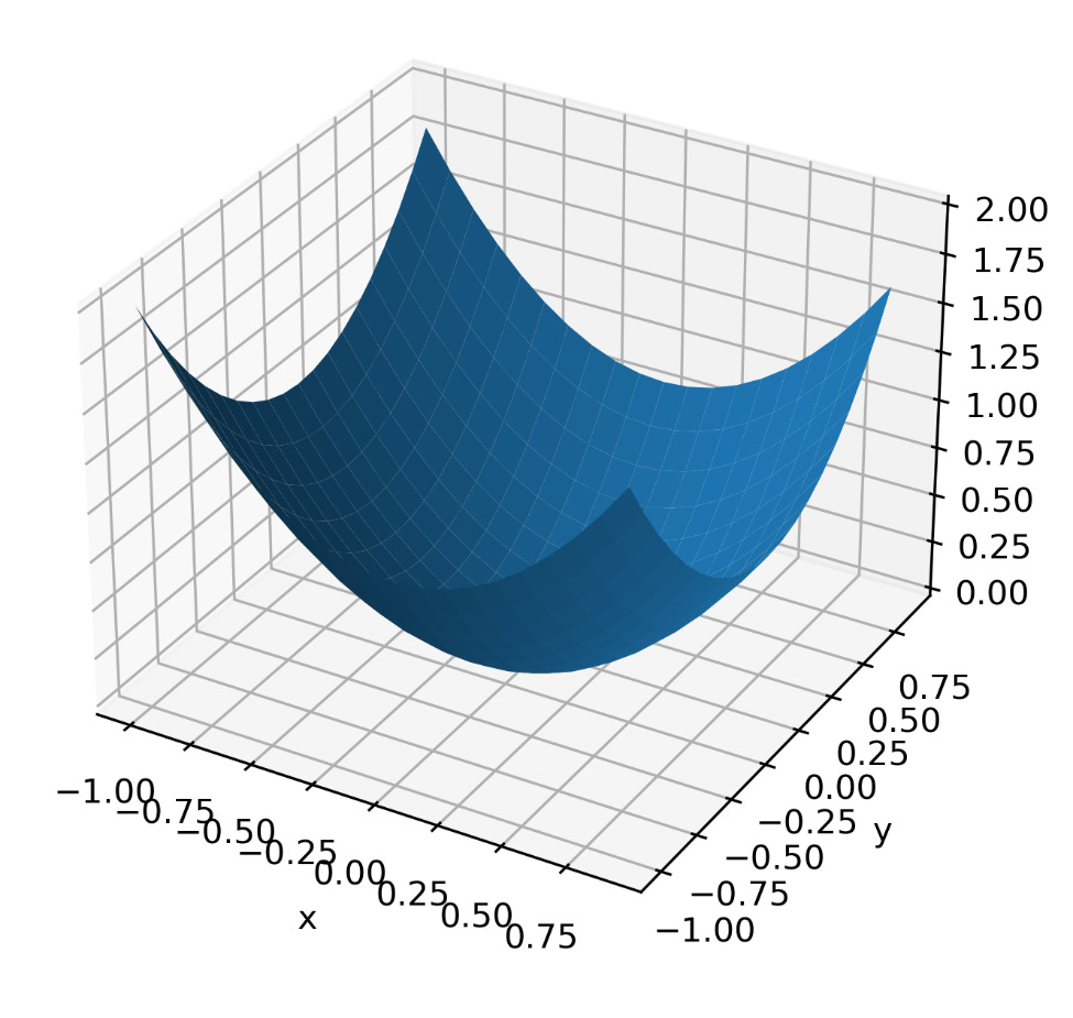

The following graph is shown:

Figure 8.5 – A function of two variables obtained using symbolic regression

3. Now, let’s generate the data we will use to derive the mathematical model:

   input_train = np.random.uniform(-1, 1, 200).reshape(100, 2)

   output_train = input_train[:, 0]**2 + input_train[:, 1]**2

   input_test = np.random.uniform(-1, 1, 200).reshape(100, 2)

   output_test = input_test[:, 0]**2 + input_test[:, 1]**2

We have generated two datasets. The first set (the train set) we will use to train the algorithm. This data will be used as starting data to evolve individuals until the convergence criterion is satisfied. The second set of data (the test set) will be used to evaluate the performance of the algorithm. To generate the input data, we used the numpy.random.uniform () function, which generates random numbers from a uniform distribution within a defined numeric range. The output was instead generated by applying the function of two variables, which is obtained by adding the squares of the two variables.

4. Now, we can set the parameters needed to perform symbolic regression:

   function_set = ['add', 'sub', 'mul']

   sr_model = SymbolicRegressor(population_size=1000,function_set=function_set,

                              generations=10, stopping_criteria=0.001,

                              p_crossover=0.7, p_subtree_mutation=0.1,

                              p_hoist_mutation=0.05, p_point_mutation=0.1,

                              max_samples=0.9, verbose=1,

                              parsimony_coefficient=0.01, random_state=1)

To start, we have defined the mathematical functions that will be exploited by the algorithm. We have limited the number of functions, since we already know what to look for; in practice, it is appropriate to foresee all the functions and then exclude those that appear inconsistent. The more functions that are provided, the larger the solution search domain will be. Next, we used the SymbolicRegressor() function from the gplearn library, which extends the scikit-learn library to perform genetic programming with symbolic regression.

The following parameters are passed:

• population_size: The number of programs in each generation
• function_set: The functions to use when building and evolving programs
• generations: The number of generations to evolve
• stopping_criteria: The value required to stop evolution early
• p_crossover: The probability of performing crossover on a tournament winner
• p_subtree_mutation: The probability of performing subtree mutation on a tournament winner
• p_hoist_mutation: The probability of performing hoist mutation on a tournament winner
• p_point_mutation: The probability of performing point mutation on a tournament winner
• max_samples: The fraction of samples to draw from x to evaluate each program on
• verbose: The verbosity of the evolution-building process
• parsimony_coefficient: The constant that penalizes large programs by adjusting their fitness to be less favorable for selection
• random_state: The seed used by the random number generator

5. Now, we can train the model:

   sr_model.fit(input_train, output_train)

Since we have requested to view the evolution of the procedure, we will see the following data printed on the screen:

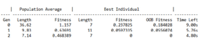
Figure 8.6 – The evolution of the symbolic regression procedure

Finally, we just have to print the results on the screen:

print(sr_model._program)
print('R2:',sr_model.score(input_test,output_test))

The following results are returned:

add(mul(X1, X1), mul(X0, X0))
R2: 1.0

The rhyme line gives us a mathematical model. Note that the formula has been provided in symbolic format; we can, in fact, see the operators (add and mul) and the variables (X1 and X0). If we apply operators to variables, we can easily obtain the following formula:

R2 refers to the coefficient of determination (R-squared). R-squared measures how well a model can predict the data and falls between zero and one. The higher the value of the coefficient of determination, the better the model is at predicting the data. We got the maximum value, indicating that the mathematical model fits the data perfectly.

After analyzing in detail how to obtain a mathematical model from data using symbolic regression, let’s now examine the oldest computation models inspired by the physical world – CA.

Exploring the CA model

The first studies on CA were by John von Neumann in the 1950s and were motivated by his interests in the field of biology, with the aim of defining artificial systems capable of simulating the behavior of natural systems. If the self-reproductive process can be simulated with a machine, then there must be an algorithm that can describe the operation of the machine. The research was aimed at replicating models that were computationally universal. We wanted to study computational models that had the property of not distinguishing the computation component from the memory component. The interactions in a cellular automaton are local, deterministic, and synchronous. The model is parallel, homogeneous, and discrete, both in space and in time. The connection of CA with the physical world and their simplicity are the basis of their success in the field of simulating natural phenomena.

CA are mathematical models that are used in the study of self-organizing systems in statistical mechanics. In fact, given a random starting configuration, thanks to the irreversible character of the automaton, it is possible to obtain a great variety of self-organizing phenomena. CA are treated using a topological approach; this mathematical method considers automata as continuous functions in a compact metric space. Being complex systems, they refer to the second law of thermodynamics, according to which, given a microscopic and isolated physical system, it tends to reach a state of maximum entropy and, therefore, disorder over time. Microscopic, irreversible, and dissipative systems, or open systems that are allowed to exchange energy and matter with the environment, are allowed to evolve from a state of disorder to a more orderly one through self-organizing phenomena.

CA, therefore, mathematically reproduce physical systems through discrete space-time variables, whose measurements are limited to a limited set of values, which are also discrete. The cellular automaton evolves over time, producing a certain number of generations. A new generation replaces the previous one, which affects the values of the new variables. The mere fact that the values do not have a linear dependency relationship generates non-trivial automata. The formation of patterns in the development of natural organisms is governed by very simple local rules and could be well described by the adoption of a cellular automaton model. Each spatial unit of the lattice, forming a regular matrix, is accompanied by discrete values describing the types of living cells. Short-range interactions can lead to the emergence of varied genetic characteristics.

A cellular automaton is defined on an infinite regular grid of any size in which the shape of the cells is always the same. Each point of the grid is called a cell. At every instant, each cell of the grid is in a state among the finite possible states. Each cell is characterized by at least two states – in the simplest cases, 0 and 1, or true or false. At discrete time intervals, all cells simultaneously update their state, based on the state of a finite number of other cells called neighbors. Usually, the neighborhood of each cell contains all those that have a distance of less than a certain value. The rule applied by each cell to determine its next state is the same. The global evolution of a cellular automaton is the evolution of the overall configuration of the cell network. Each configuration is sometimes called a generation, if related to the evolution of the overall state of the cell network or a pattern. We can define CA that differ from each other by varying the number of dimensions of the grid, the set of states, and so on.

The overall behavior of the automaton, at the t + 1 instance, is the reflection of the state at the previous t instant and of the transition operation, which usually affects the state transition of all cells, in synchrony. The rules that influence the behavior of the single cell are called “local” and the comprehensive behavior is called “global”. The changes affect the generations and the so-called neighborhood (the cells present in the surroundings that mutually influence the behavior of the others). The starting configuration is called a “seed” and can be made up of a cell or a pattern of cells. The choice of the initial situation can be casual or linked to design choices.

In summary, a cellular automaton is defined by the following elements:

• Cell: Represents the minimum unit to define the 2D and 3D space. An unlimited network of cells can describe the universe.
• Cellular state: Describes the state, at t instant, of the considered space unit, which can be full or empty. The cellular state can be defined according to a project’s needs.

Game-of-life

An example of a cellular automaton is the one conceived by Conway, which takes the name of game-of-life. The grid is two-dimensional, and the cells are square. A cell can be alive (represented with a black square) or dead (represented with a white square) (see Figure 8.7). Each cell changes its state according to the state of the eight cells around it (the neighbors) and the following rules:

• A living cell dies if the number of living neighbors is less than two (death by isolation)
• A living cell dies if the number of living neighbors is greater than three (death from overcrowding)
• A dead cell becomes alive if the number of living neighbors is exactly three (birth) 1
• In any other case, a cell retains its state

We can see that the rules are quite simple, but the behavior of the configurations, surprisingly, is anything but trivial. Indeed, Conway has shown that it is undecidable whether a given pattern will eventually lead to a configuration in which all cells are dead.

A classification has been made to refer to the various classes of patterns that can be observed in a configuration of this cellular automaton. Some of them are proposed here:

• Still life: These are patterns that remain unchanged over time and are fixed points of an updating rule
• Oscillator: Temporally periodic structures that do not remain unchanged, but after a finite number of updates, they reappear identically and at the same point of the grid
• Spaceship: Patterns that, after a finite number of generations, are repeated identically but are translated into space
• Cannon: A pattern that, like an oscillator, returns to its initial state after a finite number of generations but that also emits spaceships

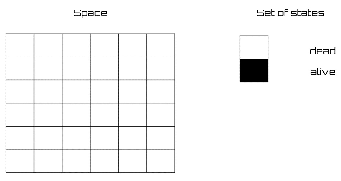
Figure 8.7 – A two-dimensional grid and states of the game-of-life CA

Note that many of the observed patterns were not designed ad hoc but emerged from initial random configurations. In fact, during the evolution of a pattern, the objects collide with each other, sometimes destroying themselves and sometimes creating new patterns.

Now, let’s see how to implement a simple example of a CA model in a Python environment.

Wolfram code for CA

Elementary CA models are, in a certain sense, the simplest CA that we can imagine (or almost). They have one dimension and each cell can be in one of two states; moreover, the neighborhood of each cell contains itself and the two adjacent cells. The only thing that distinguishes an elementary cellular automaton from the other is the local update rule. In general, it is possible to calculate the number of possible rules with s ^ (s ^ n), where s = number of states and n = number of neighbors (or, rather, of the cells taken into consideration, the neighbors plus the central node). In the case of elementary CA, s = 2 and n = 3, and then 2 ^ (2 ^ 3) = 2 ^ 8 = 256 elementary CA. Many of these are equivalent if you rename the states or swap left and right in cellular space. A common way of referring to an elementary cellular automaton is to use its Wolfram number. Wolfram proposed a classification of one-dimensional CAs with a few states and neighborhoods of a few cells, based on their qualitative behavior, and he identified four complexity classes (Wolfram classification):

• Class 1: CA that quickly converge to a uniform state after a defined number of steps.
• Class 2: CAs that quickly converge to stable or repetitive states. The structures are short-term.
• Class 3: CA evolving in states that appear to be completely random. Starting from initially different schemes, they create statistically interesting generations, comparable to fractal curves. In this class, the greatest disorder is perceived both globally and locally.
• Class 4: CA that form not only repetitive or stable states but also structures that interact with each other in a complicated way. At the local level, a certain order is observed.

Among the complexity classes, class 4 was particularly interesting due to the presence of structures (gliders) capable of propagating in space and time, so much so that it led Wolfram to put forward the hypothesis that the CA of this class may be capable of universal computation.

According to Wolfram, a rule is uniquely specified by the value it takes on each possible combination of input values – that is, by the following eight-bit sequence:

f (1, 1, 1), f (1, 1, 0), f (1, 0, 1), f (1, 0, 0),

f (0, 1, 1), f (0, 1, 0), f (0, 0, 1), f (0, 0, 0)

We can think of each bit as the state of the three cells adjacent to the next cell.

For example, consider the update rule of the next cell, 126. The 8-bit binary expansion of the decimal number 126 is 0111110, so the local update rule of the elementary cellular automaton with Wolfram number 126 is f, such that we get the following:

f (1, 1, 1) = 0, f (1, 1, 0) = 1, f (1, 0, 1) = 1, f (1, 0, 0) = 1,

f (0, 1, 1) = 1, f (0, 1, 0) = 1, f (0, 0, 1) = 1, f (0, 0, 0) = 0

So, if we consider the three adjacent cells, the next cell update rule will be like the one shown in Figure 8.8:

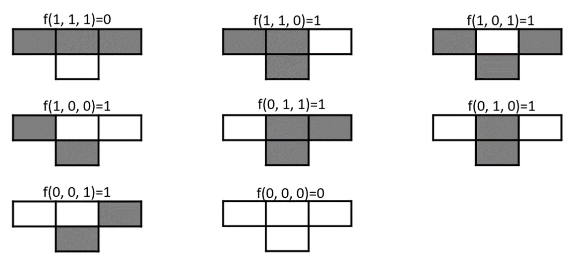
Figure 8.8 – Wolfram rules (126) of the updating cell state

The way to update the cells will then be indicated by these rules:

1. The first row at the top of the square grid will be initialized randomly.
2. Starting from these values, and following the rules indicated in Figure 8.8, the cells of the next row will be updated.
3. This procedure will be repeated until the last row of the grid is reached.

So, let’s move on to a practical example (cellular_automata.py). As always, we analyze the code line by line:

1. Let’s start by importing the libraries:

   import numpy as np

   import matplotlib.pyplot as plt

The NumPy library is a Python library that contains numerous functions to help us manage multidimensional matrices. Furthermore, it contains a large collection of high-level mathematical functions we can use on these matrices. The matplotlib library is a Python library for printing high-quality graphics. With matplotlib, it is possible to generate graphs, histograms, bar graphs, power spectra, error graphs, scatter graphs, and more using just a few commands. This includes a collection of command-line functions, such as those provided by MATLAB software.

2. Let’s now set the grid size and Wolfram update rules to follow:

   cols_num=100

   rows_num=100

   wolfram_rule=126

   bin_rule = np.array([int(_) for _ in np.binary_repr(wolfram_rule, 8)])

   print('Binary rule is:',bin_rule)

We first set the number of rows and columns of the grid (100 x 100). We then set up the Wolfram rule (126) that enforces the updates shown in Figure 8.8. Subsequently, we represented the Wolfram number in binary form; to do this, we used the NumPy binary_repr() function, which returns the binary representation of the input number as a string. Since we are interested in having a result in the form of an array of integers, we have also used the int (_) function, which converts the specified value into an integer number. Finally, we have displayed the result on the screen:

Binary rule is: [0 1 1 1 1 1 1 0]

The result is exactly what we expected and represents the 8-bit binary expansion of the decimal number 126.

3. Now, let’s initialize the grid:

   cell_state = np.zeros((rows_num, cols_num),dtype=np.int8)

   cell_state[0, :] = np.random.randint(0,2,cols_num)

We first created a grid of size (rows_num, cols_num) and then (100 x 100) and populated it all with zeros. We then initialized the first row, which, as previously mentioned, will contain random values. We used the NumPy random.randint() function, which returns an integer number’s selected element from the specified range. The randomly generated values will be only 0 and 1 and in a number equal to cols_num (100).

4. Now, let’s move on to update the status of the grid cells:

   update_window= np.array([[4], [2], [1]])

   for j in range(rows_num - 1):

       update = np.vstack((np.roll(cell_state[j, :], 1), cell_state[j, :],

                      np.roll(cell_state[j, :], -1))).astype(np.int8)

       rule_up = np.sum(update * update_window, axis=0).astype(np.int8)

       cell_state[j + 1, :] = bin_rule[7 - rule_up]

We first defined a window (update_window) that will allow us to obtain the cell update rule, starting from the state of the neighbors’ cells. We then updated the status of the cells row by row. We first retrieved the status of the three neighboring cells (left, center, and right) of the previous row immediately (update). So, we calculated the position of the update rule by calculating the sum of the states of the neighboring cells multiplied by the update window. The obtained number (0–7) will give us the position of the Wolfram sequence, as indicated here:

7 = f (1, 1, 1), 6 = f (1, 1, 0), 5 = f (1, 0, 1), 4 = f (1, 0, 0),

3 = f (0, 1, 1), 2 = f (0, 1, 0), 1 = f (0, 0, 1), 0 = f (0, 0, 0)

Finally, we retrieved the cell status in binary format from Wolfram’s update rules, simply subtracting from 7 the number obtained in the previous instruction (rule_up).

5. We just have to print the grid with the updated cell status:

   ca_img= plt.imshow(cell_state,cmap=plt.cm.binary)

   plt.show()

The following diagram is shown:

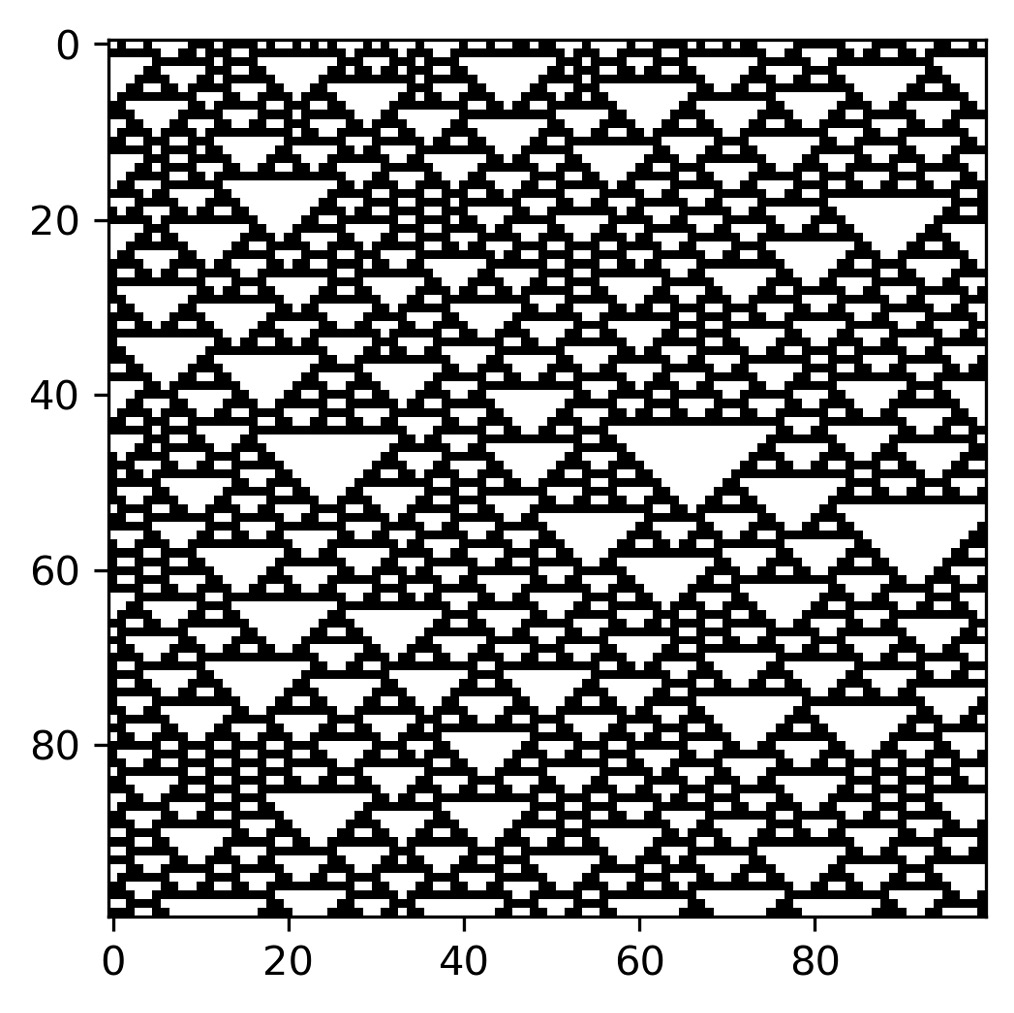
Figure 8.9 – The first 100 lines of the space-time diagrams of an elementary cellular automaton for Wolfram’s 126 class; the initial configuration is random

Rule 126 generates a regular pattern with an average growth faster than any polynomial model. It represents a special case by showing how chaotic behavior can be broken down into a wide range of figures: gliders, gliding guns, and still-life structures.

Summary

In this chapter, we learned the basic concepts of SC to exploit the tolerance of imprecision, uncertainty, and rough reasoning to achieve behavior like human decision-making. We analyzed the basic techniques of SC: fuzzy logic, neural networks, evolutionary computation, and GAs. We understood how these technologies can be exploited to support us in our choices. We then deepened the concepts behind GAs and saw how genetic programming based on human evolution can be valuable in the optimization of processes.

Subsequently, we learned how to use GA techniques to implement SR. Symbolic equations represent an important resource for scientific research. The identification of a mathematical model that can represent a complete system is far from an easy task. The use of data can come to our aid; in fact, through SR, we can discover the equation underlying a set of input-output pairs. After analyzing the basics of the SR procedure through genetic programming, we saw a practical case of SR for the identification of a mathematical model, starting from the data.

Finally, we explored the CA model, which is a mathematical model used in the study of self-organizing systems in statistical mechanics. Given a random starting configuration, thanks to the irreversible character of the automaton, it is possible to obtain a great variety of self-organizing phenomena. CA are treated using a topological approach. After analyzing the basics of CA, we learned how to develop an elementary cellular automaton based on Wolfram’s rules.

In the next chapter, we will learn how to use simulation models to handle financial problems. We will explore how the geometric Brownian motion model works, and we will discover how to use Monte Carlo methods for stock price prediction. Finally, we will understand how to model credit risks using Markov chains.