CHAPTER 6
Working with Data
In God we trust. All others bring data.
—W. Edwards Deming
Data is an essential component of analytics, and working with and understanding data is a critical analytical skill. Due to its nature, healthcare data is often more complex than that in other industries. Despite this complexity, many analytical tools such as dashboards and reports use simplistic (or even incorrect) approaches to analyze and represent the data. This chapter will focus on the key concepts behind understanding and effectively utilizing data. Covered are data type common to healthcare and how to select appropriate analyses for various data types so that healthcare information analysts are able to extract the maximum information and value from collected data.
Data: The Raw Material of Analytics
Data is the raw material of information. Data is continuously generated as healthcare professionals such as healthcare providers, administrators, and analysts use computerized systems as part of their jobs, or enter data into databases as part of post hoc data collection efforts for research, QI, or other reasons. The data that is stored in source-system databases, however, is rarely useful in and of itself. Just like any raw material, data must be processed in order to become useful. This processing is how data starts to become information that is useful for understanding the operations of a healthcare organization (HCO).
Figure 6.1 illustrates the information value chain. At the beginning of the chain is data, the raw material. The data is generated by electronic medical records and other computerized tools within healthcare. The next step in the chain is analysis, the step in which data is taken from its raw database form, summarized, and transformed into a more useful format. By applying the analysis and other processing available in analytics tools, the result is information and insight that is available to clinicians, administrators, and other information users. The intent is that this information helps to trigger actions, such as by implementing process improvements or assisting in clinical decision making, which in turn leads to improved outcomes that are in line with the quality and performance goals of the HCO.
FIGURE 6.1 Information Value Chain

When someone who is working on a healthcare QI project asks for data, the request is in fact rarely for just data. That is, someone would normally not be asking for a dump from the database unless that person is planning to do his or her own analysis. Requests for data usually stem from the need for information to help understand a problem, identify issues, or evaluate outcomes. Even simple summarizations of data (including counts, averages, and other basic statistics) begin the process of turning raw data into something that is more useful—information and insight that can be used for decision making and taking action.
Preparing Data for Analytics
It is important to fight the urge to dive into a new data set or newly added data elements without obtaining a clear understanding of the context of the data, and how it relates to the business. When developing analytics to address a need for insight and information around a quality or performance improvement initiative or issue, requisite information that an analyst needs to know includes:
- What the data represents. What process, workflow, outcome, or structural component does the data correspond to?
- How the data is stored. What kind of storage is the data in (such as an enterprise data warehouse), how is the data physically stored on the database, and how might that storage format constrict what can be done with the data? Also, how good is the quality of the data; are there missing values that might bias analysis, and are there invalid entries that need to be cleaned and/or addressed?
- The data type. Regardless of how data might be physically stored in a database, what kind of data do the values represent in “real life”?
- What can logically be done with the data. Given the type of data and how it is stored, what kind of database and mathematical operations can be performed on the data in meaningful ways?
- How can the data be turned into useful information that drives decision making and enables leaders and quality stakeholders to take appropriate and necessary action?
When analysts begin working with a new data set, they should spend time on the floor (or elsewhere in the HCO) where the activity occurs that generates the data, and where the resultant analytics insight is used. This hands-on exposure helps relate data to actual situations and conditions and provides invaluable context to existing documentation and metadata.
Understanding What Data Represents
At the heart of successful quality and performance improvement in healthcare is modifying existing and creating new business and clinical processes that reduce waste, are more effective, and reduce the likelihood of medical errors. To be useful for quality and performance improvement, data must be analyzed within the context of the processes and workflows through which it is originally generated. This section will focus on the methods for aligning data to processes and using that data as a basis for analytics.
Aligning Processes with Data
Clinical processes and workflows have been in place since the advent of modern medicine; enterprise data warehouses and clinical software applications are much more recent inventions. It is not surprising, then, that until very recently, the people primarily concerned with the processes of healthcare were not the same people whose primary concern is the data generated by those processes. Because healthcare systems are dynamic, processes are constantly changing; stewards of healthcare data are often not informed of such changes, or may not be able to keep up with the changes in processes occurring on the front line.
To provide accurate insights, analytics must use data that is representative of what is actually happing on the front lines. For this reason, analytics professionals must work very closely with business subject matter experts who are able to convey the most recent process changes and validate that the current assumptions on which analytics is based match what is occurring on the front line.
Figure 6.2 represents, at a high level, the steps necessary for a patient to be seen by an emergency department physician. Each of the steps in the process represents its own activities (such as triaging a patient), requires a specific resource (such as a registration clerk, nurse, or physician), and generates its own data (via interactions with clinical software). See Table 6.1 for a sample of the type of data that would be typically generated in a process such as the one illustrated in Figure 6.2.
FIGURE 6.2 Sample Emergency Department Patient Arrival and Assessment Process
TABLE 6.1 Context Details of an Emergency Department Patient Arrival and Assessment Process
| Process Step | Description | Data |
| Triage | Nurse performs a preliminary triage assessment of the patient to determine his or her presenting complaint and the urgency of the patient’s condition. | Arrival time Mode of arrival (ambulance, car, etc.) Time triage started Time triage completed Triage acuity score (1 through 5) Presenting complaint Vital signs |
| Patient arrival | Registration clerk registers patient and collects full demographic and billing information. | Time registration started Time registration completed Full patient demographic and insurance information |
In addition to knowing which process a data item is associated with, other important information to note about each data point includes:
- Who performs the activity that generates the data?
- Who enters the data element into the system (in the case an observation or similar data) or causes data to be generated (through some other interaction with a clinical system such as changing a status code)?
- What is the trigger for the data to be stored?
- What type of data is stored (such as numeric, alphanumeric, and date/time)?
- What business and validation rules are associated with the data item?
- What data is required to provide the information and insight required to address the quality and performance goals of the organization?
Types of Data
Data can be divided into two basic types: quantitative or numeric, and qualitative or nonnumeric.1 Quantitative data typically is obtained from observations such as temperature, blood pressure, time, and other similar data. Qualitative data, on the other hand, tends to be more descriptive in nature, and may consist of observations and opinions (entered into an electronic medical record), patients’ experiences while receiving care, transcribed notes from focus groups, or researchers’ notes. Quantitative data is easier to summarize and analyze statistically; qualitative data usually requires more preparation prior to analysis, but can reveal insights into quality and performance that standard quantitative analysis cannot pick up.
Improvement science identifies three types of data: classification, count, and continuous.2 Classification and count data are sometimes collectively referred to as attribute data, and continuous data likewise is often referred to as variable data. Attributes associated with classification data are recorded as one of two classifications or categories, such as pass/fail, acceptable/unacceptable, or admitted/nonadmitted. Count data, as would be expected, is used to document the number of occurrences of typically undesirable events or outcomes, such as number of central line infections, falls from hospital beds, critical incidents, and other occurrences related to quality and performance. Finally, continuous data is often associated with productivity or workload, such as emergency department census, X-rays performed, wait times, and other measures of performance.
Once an understanding is obtained of what the data means in “real life” (that is, how the data is mapped to processes, workflows, and other aspects of healthcare delivery), the data needs to be understood in terms of what type of data it is (once again in “real life”) versus how it is stored and formatted on an electronic database. Knowing this allows analysts and developers to create meaningful analyses of the data; if the type of analysis performed on data is not appropriate, the results may in fact be nonsensical, as the following examples will illustrate.
ELECTRONIC STORAGE OF DATA
People who are familiar with programming languages or databases will know that data can be classed in many ways based on what is being stored. In a database, for example, the data type assigned to a field (or object) typically will define four main attributes of what is to be stored in that field (or object).3 These four main attributes (at the database level) consist of:
At the database level, the data type that is assigned to a field controls what kind of information can be stored in that field. This helps to ensure the integrity of data stored so that when the data is read back from the database, the software knows how to interpret the data being loaded. See Figure 6.3 for a sample screenshot from a database program illustrating various data fields and how their type is encoded.
FIGURE 6.3 Screenshot of Database Showing Data Fields and Data Types
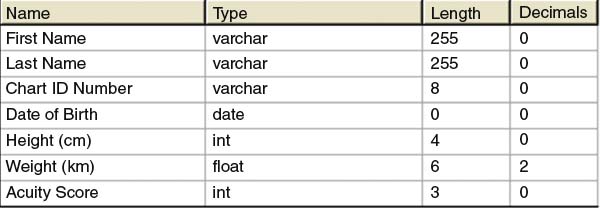
Data types in a database ensure the integrity and management of the information stored on the database. The data type assigned to a database field also dictates what operations can be performed on the data in that field. For example, typical mathematical operations (such as multiplication and division) cannot be applied to character-type data, so multiplying a patient’s name by a number (or multiplying two names together) would be an illegal operation. Databases (and analytical software) typically strongly enforce these rules so that inappropriate operations cannot be performed.
A challenge arises, however, if data is coded in a database as an inappropriate type. Attributes of data from a computer database may not always accurately relay what analysis truly makes sense to perform on data. For example, I have seen numeric temperature values such as 37.0 stored in text-type data fields because the programmers wanted to store the entry as “37.0 degrees Celsius” to ensure the unit of measure was captured with the temperature (even though a temperature is clearly numeric and can be treated as such). When this occurs, data type casting (that is, converting from one data type to another) and other manipulations may be necessary to allow for the desired operations to be permissible. In this case, the “degrees Celsius” would need to be stripped from the data, and the resultant values type cast to a numeric value so that graphing, summarizations, and other calculations become possible with the temperature data.
In summary, know your data and beware of treating data strictly as specified in database attributes without first knowing the context of the data, what it really means, and what data summarizations and analyses must be performed.
LEVELS OF MEASUREMENT
Data is stored in a database using data types that best approximate the type of data the field represents. In Figure 6.3, for example, the “Chart ID Number” is stored as a “varchar” type, which is a field that can hold both letters and numbers. Chart numbers are typically numeric (such as 789282), but may include non-numeric characters (such as 789282–2 or AS789282), so a character format may be necessary to accommodate such non-numeric values. Also in Figure 6.3, height (in centimeters) and weight (in kilograms) are stored in numerical formats (integer and floating-point, in this instance), and the “Acuity Score” is stored as an integer.
Regardless of how data is (correctly or incorrectly) stored in a database, every observation has a “true” data type that, depending on the context and the meaning of the data, dictates what types of analysis or computation are meaningful to perform with that value. From a scientific point of view, there are four generally accepted classes of data (or levels of measurement). The four classes of data according to traditional measurement theory consist of categorical (or nominal), ordinal, interval, and ratio.4 See Table 6.2 for a summary of these four basic levels of measurement.
TABLE 6.2 Classes of Data (Levels of Measurement)
| Data Type | Description |
| Categorical (Nominal) | Non-numeric data that is placed into mutually exclusive, separate, but non-ordered categories. |
| Ordinal | Data that may be categorized and ranked in a numerical fashion, and for which order matters. The difference between values is not meaningful nor consistent. |
| Interval | Data that is measured on a scale where the difference between two values is meaningful and consistent. |
| Ratio | Measurement where the difference between two values is meaningful and consistent, and there is a clear definition of zero (there is none of that variable when it equals zero). |
CATEGORICAL AND ORDINAL DATA
Any values that are mutually exclusive (in that they cannot belong to more than one category) and do not follow a specific order can be considered categorical data. An example of categorical data is a patient’s gender, typically either female or male. Another example of categorical data is location or bed number. In Figure 6.4, the top set of ovals represents emergency department locations (“Resus 1,” “Resus 2,” “Waiting Room,” etc.) and can be considered categorical in nature. These fit the criteria of categorical data because there is no implicit order and the categories are mutually exclusive.
FIGURE 6.4 Illustration of Categorical and Ordinal Data
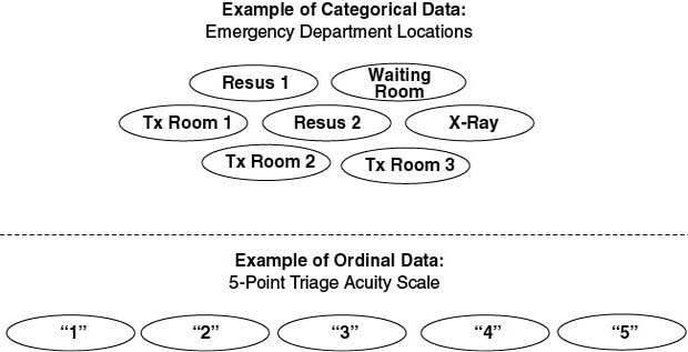
Ordinal data is similar to categorical data in that it is groupings, except that the order of the values does matter. Consider, for example, the bottom set of ovals in Figure 6.4, which represent triage acuity scores. In the example, the triage acuity scores are on a 5-point scale (1, 2, 3, 4, 5) where 1 represents the sickest patient whereas 5 is the least sick. In this case, the order of the values implies a level of illness, but the difference in illness between a 1 and a 2 is not the same as that between a 2 and a 3, and so on. In the example, and all ordinal data, the actual differences between the numbers have no meaning except to imply an order; in this case, the acuity scale could have just as easily been A through E.
INTERVAL AND RATIO DATA
Values that are mere categories or groupings are good for counting, but not very good for measuring—that is where interval and ratio values are important. Intervals and ratios are where “real” analysis becomes possible, because the difference between any two interval or ratio values is both meaningful and consistent. The difference between interval and ratio values, however, is that there is a clear definition of zero in ratio values. Take the example of temperature (illustrated in Figure 6.5). Both Celsius and Fahrenheit temperature scales include zero degrees, but zero degrees Fahrenheit and Celsius do not represent an absence of temperature (although it might feel like it!); temperature values are regularly recorded in negative values as part of the scale. The Kelvin temperature scale, however, is considered a ratio because “absolute zero” (zero degrees K) means the total absence of temperature.
FIGURE 6.5 Illustration of Interval and Ratio Values Using Temperature as an Example

Most measurements that are taken in physical sciences, engineering, and medicine are done on a ratio scale. For example, readings for mass (pounds or kilograms), time (seconds, hours), and blood glucose (mmol/L) all start at zero, which represents an absence of that quantity.
Getting Started with Analyzing Data
Analysis of data is, of course, the heart of healthcare analytics. Developing analytics strategies, building data warehouses, and managing data quality all culminate with analyzing data and communicating the results. Data analysis is the process of describing and understanding patterns in the data to generate new information and new knowledge that can be used for decision making and QI activities.
One might ask why it is important to delve into how data is stored on a database and how it is related to categorical, ordinal, interval, and ratio levels of measurement. The bottom line is that before we perform any operations on data we have, we need to know what operations make sense to perform. Analyzing data properly, and obtaining meaningful results from analytics, requires that we know what kind of data we are dealing with. If we perform operations on data that fundamentally do not make sense in relation to the type of data we’re working with, then any outputs from (and inferences made based on) those analytics will be faulty.
Just looking at data in a database is not very helpful—usually “something” needs to be done with the data, such as summarizing it in some way, combining it with other data, among other possible operations. The type of information that data represents ultimately determines what computations can be performed with it.
Summarizing Data Effectively
There are many uses for data, including to evaluate the outcome of a QI project, assist in clinical decision support, or gauge the financial health of an HCO to name a few. Regardless of how data is used, the strength of and value derived from analytics is the compilation and analysis of large amounts of data and resultant synthesis of a meaningful summary or insight from which clinicians, administrators, and QI teams can base decisions and take meaningful, appropriate action.
It seems as though dashboards are becoming nearly ubiquitous throughout HCOs. This is because the visualization techniques used in well-designed dashboards provide an “at-a-glance” overview of performance. Most dashboards used in the management of healthcare require, at the very least, basic summaries of data such as count (frequency), average, or range. More sophisticated uses of information (such as are common in quality and performance improvement) may require more advanced operations to be performed with the data.
Table 6.3 is an overview of common data summary approaches along with the types of data for which each of the summaries is appropriate. As a point of clarification, when we are describing a population of patients, the term for the values describing the population is “parameters,” whereas “statistics” is the term for the descriptive characteristics of a sample.
TABLE 6.3 Overview of Data Summaries
| Summary | Description | Applies To |
| Count | A tally of all the values (or ranges of values) in a sample of data. | Nominal, ordinal, interval, ratio |
| Mode | The most commonly occurring value in a data set. | Nominal, ordinal, interval, ratio |
| Percentile | The value in a data set below which a specified percentage of observations fall. | Ordinal, interval, ratio |
| Median | The “midway” point of a ranked-order data set; the value below which 50 percent of the data elements sit. Also known as the “50th percentile.” | Ordinal, interval, ratio |
| Minimum | The lowest value in a data set. | Ordinal, interval, ratio |
| Maximum | The highest value in a data set. | Ordinal, interval, ratio |
| Summary | Description | Applies To |
| Mean | The arithmetic average of a data set calculated by adding all values together and dividing by the number of values. | Interval, ratio |
| Variance | A measure of how spread out the numbers are within a data set and is measured by a value’s distance from the mean. | Interval, ratio |
| Standard deviation | Provides a sense of how the data is distributed around the mean and can be considered an average of each data point’s distance to the mean. | Interval, ratio |
COUNTING
Counting data is perhaps the most simple operation that can be performed, yet it is one of the most common and useful ways to look at data. A few of the most common questions asked by healthcare managers and executives is “how much” or “how many”—“How many central line infections occurred last week?” or “How many patients are now in the waiting room?” or “How many influenza patients can we expect to see during next flu season?” Many quality and performance initiatives are concerned with reducing the number of something (such as medication errors, unnecessary admissions, or patients exceeding length-of-stay targets) or increasing the number of something (such as patients answering “excellent” on a satisfaction survey). Accurate counts are an essential component of baseline data, and can assist in profiling data for data quality management efforts.
Counts of data appear on almost every performance dashboard and management report, and can figure prominently in the development of predictive models. Two common ways to report counts of variables include frequency distributions and histograms.
FREQUENCY DISTRIBUTION
Before working in depth with data, it is important to get an overall sense of what the data “looks like” to have a better idea of what statistical approaches might be appropriate. A frequency distribution is a count of occurrences of one or more of the values (or ranges of values) that are present in a sample of data.
There are many uses for frequency distributions in healthcare quality and performance improvement. These include counting (for example, the number of surgical procedures performed, by procedure code, and at a certain hospital site) and understanding the “spread” of the data, or how tightly clustered it is. For example, a tabulation of the number of surgeries performed in each of a hospital’s operating theaters over a specified time period could be illustrated in a frequency distribution. Frequencies are also invaluable for identifying limitations in the data and highlighting cleaning needs. For instance, frequency distributions can be used for determining the percentage of missing values and invalid data entries in a sample of data.
A frequency distribution can display the actual number of observations of each value, or the percentage of observations. Frequency distributions are very flexible, in that they are appropriate for all types of data values (categorical, ordinal, interval, and ratio), so no other mathematical operation is required other than counting (and calculating a percentage).
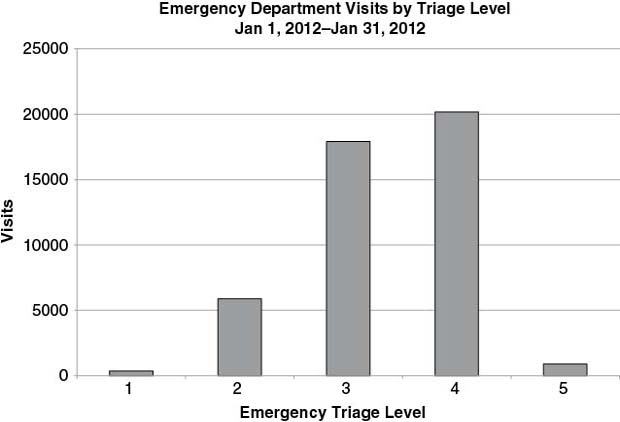
See Table 6.4 for a sample frequency distribution of emergency department visits by triage level. Note that in this case, triage level is ordinal data—the order matters (ranging from 1 being the most acute to 5 being the least acute), but the difference between the numbers does not.
TABLE 6.4 Sample Frequency Distribution (Emergency Department Visits by Triage Level)
| Triage Level | Visits (n) | Percent (%) |
| 1 | 364 | 0.80% |
| 2 | 5, 888 | 13.02% |
| 3 | 17, 907 | 39.58% |
| 4 | 20, 177 | 44.60% |
| 5 | 904 | 2.00% |
With the data graphing capabilities that are available in even the most basic data analysis tools, it is very rare to see a frequency distribution table without some graphic representation. Many people are able to grasp data better through visual representation, and differences in values can often be highlighted more effectively in a graphical format than can be done with a simple table.
Bar graphs and line graphs are two very common ways to visualize frequency data. See Figure 6.6 for a bar graph of the frequency distribution shown in Table 6.4. Notice how the graph clearly shows the large number of visits triaged as 3 and 4 compared to other triage scores. If the triage scale is such that 1 is the most acute and 5 is the least acute, then it is clear by Figure 6.6 that the emergency department represented in the graph sees many more patients that are mid-to-low acuity than highly acute patients.
FIGURE 6.6 Frequency Distribution of Emergency Department Visits by Triage Level
HISTOGRAM
Sometimes a detailed picture of how data is distributed throughout its range is necessary to answer questions such as: Do the values cluster around some single value? Are there many outliers? and What is the overall “shape” of the data? To help answer these questions, a histogram is used. A histogram is a specialized form of graph that is used to display the distribution of a set of data over its range (or sometimes a portion of the range). More formally, a histogram is an estimate of the probability distribution of a continuous variable (that is, a variable for which any value is possible within the limits of the variable’s range).
See Figure 6.7 for a sample histogram drawn from emergency department lengths of stay. A histogram is constructed by placing a series of adjacent bars over discrete intervals in a range of data; the height of each bar represents the frequency of observations within that particular interval. A histogram can be made more or less detailed by changing the size of the bin that each bar represents. From the histogram in Figure 6.7, it is possible to see that the majority of lengths of stay fall roughly between 0 and 5 hours, and that there are a number of outliers that stay up to 24 hours. The main difference between the histograms in Figure 6.7(A) and Figure 6.7(B) is that (B) is divided into 30-minute intervals compared to 60-minute intervals in (A). In summary, a histogram can be used:
FIGURE 6.7 Histogram of Emergency Department (ED) Length-of-Stay Values
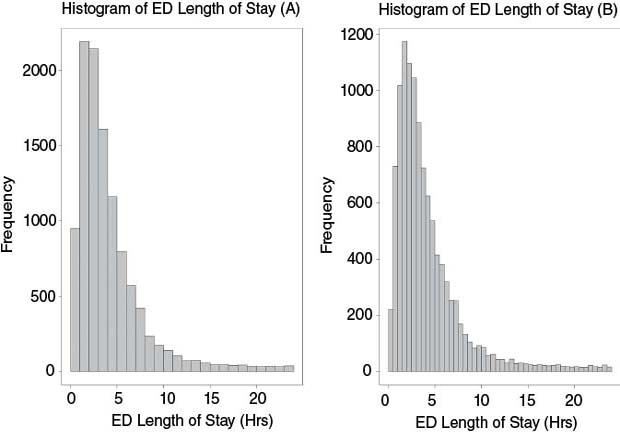
- When data are numerical.
- To observe the shape of the distribution of data.
- To determine the extent to which outliers exist in the data.
Knowing the shape of a distribution can reveal important details about the data and the processes from which the data was generated.6 For example, a shape that resembles the normal distribution or “bell curve,” in which data points are as likely to fall on one side of the curve as the other, suggests that the underlying process may be in control, exhibiting expected natural variation. Some statistical tests can only be performed on a data set that is normally distributed. A skewed distribution is asymmetrical, leaning to the right or to the left with the tail stretching away, because some natural limit prevents outcomes on one side. For example, histograms of length of stay (such as Figure 6.7) are very often skewed to the right (meaning the tail stretches to the right) because lengths of stay cannot be less than 0. Another common distribution observed in a histogram is bimodal, which shows two distinct peaks. A bimodal distribution suggests that the sample may not be homogeneous, and perhaps is drawn from two populations. For example, a histogram for lengths of stay that included both admitted and nonadmitted emergency department patients may exhibit a bimodal tendency, with one peak occurring for the shorter lengths of stay for nonadmitted patients and another peak from the lengths of stay of admitted patients.
Central Tendency
When you look at values associated with a quantitative variable (such as length of stay), the values are not usually spread evenly across the range of possible values, but tend to cluster or group around some central value. This is called central tendency. A measure of central tendency, then, is an attempt to describe data as accurately as possible, using a single value that best describes how data tends to cluster around some value.
The three most common measures of central tendency are the mean (or average), the median, and the mode. When a healthcare administrator or QI team member asks for a summary of a set of data, one of these (or typically both the mean and median) is usually what is implied. See Figure 6.8 for an example of how the measures of central tendency may fall on a fictional distribution of data.
FIGURE 6.8 Measures of Central Tendency
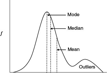
The average (or mean) is probably one of the most commonly used methods to summarize data, but it may also at times be misused. In essence, the average is calculated by summing up all the values of a variable in a set of data and dividing by the total number of observations. Average is a standard calculation on nearly every software tool that manages or manipulates data, so is typically the default summary of data. There are a few key points to remember when using averages. First, not all seemingly numeric data can be averaged; average is only appropriate for ratio and interval data (such as time, weight, temperature, and other physical observations). If a 5-point triage scale is in use, it would never make sense to say, “Our average triage acuity score was 3.4 today.” (An alternative, however, would be to say, “Over 50 percent of our cases were triaged at level 3 or higher.”)
Another issue with mean is that it is susceptible to outliers. If all observations in a data set tend to cluster around the same set of values, then average may be an accurate representation of that clustering. The average, however, can be skewed by small numbers of observations at extreme ends of the range of values. For example, if the typical hospital stay is between two and three days, the average of all observations can be skewed upward by even relatively few numbers of patients with extreme lengths of stay (say 30 days or more). See, for example, in Figure 6.8 that there is a group of outliers in the upper value ranges of the x axis, and as a result the mean is skewed to the right (that is, it is made to be larger).
There are other ways to summarize data either in conjunction with or instead of mean if the data is likely affected by outliers or is not a ratio or interval type. The alternative is to use the median (and percentile values). In essence, a percentile is the particular value in a set of data below which a certain percentage of the observations in a data set are located. For example, in a sample set of data, the 25th percentile is the value below which 25 percent of the values fall. Likewise, the 90th percentile is the value in the set that 90 percent of the samples lie below. The median is a specific instance of a percentile—it is the name given to the 50th percentile; in a data set, half of the observations of a particular variable will be below the median value, and the other half above it. In Figure 6.8, the median is much closer to the main clustering of observed values than is the mean due to the effect of the outliers. Figure 6.8 also illustrates the mode, which is the value in the data set that occurs the most frequently. Interestingly, I have never been asked for the mode of a data set directly, but rather I get asked for “mode-like” information, such as “What is the triage acuity with which most patients present,” “What time of day do we see the most patients walk in the door,” and “What is the most commonly ordered diagnostic test.”
Median and percentiles are valuable measures of central tendency in healthcare because they are not impacted by extreme outliers in a data set. In addition, median and percentiles can be calculated for ordinal, interval, and ratio data types. (They do not apply to categorical data because there is no implied order in the categories.)
The Big Picture
It is seldom a good idea to report complex healthcare performance parameters as a single value. For example, what does an average hospital length of stay of 4.9 days really mean? Judging from that number alone, it can mean anything from almost all patients staying nearly exactly five days to half of the patients staying less than one day and the other half of patients staying 10 days. While neither of these scenarios is particularly likely, it is impossible to discern what the true distribution of patient lengths of stay looks like from a single value.
Given the current capabilities of even relatively inexpensive analytical tools (not to mention some exceptional capabilities in open-source software), there is no excuse for not presenting information in a comprehensive manner that provides a more complete picture of quality and performance within the HCO. Just as it would be absurd for a pilot to navigate a plane based on “average airspeed” or “median altitude,” it is now up to HCOs to guide clinical, administrative, and QI decision making with data that is more comprehensively and accurately summarized (and in ways that make the data easier to understand).
Consider a data set containing three months of visit data for a midsized emergency department during which time there were 11, 472 visits. Providing just a few basic statistics can help to provide a more complete picture than a single statistic alone; when combined with a graph, the result is even more helpful. The three-month performance of our midsized emergency department can be summarized in Table 6.5.
TABLE 6.5 Summary of Three Months of Emergency Department Length-of-Stay Data
| Statistic | Value (hours) |
| Average | 4.86 |
| Median | 3.25 |
| Maximum | 23.97 |
| 25th percentile | 1.88 |
| 75th percentile | 5.68 |
| 90th percentile | 10.37 |
In Table 6.5, the average length of stay (LOS) is 4.86 hours whereas the median LOS is 3.25 hours. Table 6.5 also indicates that 75 percent of the visits had an LOS of 5.68 hours or less, and 90 percent of the LOS values were at 10.37 hours or less. What do these basic statistics tell us about the LOS data? Since the median is the midpoint of the data (or the 50th percentile) and the average at 4.86 hours is 1.61 hours greater than the median, with the value at the 90th percentile (10.37 hours) being almost twice that of the 75th percentile, those differences tell us that the data, in some way, is skewed. (If the data was tightly clustered around the mean, there would be very little difference between the mean and the median.) Judging from the values alone, it is possible to determine that although 75 percent of the visits experience an LOS of 5.68 hours or less, 25 percent are in fact greater than 5.68 hours and 10 percent are greater than 10.37 hours. While these values when used in concert provide a better overview of LOS performance than a single statistic (such as average) used alone, there is nothing really “actionable” in this data, and there are no real clues as to where to begin looking for opportunities for improvement.
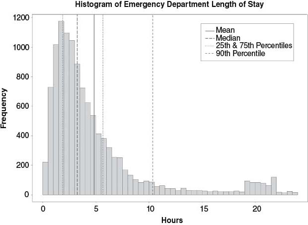
When the statistics in Table 6.5 are combined with an appropriate visualization of the LOS data (such as a histogram) as in Figure 6.9, the picture becomes more complete. With the visualization, users of the information can see that indeed the majority of emergency department visits are between 0 and 6 hours, but also that there are considerable numbers of visits between 6 and 24 hours. One thing that the data in Table 6.5 did not indicate is the small cluster of outliers around the 20-hour mark. Whether this group of outliers around 20 hours is indeed an issue and worthy of further investigation will require additional analysis of the data. The point is, however, that without a more thorough summarization of the data (using multiple statistics and appropriate visualization), this potential opportunity for improvement might not have been noticed.
FIGURE 6.9 Histogram of Emergency Department Length of Stay with Measures of Central Tendency
Another very useful way to summarize data is to use a box-and-whisker plot. Box-and-whisker plots present a very concise summary of the overall distribution of a given variable within a data set.7 Figure 6.10 is an example of a box-and-whisker plot; in a single graphical element, the box-and-whisker plot illustrates:
FIGURE 6.10 Example Box-and-Whisker Plot

The bottom and the top of the box in this type of plot always represent the first and the third quartiles, and the band within the box always represents the median. There are some variations in the way the lower and upper extremes, or the whiskers, can be plotted. Some common variations include where the ends of the whiskers represent:
- One standard deviation above and below the mean of the data.
- 1.5 times the interquartile range.
- The minimum and maximum of all data in the data set.
In fact, the whiskers of a box-and-whisker plot can represent almost any range that suits the particular needs of an analysis as long as the specified range is clearly labeled on the plot. When data exists that does not fall within the specified range of the whiskers, it is customary to individually plot those outlier data points using small circles.
Box-and-whisker plots are helpful to compare the distributions between two or more groups to help determine what, if any, differences in performance or quality may exist as exhibited by variations in their data. For example, even though two subgroups of data may exhibit similar characteristics (such as mean or median), a box-and-whisker plot helps to determine the presence of any outliers in any of the groups, and how the overall spreads in the data compare. Figure 6.11 illustrates emergency department LOS data graphed in a box-and-whisker plot broken down by acuity level. In Figure 6.11, it is possible to see how the different subgroups (triage acuity level) differ in their medians and spread, suggesting that these patient subgroups follow different trajectories during their emergency department stay.
FIGURE 6.11 Box-and-Whisker Plot of Emergency Department Length-of-Stay Data Broken Down by Triage Acuity

Scatter plots are used to determine if there is a correlation or relationship between two variables.8 For example, Figure 6.12 is a scatter plot with emergency department time “waiting to be seen” (WTBS) by a physician on the x axis and “left without being seen” (LWBS) on the y axis. By plotting the two variables against each other on the graph, it is possible to see the direction and strength of their relationship (if any). Figure 6.12 shows that there is a positive, but somewhat weak, and generally linear correlation between WTBS and LWBS when daily averages of LWBS and WTBS were compared; this makes intuitive sense, since the longer people need to wait for a doctor in the ED, the more they are likely to leave and seek treatment elsewhere. The more defined the trend is on the graph, the stronger the relationship (either positive or negative); the more scattered the plotted values are, the weaker the relationship.
FIGURE 6.12 Scatter Plot of Left without Being Seen Rates and Emergency Department Length of Stay

Scatter plots are often the starting point for more advanced analytics. Scatter plots often may provide a clue that a relationship between two (or more) variables does exist and that it may be possible to model that relationship and use it for predictive purposes.
Data summarized in ways similar to those described in this section is more complete, more useful, and more likely to provide actionable insight than a single statistic or high-level summary, yet does not require significantly more statistical literacy on the part of the consumers of the information.
I am not advocating that every dashboard, report, and other analytical tool must be loaded with as much context and information as possible; this would indeed lead to information overload. The purpose of these examples is merely to illustrate that because many quality and performance problems in healthcare are complex, the more ways that a problem or issue can be broken down and analyzed, the more likely it is that opportunities for improvement will be identified and that changes in quality and performance can be detected and evaluated. That is, after all, what I believe healthcare analytics is really about.
Summary
In my experience developing analytics for quality and performance improvement, I have rarely needed to rely on much more than these descriptive statistics to effectively communicate and identify process bottlenecks, performance changes, and overall quality. I believe it is much more important to focus on getting the data right, and focus on getting the right metrics that truly indicate the performance of the organization, than using complex statistics to overcome poor data quality and/or looking for a signal in the noise when there is no real signal in the first place. I have seen many analysts bend over backwards trying to use statistics to look for a change in performance when in fact the data was not good enough to answer the question that was being asked. Statistical analysis should never be a substitute for good data, for well-defined metrics, and should never be used to look for something that is not there.
Notes
1. Lloyd P. Provost and Sandra K. Murray, The Health Care Data Guide: Learning from Data for Improvement (San Francisco: Jossey-Bass, 2011), Kindle ed., location 1431.
2. Ibid., locations 1480–1481.
3. Microsoft Developer Network (MSDN), “Data Types (Database Engine),” http://msdn.microsoft.com/en-us/library/ms187594(v=sql.105).aspx.
4. Provost and Murray, The Health Care Data Guide, location 1496.
5. Glenn J. Myatt, Making Sense of Data: A Practical Guide to Exploratory Data Analysis and Data Mining (Hoboken, NJ: John Wiley & Sons, 2007), Kindle ed., location 641.
6. ASQ, “Typical Histogram Shapes and What They Mean,” http://asq.org/learn-about-quality/data-collection-analysis-tools/overview/histogram2.html.
7. Thomas H. Wannacott and Ronald J. Wonnacott, Introductory Statistics, 5th ed. (New York: John Wiley & Sons, 1990), 29.
8. Ibid., 478.