Chapter 6
Decompose It: Unpacking the Details
The everyday meanings of most terms contain ambiguities significant enough to render them inadequate for careful decision analysis.
—Ron Howard, Father of Decision Analysis1
Recall the cybersecurity analyst mentioned in Chapter 5 whose estimate of a loss was “$0 to $500 million” and worried how upper management would react to such an uninformative range. Of course, if such extreme losses really were a concern, it would be wrong to hide it from upper management. Fortunately, there is an alternative: Just decompose it. Surely such a risk would justify at least a little more analysis.
Impact usually starts out as a list of unidentified and undefined outcomes. Refining this is just a matter of understanding the “object” of measurement as discussed in Chapter 2. That is, we have to figure out what we are measuring by defining it better. In this chapter, we discuss how to break up an ambiguous pile of outcomes into at least a few major categories of impacts.
In Chapter 3 we showed how to make a simple quantitative model that merely makes exact replacements for steps in the familiar risk matrix, but does so using quantitative methods. This is a very simple baseline, which we can make more detailed through decomposition. In Chapter 4 we discussed research showing how decomposition of an uncertainty especially helps when the uncertainty is particularly great—as is usually the case in cybersecurity. Now, in this chapter we will exploit the benefits of decomposition by showing how the simple model in Chapter 3 could be given more detail.
Decomposing the Simple One-for-One Substitution Model
Every row in our simple model shown in Chapter 3 (Table 3.2) had only two inputs: a probability of an event and a range of a loss. Both the event probability and the range of the loss could be decomposed further. We can say, for example, that if an event occurs, we can assess the probability of the type of event (was it a sensitive data breach, denial of service, etc.?). Given this information, we could further modify a probability. We can also break the impact down into several types of costs: legal fees, breach investigation costs, downtime, and so on. Each of these costs can be computed based on other inputs that are simpler and less abstract than some aggregate total impact.
Now let’s add a bit more detail as an example of how you could use further decomposition to add value.
Just a Little More Decomposition
A simple decomposition strategy for impact that many in cybersecurity are already familiar with is confidentiality, integrity, and availability or “C, I, and A.” As you probably know, “confidentiality” refers to the improper disclosure of information. This could be a breach of millions of records, or it could mean stealing corporate secrets and intellectual property. “Integrity” means modifying the data or behavior of a system, which could result in improper financial transactions, damaging equipment, misrouting logistics, and so on. Last, “availability” refers to some sort of system outage resulting in a loss of productivity, sales, or other costs of interference with business processes. We aren’t necessarily endorsing this approach for everyone, but many analysts in cybersecurity find that these decompositions make good use of how they think about the problem.
Let’s simplify it even further in the way we’ve seen one company do it by combining confidentiality and integrity. Perhaps we believe availability losses were fairly common compared to others, and that estimating availability lends itself to using other information we know about the system, like the types of business processes the system supports, how many users it has, how it might affect productivity, whether it could impact sales while it is unavailable, and so on. In Table 6.1, we show how this small amount of additional decomposition could look if we added it to the spreadsheet shown in the one-for-one substitution model shown in Chapter 3. To save room, we’ve left off columns to the right that show how they are aggregated; to see the entire spreadsheet, as always, just go to www.howtomeasureanything.com/cybersecurity. In addition to the original model shown in Chapter 3, you will also see this one.
Table 6.1 Example of Slightly More Decomposition

Notice that the first thing we’ve done here is decompose the event by first determining what kind of event it was. We state a probability the event was only confidentiality and integrity (ConfInt) and a probability that it was only availability (Avail). The probability that it could be both is 1-ConfInt-Avail. To show an example of how you might model this, we can use the following formula in Excel to determine which type of event it was or whether it was both. (We already determined that an event did occur, so we can’t have a result where it was neither type of event.)
The loss for confidentiality and integrity then will be added in if the value from this formula is a 1 (where confidentiality and integrity event occurred) or 3 (when both confidentiality and integrity as well as availability occurred). The same logic is applied to availability (which is experienced when the equation’s output is a 2 or 3). We could also have just assessed the probabilities of the events separately instead of first determining whether an event occurred and then determining the type of event. There are many more ways to do this and so you should choose the decomposition that you find more convenient and realistic to assess.
When availability losses are experienced, that loss is computed by multiplying the hours of outage duration times the cost per hour of the outage. Just as we did in the simpler model in Chapter 3, we generate thousands of values for each row. In each random trial we randomly determine the type of event and its cost. The entire list of event costs are totaled for each of the thousands of trials, and a loss exceedance curve is generated, as we showed in Chapter 3. As before, each row could have a proposed control, which would reduce the likelihood and perhaps impact of the event (these reductions can also be randomly selected from defined ranges).
If an “event” is an attack on a given system, we would know something about how that system is used in the organization. For example, we would usually have a rough idea of how many users a system has—whether they would be completely unproductive without a system or whether they could work around it for a while—and whether the system impacts sales or other operations. And many organizations have had some experience with system outages that would give them a basis for estimating something about how long the outage could last.
Now that you can see how decomposition works in general, let’s discuss a few other strategies we could have used. If you want to decompose your model using a wider variety of probability distributions, see details on a list of distributions in Appendix A. And, of course, you can download an entire spreadsheet from www.howtomeasureanything.com/cybersecurity that contains all of these random probability distributions written in native (i.e., without VBA macros or add-ins) MS Excel.
A Few Decomposition Strategies to Consider
We labeled each row in the simulation shown in Table 6.1 as merely an “event.” But in practice you will need to define an event more specifically and, for that, there are multiple choices. Think of the things you would normally have plotted on a risk matrix. If you had 20 things plotted on a risk matrix, were they 20 applications? Were they 20 categories of threats? Were they business units of the organization or types of users?
It appears that most users of the risk matrix method start with an application-oriented decomposition. That is, when they plotted something on a risk matrix, they were thinking of an application. This is a perfectly legitimate place to start. Again, we have no particular position on the method of decomposition until we have evidence saying that some are better and others are worse. But out of convenience and familiarity, our simple model in Chapter 3 starts with the application-based approach to decomposing the problem. If you prefer to think of the list of risks as being individual threat sources, vulnerabilities, or something else, then you should have no problem extrapolating the approach we describe here to your preferred model.
Once you have defined what your rows in the table represent, then your next question is how detailed you want the decomposition in each row to be. In each decomposition, you should try to leverage things you know—we can call them “observables.” Table 6.2 has a few more examples.
Table 6.2 A Few More Examples of Potential Decompositions
| Decomposing into a Range for: | . . . Leverages Knowledge of the Following (Either You Know Them or Can Find Out, Even If It Is Also Just Another 90% CI) |
| Financial theft | You generally know whether a system even handles financial transactions. So some of the time the impact of financial theft will be zero or, if not zero, you can estimate the limit of the financial exposure in the system. |
| System outages | How many users a system has, how critical it is to their work, and whether outages affect sales or other operations with a financial impact can be estimated. You may even have some historical data about the duration of outages once they occur. |
| Investigation and remediation costs | IT often has some experience with estimating how many people work on fixing a problem, how long it takes them to fix it, and how much their time is worth. You may even have knowledge about how these costs may differ depending on the type of event. |
| Intellectual property (IP) | You can find out whether a given system even has sensitive corporate secrets or IP. If it has IP, you can ask management what the consequences would be if the IP were compromised (again, ranges are okay). |
| Notification and credit monitoring | Again, you at least know whether a system has this kind of exposure. If the event involves a data breach of personal information, paying for notification and credit monitoring services can be directly priced on a per-record basis. |
| Legal liabilities and fines | You know whether a system has regulatory requirements. There isn’t much in the way of legal liabilities and fines that doesn’t have some publicly available precedent on which to base an estimate. |
| Other interference with operations | Does the system control some factory process that could be shut down? Does the system control health and safety in some way that can be compromised? |
| Reputation | You probably have some idea whether a system even has the potential for a major reputation cost (e.g., whether it has customer data or whether it has sensitive internal communications). Once you establish that, reputation impact can be decomposed further (addressed again later in this chapter). |
If we modeled even some of these details, we may still have a wide range, but we can at least say something about the relative likelihood of various outcomes. The cybersecurity professional who thought that a range for a loss was zero to a half-billion dollars was simply not considering what can be inferred from what is known rather than dwelling on all that isn’t known. A little bit of decomposition would indicate that not all the values in that huge range could be equally likely. You will probably be able to go to the board with at least a bit more information about a potential loss than a flat uniform distribution of $0 to $500 million or more.
And don’t forget that the reason you do this is to evaluate alternatives. You need to be able to discriminate among different risk-mitigation strategies. Even if your range was that wide and everything in the range were equally likely, it is certainly not the case that every system in the list has a range that wide, and knowing which do would be helpful. You know that some systems have more users than others, some systems handle Personal Health Information (PHI) or Payment Card Industry (PCI) data and some do not, some systems are accessed by vendors, and so on. All this is useful information in prioritizing action even though you will never remove all uncertainty.
This list just gives you a few more ideas of elements into which you could decompose your model. So far we’ve focused on decomposing impact more than likelihood because impact seems a bit more concrete for most people. But we can also decompose likelihood. Chapters 8 and 9 will focus on how that can be done. We will also discuss how to tackle one of the more difficult cost estimations—reputation loss—later in this chapter.
More Decomposition Guidelines: Clear, Observable, Useful
When someone is estimating the impact of a particular cybersecurity breach on a particular system, perhaps they are thinking, “Hmm, there would at least be an outage for a few minutes if not an hour or more. There are 300 users, most of which would be affected. They process orders and help with customer service. So the impact would be more than just paying wages for people unable to work. The real loss would be loss of sales. I think I recall that sales processed per hour are around $50,000 to $200,000 but that can change seasonally. Some percentage of those who couldn’t get service might just call back later, but some we would lose for good. Then there would be some emergency remediation costs. So, I’m estimating a 90% CI of a loss per incident of $1,000 to $2,000,000.”
We all probably realize that we may not have perfect performance when recalling data and doing a lot of arithmetic in our heads (and imagine how much harder it gets when that math involves probability distributions of different shapes). So we shouldn’t be that surprised that the researchers we mentioned back in Chapter 4 (Armstrong and MacGregor) found that we are better off decomposing the problem and doing the math in plain sight. If you find yourself making these calculations in your head then stop, decompose, and (just like in school) show your math.
We expect a lot of variation in decomposition strategies based on desired granularity and differences in the information different analysts will have about their organizations. Yet there are principles of decomposition that can apply to anyone. Our task here is to determine how to further decompose the problem so that, regardless of your industry or the uniqueness of your firm, your decomposition actually improves your estimations of risk.
This is an important question because some decomposition strategies are better than others. Even though there is research that highly uncertain quantities can be better estimated by decomposition, there is also research that identifies conditions under which decomposition does not help. We need to learn how to tell the difference. If the decomposition does not help, then we are better off leaving the estimate at a more aggregated level. As one research paper put it, decompositions done “at the expense of conceptual simplicity may lead to inferences of lower quality than those of direct, unaided judgments.”2
Decision Analysis: An Overview of How to Think about a Problem
A good background for thinking about decomposition strategies is the work of Ron Howard, who is generally credited for coining of the term “decision analysis” in 1966.3 Howard and others inspired by his work were applying the somewhat abstract areas of decision theory and probability theory to practical decision problems dealing with uncertainties. They also realized that many of the challenges in real decisions were not purely mathematical. Indeed, they saw that decision makers often failed to even adequately define what the problem was. As Ron Howard put it, we need to “transform confusion into clarity of thought and action.”4
Howard prescribes three prerequisites for doing the math in decision analysis. He stipulates that the decision and the factors we identify to inform the decision must be clear, observable, and useful.
- Clear: Everybody knows what you mean. You know what you mean.
- Observable: What do you see when you see more of it? This doesn’t mean you will necessarily have already observed it but it is at least possible to observe and you will know it when you see it.
- Useful: It has to matter to some decision. What would you do differently if you knew this? Many things we choose to measure in security seem to have no bearing on the decision we actually need to make.
All of these conditions are often taken for granted, but if we start systematically considering each of these points on every decomposition, we may choose some different strategies. Suppose, for example, you wanted to decompose your risks in such a way that you had to evaluate a threat actor’s “skill level.” This is one of the “threat factors” in the OWASP standard, and we have seen homegrown variations on this approach. We will assume you have already accepted the arguments in previous chapters and decided to abandon the ordinal scale proposed by OWASP and others, and that you are looking for a quantitative decomposition about a threat actor’s skill level. So now apply Howard’s tests to this factor.
The Clear, Observable, and Useful Test Applied to “Threat Actor Skill Level”
- Clear: Can you define what you mean by “skill level”? Is this really an unambiguous unit of measure or even a clearly defined discrete state? Does saying, “We define ‘average’ threat as being better than an amateur but worse than a well-funded nation state actor” really help?
- Observable: How would you even detect this? What basis do you have to say that skill levels of some threats are higher or lower than others?
- Useful: Even if you had unambiguous definitions for this, and even if you could observe it in some way, how would the information have bearing on some action in your firm?
We aren’t saying threat skill level is necessarily a bad part of a strategy for decomposing risk. Perhaps you have defined skill level unambiguously by specifying the types of methods employed. Perhaps you can observe the frequency of these types of attacks, and perhaps you have access to threat intelligence that tells you about the existence of new attacks you haven’t seen yet. Perhaps knowing this information causes you to change your estimates of the likelihood of a particular system being breached, which might inform what controls should be implemented or even the overall cybersecurity budget. If this is the case, then you have met the conditions of clear, observable, and useful. But when this is not the case—which seems to be very often—evaluations of skill level are pure speculation and add no value to the decision-making process.
Avoiding “Over-Decomposition”
The threat skill level example just mentioned may or may not be a good decomposition depending on your situation. If it meets Howard’s criteria and it actually reduces your uncertainty, then we call it an “informative” decomposition. If not, then the decomposition is “uninformative” and you were better off sticking with a simpler model.
Imagine someone standing in front of you holding a crate. The crate is about 2 feet wide and a foot high and deep. They ask you to provide a 90% CI on the weight of the crate simply by looking at it. You can tell they’re not a professional weightlifter, so you can see this crate can’t weigh, say, 350 pounds. You also see that they lean a bit backward to balance their weight as they hold it. And you see that they’re shifting uncomfortably. In the end, you say your 90% CI is 20 to 100 pounds. This strikes you as a wide range, so you attempt to decompose this problem by estimating the number of items in the crate and the weight per item. Or perhaps there are different categories of items in the crate, so you estimate the number of categories of items, the number in each category, and the weight per item in that category. Would your estimate be better? Actually, it could easily be worse. What you have done is decomposed the problem into multiple purely speculative estimates that you then use to try to do some math. This would be an example of an “uninformative decomposition.”
The difference between this and an informative decomposition is whether you are describing the problem in terms of quantities you are more familiar with than the original problem. An informative decomposition would be decompositions that utilize specific knowledge that the cybersecurity expert has about their environment. For example, the cybersecurity expert can get detailed knowledge about the types of systems in their organization and the types of records stored on them. They would have or could acquire details about internal business processes so they could estimate the impacts of denial of service attacks. They understand what types of controls they currently have in place. Decompositions of cybersecurity risks that leverage this specific knowledge are more likely to be helpful.
However, suppose a cybersecurity expert attempts to build a model where they find themselves estimating the number and skill level of state-sponsored attackers or even the hacker group “Anonymous” (about which, as the name implies, it would be very hard to estimate any details). Would this actually constitute a reduction in uncertainty relative to where they started?
Decompositions should be less abstract to the expert than the aggregated amount. If you find yourself decomposing a dollar impact into factors like threat skill level then you should have less uncertainty about the new factors than you did about the original, direct estimate of monetary loss.
However, if decomposition causes you to widen a range, that might be informative if it makes you question the assumptions of your previous range. For example, suppose we need to estimate the impact of a system availability risk where an application used in some key process—let’s say order-taking—would be unavailable for some period of time. And suppose that we initially estimated this impact to be $150,000 to $7 million. Perhaps we consider that to be too uncertain for our needs, so we decide to decompose this further into the duration of an outage and the cost per hour of an outage. Suppose further that we estimated the duration of the outage to be 15 minutes to 4 hours and the cost per hour of the outage to be $200,000 to $5 million. Let’s also state that these are lognormal distributions for each (as discussed in Chapter 3, this often applies where the value can’t be less than zero but could be very large). Have we reduced uncertainty? Surprisingly, no—not if what we mean by “uncertainty reduction” is a narrower range. The 90% CI for the product of these two lognormal distributions is about $100,000 to $8 million—wider than the initial 90% CI of $150,000 to $7,000,000. But even though the range isn’t strictly narrower, you might think it was useful because you realize it is probably more realistic than the initial range.
Now, just a note in case you thought that to get the range of the product you multiply the lower bounds together and then multiply the upper bounds together, that’s not how the math works when you are generating two independent random variables. Doing it that way would produce a range of $50,000 to $20 million (0.25 hours times $200,000 per hour for the lower bound and 4 hours times $5 million per hour for the upper bound). This answer could only be correct if the two variables are perfectly correlated—which they obviously would not be.
So decomposition might be useful just as a reality check against your initial range. This can also come up when you start running simulations on lots of events that are added up into a portfolio-level risk, as the spreadsheet shown in Table 6.1 does. When analysts are estimating a large number of individual events, it may not be apparent to them what the consequences for their individual estimates are at a portfolio level. In one case we observed that subject matter experts were estimating individual event probabilities at somewhere between 2% and 35% for about a hundred individual events. When this was done they realized that the simulation indicated they were having a dozen or so significant events per year. A manager pointed out that the risks didn’t seem realistic because none of those events had been observed even once in the last five years. This would make sense if the subject matter experts had reason to believe there would be a huge uptick in these event frequencies (it was over a couple of years ago and we can confirm that this is not what happened). But, instead, the estimators decided to rethink what the probabilities should be so that they didn’t contrast so sharply with observed reality.
A Summary of Some Decomposition Rules
The lessons in these examples can be summarized in two fundamental decomposition rules:
- Decomposition Rule #1: Decompositions should leverage what you are better at estimating or data you can obtain (i.e., don’t decompose into quantities that are even more speculative than the first).
- Decomposition Rule #2: Check your decomposition against a directly estimated range with a simulation, as we just did in the outage example. You might decide to toss the decomposition if it produces results you think are absurd, or you might decide your original range is the one that needs updating.
In practice there are a few more things to remember in order to keep whatever decomposition strategy you are using informative. Decomposition has some mathematical consequences to think about in order to determine if you actually have less uncertainty than you did before:
- If you are expecting to reduce uncertainty by multiplying together two decomposed variables, then the decomposed variables need to not only have less uncertainty than the initial range but often a lot less. As a rule of thumb, the ratios of the upper and lower bounds for the decomposed variables should be a lot less than a third the width of the ratio of upper and lower bounds of the original range. For the case in the previous section, the ratio of bounds of the original range was about 47 ($7 million / $150,000), while the other two ranges had ratios of bounds of 16 and 25, respectively.
- If most of the uncertainty is in one variable, then the ratio of the upper and lower bounds of the decomposed variable must be less than that of the original variable. For example, suppose you initially estimated that the cost of an outage for one system was $1 million to $5 million. If the major source of uncertainty about this cost is the duration of an outage, the upper/lower bound ratio of the duration must be less than the upper/lower bound ratio of the original estimate (5 to 1). If the range of the duration doesn’t have a lower ratio of upper/lower bounds, then you haven’t added information with the decomposition. If you have reason to believe your original range, then just use that. Otherwise, perhaps your original range was just too narrow and you should go with the decomposition.
- In some cases the variables you multiply together are related in a way that eliminates the value of decomposition unless you also make a model of the relationship. For example, suppose you need to multiply A and B to get C. In this case when A is large, B is small, and when B is large, A is small. If we estimate separate, independent ranges for A and B, the range for the product C can be greatly overstated. This might be the case for the duration and cost per hour of an outage. That is, the more critical a system, the faster you would work to get them back on line. If you decompose these, you should also model the inverse relationship. Otherwise, just provide a single overall range for the cost of the impact instead of decomposing it.
- If you have enough empirical data to estimate a distribution, then you probably won’t get much benefit from further decomposition.
A Hard Decomposition: Reputation Damage
In the survey we mentioned in Chapter 5, some cybersecurity professionals (14%) agreed with the statement “There is no way to calculate a range of the intangible effects of major risks like damage to reputation.” Although a majority disagree with the statement and there is a lot of discussion about it, we have seen few attempts to model this in the cybersecurity industry. This is routinely given as an example of a very hard measurement problem. Therefore, we decided to drill down on this particular loss in more detail as an example of how even this seemingly intangible issue can be addressed through effective decomposition. Reputation, after all, seems to be the loss category cybersecurity professionals resort to when they want to create the most FUD. It comes across as an unbearable loss. But let’s ask the question we asked in Chapter 2 regarding the object of measurement, or in this chapter regarding Howard’s observability criterion: What do we see when we see a loss of reputation?
The first reaction many would have is that the observed quantity would be a long-term loss of sales. Then they may also say that stock prices would go down. Of course, the two are related. If investors (especially the institutional investors who consider the math on the effect of sales on market valuation) believed that sales would be reduced, then we would see stock prices drop for that reason alone. So if we could observe changes in sales or stock prices just after major cybersecurity events, that would be a way to detect the effect of loss of reputation, or at least the effects that would have any bearing on our decisions.
It does seem reasonable to presume a relationship between a major data breach and a loss of reputation resulting in changes in sales, stock prices, or both. Articles have been published that implied such a direct relationship between the breach and reputation, with titles like “Target Says Data Breach Hurt Sales, Image; Final Toll Isn’t Clear.”5 Forbes published an article in September 2014 by the Wall Street analysis firm Trefis, which noted that Target’s stock fell 14% in the two-month period after the breach, implying the two are connected.6 In that article, Trefis cited the Poneman Institute (a major cybersecurity research service using mostly survey-based data), which anticipated a 6% “churn” of customers after a major data breach. Looking at this information alone, it seems safe to say that a major data breach means a significant loss of sales and market valuation.
Yet perhaps there is room for skepticism about these claims. There were multiple studies prior to 2008 showing that there was a minor effect on stock prices the same day of a breach and no longer-term effect,7,8,9 but these studies may be considered dated since they were published long before big breaches like Target and Anthem. Since these are publicly traded companies, we thought we should just look up the data on sales before and after the breach.
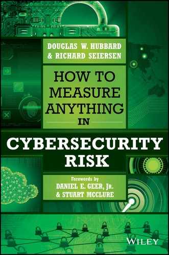
Of course, we know that changes can be due to many factors and a certain amount of volatility is to be expected even if there weren’t a breach. So the way to look at these sorts of events is to consider how big the changes are compared to historical volatility in sales and stock prices. Figure 6.1 shows changes— relative to the time of the breach—for the quarterly sales of three major retailers that had highly publicized data breaches: Home Depot, JCPenney, and Target. Figure 6.2 shows changes in stock prices for those firms and Anthem.
Figures 6.1 and 6.2 don’t appear to show significant changes after a breach compared to the volatility before the breach. To see the detail better, let’s just show changes relative to historical volatility. In Figures 6.3 and 6.4, historical volatility on sales and stock prices is shown as an interval representing the fifth and ninety-fifth percentile of changes for three years up until the breach. The markers show the change after the breach compared to the range of historical volatility (the vertical dashed lines). The changes in sales and the changes in stock prices after the breach are shown relative to their historical volatility.
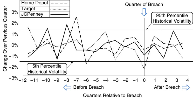
Figure 6.1 Quarter-to-Quarter Change in Sales for Major Retailers with Major Data Breaches Relative to the Quarter of the Breach
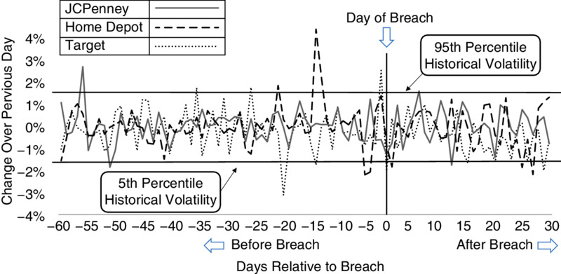
Figure 6.2 Day-to-Day Change in Stock Prices of Firms with Major Data Breaches Relative to Day of the Breach
Figure 6.3 Changes in Stock Prices after a Major Breach for Three Major Retailers Relative to Historical Volatility

Figure 6.4 Changes in Seasonally Adjusted Quarterly Sales after Breach Relative to Historical Volatility
Clearly, any relationship between a major data breach and sales or stock prices—even for breaches as large as Home Depot and Target—is weak at best. While it does look like they might have resulted in some downward movement on average, the movement is explainable as the historical “noise” of day-to-day or quarter-to-quarter changes. In March 2015, another analysis by Trefis published in Forbes magazine indicated that while Home Depot did not actually lose business in the quarters after the breach, management reported other losses in the form of expenses dealing with the event, including “legal help, credit card fraud, and card re-issuance costs going forward.”10
How about the 14% price drop Target experienced in the two-month period after the breach? Well, that too needs to be put in context. Earlier in the same year as the Target breach, we can find another 14% drop in Target’s stock price in the two-month August-to-September period. And by November of 2014 the stock had surpassed the price just before the breach.
What about the survey indicating how customers would abandon retailers hit by a major breach? All we can say is that the sales figures don’t agree with the statements of survey respondents. This is not inconsistent with the fact that what people say on a survey about their value of privacy and security does not appear to model what they actually do, as one Australian study shows.11 Trefis even applied a caveat on the observed decline in sales for Target, saying that “industry-wide foot traffic is already declining due to gradual customer shift to online channel, where Target’s presence is almost negligible.”12 Trefis also said of Home Depot:
In spite of dealing with a case that is bigger than the data breach at Target in late 2013, Home Depot is not expected to lose out on much revenue. Part of this is because the retailer will continue to reap the benefits of an upbeat U.S. economy and housing market. Furthermore, unlike Target, where consumers moved to the likes of Costco or Kohl’s, there are hardly any substitutes when it comes to buying material such as plywood, saws, cement, or the like.13
So apparently there could be other factors regarding whether a retailer sees any impact on customer retention. Perhaps as part of the real “loss of reputation,” it is also a function of where your customers could go for the same products and services. And yet even when these factors apply, as in the case of Target, it is still hard to separate the impact from routine market noise.
Finally, when we look back at past reports about the cost of data breaches, something doesn’t add up. The 2007 data breach at T.J. Maxx was estimated to cost over $1.7 billion.14 Enough time has passed that we should have seen even the delayed impacts realized by now. But if anything approaching that amount were actually experienced, it seems well hidden in their financial reports. The firm was making an annual income from operations of around $700 million or so in the years prior to the breach, which went up to about $1.2 billion at some point after the breach. Annual reports present accounting data at a highly aggregated level, but an impact even half that size should be clearly visible in at least one of those years. Yet we don’t see such an obvious impact in profit, expenses, or even cash or new loans. It certainly did cost T.J. Maxx something but there is no evidence it was anything close to $1.7 billion.
It’s not impossible to lose business as a result of a data breach, but the fact that it is hard to tease out this effect from normal day-to-day or even quarter-to-quarter variations helps inform a practical approach to modeling these losses. Marshall Kuypers, a PhD candidate in management science and engineering at Stanford, has focused his study on these issues. As Kuypers tells the authors:
Academic research has studied the impact of data breach announcements on the stock price of organizations and has consistently found little evidence that the two are related. It is difficult to identify a relationship because signals dissipate quickly and the statistically significant correlation disappears after roughly 3 days.
A Better Way to Model Reputation Damage: Penance Projects
We aren’t saying major data breaches are without costs. There are real costs associated with them, but we need to think about how to model them differently than with vague references to reputation. The actual “reputation” losses may be more realistically modeled as a series of very tangible costs we call “penance projects” as well as other internal and legal liabilities. Penance projects are expenses incurred to limit the long-term impact of loss of reputation. In other words, companies appear to engage in efforts to control damage to reputation instead of bearing what could otherwise be much greater damage. The effect these efforts have on reducing the real loss to reputation seem to be enough that the impact seems hard to detect in sales or stock prices. These efforts include the following:
- Major new investments in cybersecurity systems and policies to correct cybersecurity weaknesses.
- Replacing a lot of upper management responsible for cybersecurity (It may be scapegoating, but it may be necessary for the purpose of addressing reputation.)
- A major public relations push to convince customers and shareholders the problem is being addressed (this helps get the message out that the efforts of the preceding bullet points will solve the problem).
- Marketing and advertising campaigns (separate from getting the word out about how the problem has been confidently addressed) to offset potential losses in business
These damage-control efforts to limit reputation effects appear to be the real costs here—not so much reputation damage itself. Each of these are conveniently concrete measures for which we have multiple historical examples. Of course, if you really do believe that there are other costs to reputation damage, you should model them. But what does reputation damage really mean to a business if you can detect impacts on neither sales nor stock prices? Just be sure you have an empirical basis for your claim. Otherwise, it might be simpler to stick with the penance project cost strategy.
So, if we spend a little more time and effort in analysis, it should be possible to tease out reasonable estimates even for something that seems as “intangible” as reputation loss.
Conclusion
A little decomposition can be very helpful up to a point. To that end, we showed a simple additional decomposition that you can use to build on the example in Chapter 3. We also mentioned a downloadable spreadsheet example and the descriptions of distributions in Appendix A to give you a few tools to help with this decomposition.
We talked about how some decompositions might be uninformative. We need to decompose in a way that leverages your actual knowledge—however limited our knowledge is, there are a few things we do know—and not speculation upon speculation. Test your decompositions with a simulation and compare them to your original estimate before the decomposition. This will show if you learned anything or show if you should actually make your range wider. We tackled a particularly difficult impact to quantify—loss of reputation—and showed how even that has concrete, observable consequences that can be estimated.
So far, we haven’t spent any time on decomposing the likelihood of an event other than to identify likelihoods for two types of events (availability vs. confidentiality and integrity). This is often a bigger source of uncertainty for the analyst and anxiety for management than the impact. Fortunately, that, too, can be decomposed. We will review how to do that later in Part II.
We also need to discuss where these initial estimates of ranges and probabilities can come from. As we discussed in earlier chapters, the same expert who was previously assigning arbitrary scores to a risk matrix can also be taught to assign subjective probabilities in a way that itself has a measurable performance improvement. Then those initial uncertainties can be updated with some very useful mathematical methods even when it seems like data is sparse. These topics will be dealt with in the next two chapters, “Calibrated Assessments” and “Reducing Uncertainty with Bayesian Methods.”