

Logical configuration performance considerations
|
Important: Before reading this chapter, familiarize yourself with the material that is covered in Chapter 3, “Logical configuration concepts and terminology” on page 31.
|
This chapter introduces a step-by-step approach to configuring the IBM Storage System DS8900F depending on workload and performance considerations:
•DS8900F Starter drive choices
•Reviewing the tiered storage concepts and Easy Tier
•Understanding the configuration principles for optimal performance:
– Workload isolation
– Workload resource-sharing
– Workload spreading
•Analyzing workload characteristics to determine isolation or resource-sharing
•Planning allocation of the DS8900F drive and host connection capacity to identified workloads
•Planning spreading volumes and host connections for the identified workloads
•Planning array sites
•Planning RAID arrays and ranks with RAID-level performance considerations
•Planning extent pools with single-tier and multitier extent pool considerations
•Planning address groups, Logical SubSystems (LSSs), volume IDs, and Count Key Data (CKD) Parallel Access Volumes (PAVs)
•Planning I/O port IDs, host attachments, and volume groups
•Logical configuration
4.1 DS8900F Models
The DS8900F family is the most advanced of the DS8000 offerings to date. The DS8900F family consists of the following high-performance Models:
•DS8910F - Flexibility Class (rack-mounted and racked)
•DS8950F - Agility Class
•DS8980F - Analytic Class
4.1.1 DS8910F
DS8910F has the following characteristics:
•Two IBM Power Systems POWER9 MTM 9009-22A
•8 POWER9 cores per CEC
•From 192 GB to 512 GB of System Memory
•From 8 to 64 Host Adapter Ports
•From 16 to 192 Flash drives
•From 12.8 TB to 2,949 TB of capacity (with 15.36 TB Flash Drives)
•860K of Maximum IOps (4K 70/30 R/W mix)
•Maximum of 21 GB/s (Read)/17 GB/s (Write) of Sequential Read - Write
Below we can see the flash drive types supported by DS8900F:

Figure 4-1 Flash Drives supported by DS8900F
For the DS8910F we have the following suggested Starter drive choices: See Table 4-1 on page 61.
Use these options and a storage sizing tool such as StorM:
Table 4-1 DS8910F Starter Drive choices
|
Configuration size
|
Typical Workload
|
Heavy Workload
|
|
< 60 TB
|
1.92 TB drives
|
800 GB drives
|
|
60 to 200 TB
|
1.92 TB drives
|
1.6 TB drives or
800 GB & 1.92 TB drives |
|
200 TB to 500 TB
|
1.6 TB & 7.68 TB drives
|
3.84 TB drives
|
|
500 TB to 1 PB
|
7.68 TB drives or use DS8950F
|
Use DS8950F
|
Observe the following configuration rules:
•For a tiered configuration always configure an equal or greater number of HPFE Enclosure Pairs and drive sets for the upper tier compared to the lower tier.
•For optimal performance configure at least two HPFE Enclosure Pairs spreading drive sets over the enclosure pairs.
•Use the “Typical” workload selection unless there is a heavy sequential write activity either due to host workload or extensive use of FlashCopy combined with significant host write workload.
•The capacity limits are not intended to be exact, so capacity requirements close to the boundary between two sizes could use either option.
•Use a sizing tool such as StorM.
4.1.2 DS8950F
DS8950F has the following characteristics:
•2 × IBM Power Systems POWER9 MTM 9009-42A
•20/40 POWER9 cores per CEC
•From 512 GB to 3,456 GB of System Memory
•From 8 to 128 Host Adapter Ports
•From 16 to 384 Flash drives
•From 12.8 TB to 5,898 TB of capacity (with 15.36 TB Flash Drives)
•2,300K of Maximum IOps (4K 70/30 R/W mix)
•Maximum of 63 GB/s (Read)/ 32 GB/s (Write) of Sequential Read - Write
Table 4-2 shows suggested Starter drive choices for the DS8950F, which can be used along with some storage sizing tool such as StorM.
Table 4-2 DS8950F Starter drive choices
|
Configuration size
|
Typical Workload
|
Heavy Workload
|
|
< 60 TB
|
Use DS8910F
|
800 GB drives
|
|
60 to 200 TB
|
3.84 TB drives or use DS8910F
|
1.6 TB drives
|
|
200 TB to 800 TB
|
1.6 TB & 7.68 TB drives
|
3.84 TB drives
|
|
800 TB to 1.2 PB
|
7.68 TB drives
|
3.2 TB & 15.36 TB drives
|
|
1.2 PB to 4 PB
|
15.36 TB drives
|
Use multiple DS8950F
|
Observe these configuration rules:
•For a tiered configuration always configure an equal or greater number of HPFE Enclosure Pairs and drive sets for the upper tier compared to the lower tier.
•For optimal performance configure two frames and four HPFE Enclosure Pairs and spread HPFE enclosures, Drive sets and Host Adapters across both frames.
•With a single frame, configure at least two HPFE Enclosure Pairs.
•Use the Typical Workload selection unless there is a heavy sequential write activity either due to host workload or extensive use of FlashCopy combined with significant host write workload.
•The capacity limits are not intended to be exact, so capacity requirements close to the boundary between two sizes could use either option.
•Use a sizing tool such as StorM.
4.1.3 DS8980F
DS8980F has the following characteristics:
•2 × IBM Power Systems POWER9 MTM 9009-42A
•44 POWER9 cores per CEC
•4,352 GB of System Memory
•From 8 to 128 Host Adapter Ports
•From 16 to 384 Flash drives
•From 12.8 TB to 5,898 TB of capacity (with 15.36 TB Flash Drives)
•2,300K of Maximum IOps (4K 70/30 R/W mix)
•Maximum of 63 GB/s (Read)/ 32 GB/s (Write) of Sequential Read - Write
The DS8980F will usually be intended for very heavy workloads, and in occasions of bigger consolidation of several older DS8000 into one new DS. As suggested, Starter drive choice, the one for Heavy Workload as shown for the DS8950F in Table 4-2 on page 61, could apply – but again, use a tool like StorM for the final sizing.
4.1.4 Examples using Starter drive choices
Example 1
In the first example shown in Figure 4-2 , we have around 100 TiB of High-Performance Flash drives of 1.6 TB using two HPFEs in the above left picture.
Using the DS8910F Starter drive choices with 100 TB for a typical workload and then the additional custom-placement option (Feature 06060), it is often better to have 1.92 TB drive distributed in 3 HPFEs as it is shown in the above right-hand picture. The slightly higher costs for the additional HPFE are more than offset by the lower price of Flash Tier 2 drives. And especially if the workload profile is heavily sequential, the right-hand alternative would give you even bigger MB/sec throughput, at a lower price.

Figure 4-2 Example 1: Custom placement with around 100 TiB
Example 2
In the second example, Figure 4-3 , we have around 300 TB being distributed between High-Performance Flash drives of 1.6 TB with High-Capacity Flash of 7.68 TB. The left-hand alternative uses only 2 HPFEs together.

Figure 4-3 Example 2: Custom placement with around 300 TB
For workloads which are heavily skewed, and in case of very specific workload profiles, too much load may end up on the one HPFE pair serving the 1.6 TB drives. In that specific example and given workload profile, again using the custom-placement option (FC0606) to order additional HPFEs for the upper tier might give a lot more performance, and could justify the small additional price for the HPFEs.
Using the sizing tool with your specific workload profile will tell if such an alternative option is beneficial for your case.
4.1.5 Easy Tier Overview
Many storage environments support a diversity of needs and use disparate technologies that cause storage sprawl. In a large-scale storage infrastructure, this environment yields a suboptimal storage design that can be improved only with a focus on data access characteristics analysis and management to provide optimum performance.
For Performance Analysis, I/O has always been the most tricky resource to analyze and where there are some rules to follow such as:
•Avoid many I/O operations in the same volume or LUN.
•No I/O is the best I/O. Or in other words: make use of all kinds of cache:
– Memory cache – use of the memory to avoid I/O operations.
– DS8900F cache – this is the reason for bigger DS8000 caches and better microcode caching techniques. A very high cache-hit ratio is always desirable.
•Placement of high important I/Os or heavy workloads in the Flash High-Performance technology and less important I/Os or near to zero workloads into Flash High-Capacity technology.
Before the Easy Tier technology on DS8000, performance analysts tried to make all kinds of I/O studies (called Seek Analysis) in order to understand on how the I/O operations were distributed, and using this information they allocate the datasets, files, databases into the different disk technologies using the performance objectives.
In a certain way this was very frustrating because some time later (weeks, months) the above behavior changed and they would have to change again the placement of the data.
Easy Tier is a DS8900F microcode technique and when enabled allows a permanent I/O analysis where the hot I/O goes automatically to the best technology and the cold I/O goes to less expensive disks.
4.1.6 IBM System Storage Easy Tier
DS8900F is an All-Flash Array (AFA) and it comes with HPFE Gen2 which is an enclosure that can support both High-Performance Flash Drives and High-Capacity Flash Drives.
The enclosures must be installed in pairs. The HPFEs connect to the I/O enclosures over a PCIe fabric, which increases bandwidth and transaction-processing capability.
Flash Drives types and Tiers:
•High-Performance Flash Drives (Tier 0)
– 800 GB
– 1.6 TB
– 3.2 TB
•High-Capacity Flash Drives
– 1.92 TB (Tier 2)
– 3.84 TB (Tier 1)
– 7.68 TB (Tier 2)
– 15.36 TB (Tier 2
With dramatically high I/O rates, low response times, and IOPS-energy-efficient characteristics, flash addresses the highest performance needs and also potentially can achieve significant savings in operational costs. It is critical to choose the correct mix of storage tiers and the correct data placement to achieve optimal storage performance and economics across all tiers at a low cost.
With the DS8900F storage system, you can easily implement tiered storage environments that use high-performance flash and high-capacity flash storage tiers. Still, different storage tiers can be isolated to separate extent pools and volume placement can be managed manually across extent pools where required. Or, better and highly encouraged, volume placement can be managed automatically on a subvolume level (extent level) in hybrid extent pools by Easy Tier automatic mode with minimum management effort for the storage administrator. Easy Tier is a no-cost feature on DS8900F storage systems. For more information about Easy Tier, see 1.2.4, “Easy Tier” on page 11.
Consider Easy Tier automatic mode and hybrid or multi-tier extent pools for managing tiered storage on the DS8900F storage system. The overall management and performance monitoring effort increases considerably when manually managing storage capacity and storage performance needs across multiple storage classes and does not achieve the efficiency provided with Easy Tier automatic mode data relocation on the subvolume level (extent level). With Easy Tier, client configurations show less potential to waste flash capacity than with volume-based tiering methods.
With Easy Tier, you can configure hybrid or multi-tier extent pools (mixed high-performance flash/high-capacity flash storage pools) and turn on Easy Tier on. It then provides automated data relocation across the storage tiers and ranks in the extent pool to optimize storage performance and storage economics. It also rebalances the workload across the ranks within each storage tier (auto-rebalance) based on rank utilization to minimize skew and hot spots. Furthermore, it constantly adapts to changing workload conditions. There is no need anymore to bother with tiering policies that must be manually applied to accommodate changing workload dynamics.
In environments with homogeneous system configurations or isolated storage tiers that are bound to different homogeneous extent pools, you can benefit from Easy Tier automatic mode. Easy Tier provides automatic intra-tier performance management by rebalancing the workload across ranks (auto-rebalance) in homogeneous single-tier pools based on rank utilization. Easy Tier automatically minimizes skew and rank hot spots and helps to reduce the overall management effort for the storage administrator.
Depending on the particular storage requirements in your environment, with the DS8900F architecture, you can address a vast range of storage needs combined with ease of management. On a single DS8900F storage system, you can perform these tasks:
•Isolate workloads to selected extent pools (or down to selected ranks and DAs).
•Share resources of other extent pools with different workloads.
•Use Easy Tier to manage automatically multitier extent pools with different storage tiers (or homogeneous extent pools).
•Adapt your logical configuration easily and dynamically at any time to changing performance or capacity needs by migrating volumes across extent pools, merging extent pools, or removing ranks from one extent pool (rank depopulation) and moving them to another pool.
Easy Tier helps you consolidate more workloads onto a single DS8900F storage system by automating storage performance and storage economics management across up to three drive tiers.
For many initial installations, an approach with two extent pools (with or without different storage tiers) and enabled Easy Tier automatic management might be the simplest way to start if you have FB or CKD storage only; otherwise, four extent pools are required. You can plan for more extent pools based on your specific environment and storage needs, for example, workload isolation for some pools, different resource sharing pools for different departments or clients, or specific Copy Services considerations.
Considerations, as described in 4.2, “Configuration principles for optimal performance” on page 66, apply for planning advanced logical configurations in complex environments, depending on your specific requirements.
4.2 Configuration principles for optimal performance
There are three major principles for achieving a logical configuration on a DS8900F storage system for optimal performance when planning extent pools:
•Workload isolation
•Workload resource-sharing
•Workload spreading
Easy Tier provides a significant benefit for mixed workloads, so consider it for resource-
sharing workloads and isolated workloads dedicated to a specific set of resources. Furthermore, Easy Tier automatically supports the goal of workload spreading by distributing the workload in an optimum way across all the dedicated resources in an extent pool. It provides automated storage performance and storage economics optimization through dynamic data relocation on extent level across multiple storage tiers and ranks based on their access patterns. With auto-rebalance, it rebalances the workload across the ranks within a storage tier based on utilization to reduce skew and avoid hot spots. Auto-rebalance applies to managed multitier pools and single-tier pools and helps to rebalance the workloads evenly across ranks to provide an overall balanced rank utilization within a storage tier or managed single-tier extent pool. Figure 4-4 shows the effect of auto-rebalance in a single-tier extent pool that starts with a highly imbalanced workload across the ranks at T1. Auto-rebalance rebalances the workload and optimizes the rank utilization over time.
sharing workloads and isolated workloads dedicated to a specific set of resources. Furthermore, Easy Tier automatically supports the goal of workload spreading by distributing the workload in an optimum way across all the dedicated resources in an extent pool. It provides automated storage performance and storage economics optimization through dynamic data relocation on extent level across multiple storage tiers and ranks based on their access patterns. With auto-rebalance, it rebalances the workload across the ranks within a storage tier based on utilization to reduce skew and avoid hot spots. Auto-rebalance applies to managed multitier pools and single-tier pools and helps to rebalance the workloads evenly across ranks to provide an overall balanced rank utilization within a storage tier or managed single-tier extent pool. Figure 4-4 shows the effect of auto-rebalance in a single-tier extent pool that starts with a highly imbalanced workload across the ranks at T1. Auto-rebalance rebalances the workload and optimizes the rank utilization over time.

Figure 4-4 Effect of auto-rebalance on individual rank utilization in the system
4.2.1 Workload isolation
With workload isolation, a high-priority workload uses dedicated DS8000 hardware resources to reduce the impact of less important workloads. Workload isolation can also mean limiting a lower-priority workload to a subset of the DS8000 hardware resources so that it does not affect more important workloads by fully using all hardware resources.
Isolation provides ensured availability of the hardware resources that are dedicated to the isolated workload. It removes contention with other applications for those resources.
However, isolation limits the isolated workload to a subset of the total DS8900F hardware so that its maximum potential performance might be reduced. Unless an application has an entire DS8900F storage system that is dedicated to its use, there is potential for contention with other applications for any hardware (such as cache and processor resources) that is not dedicated. Typically, isolation is implemented to improve the performance of certain workloads by separating different workload types.
One traditional practice to isolation is to identify lower-priority workloads with heavy I/O demands and to separate them from all of the more important workloads. You might be able to isolate multiple lower priority workloads with heavy I/O demands to a single set of hardware resources and still meet their lower service-level requirements, particularly if their peak I/O demands are at different times.
|
Important: For convenience, this chapter sometimes describes isolation as a single isolated workload in contrast to multiple resource-sharing workloads, but the approach also applies to multiple isolated workloads.
|
DS8900F flash drive capacity isolation
The level of drive capacity isolation that is required for a workload depends on the scale of its I/O demands as compared to the DS8900F array and DA capabilities, and organizational considerations, such as the importance of the workload and application administrator requests for workload isolation.
You can partition the DS8900F flash drive capacity for isolation at several levels:
•Rank level: Certain ranks are dedicated to a workload, that is, volumes for one workload are allocated on these ranks. The ranks can have a different disk type (capacity or speed), a different RAID array type (RAID 5, RAID 6, or RAID 10, arrays with spares or arrays without spares, RAID 6 being the default), or a different storage type (CKD or FB) than the drive types, RAID array types, or storage types that are used by other workloads. Workloads that require different types of the above can dictate rank, extent pool, and address group isolation. You might consider workloads with heavy random activity for rank isolation, for example.
•Extent pool level: Extent pools are logical constructs that represent a group of ranks that are serviced by storage server 0 or storage server 1. You can isolate different workloads to different extent pools, but you always must be aware of the rank and DA pair (HPFE) associations. Although physical isolation on rank and DA/HPFE level involves building appropriate extent pools with a selected set of ranks or ranks from a specific HPFE/DA pair, different extent pools with a subset of ranks from different DA pairs still can share DAs. Isolated workloads to different extent pools might share a DA adapter as a physical resource, which can be a potential limiting physical resource under certain extreme conditions. However, given the capabilities of one DA or HPFE, some mutual interference there is rare, and isolation (if needed) on extent pool level is effective if the workloads are disk-bound.
•DA (HPFE) level: All ranks on one or more DA pairs or a HPFE pair are dedicated to a workload, that is, only volumes for this workload are allocated on the ranks that are associated with one or more DAs. These ranks can be a different disk type (capacity or speed), RAID array type (RAID 5, RAID 6, or RAID 10, arrays with spares or arrays without spares), or storage type (CKD or FB) than the disk types, RAID types, or storage types that are used by other workloads. Consider only huge (multiple GBps) workloads with heavy, large blocksize, and sequential activity for DA-level/HPFE-level isolation because these workloads tend to consume all of the available DA resources.
•Processor complex level: All ranks that are assigned to extent pools managed by processor complex 0 or all ranks that are assigned to extent pools managed by processor complex 1 are dedicated to a workload. This approach is not preferable because it can reduce the processor and cache resources and the back-end bandwidth that is available to the workload by 50%.
•Storage unit level: All ranks in a physical DS8900F storage system are dedicated to a workload, that is, the physical DS8900F storage system runs one workload.
•Pinning volumes to a tier in hybrid pools: This level is not complete isolation, but it can be a preferred way to go in many cases. Even if you have just one pool pair with two large three-tier pools, you may use the High-Performance flash tier only for some volumes and the High-Capacity flash tier only for others. Certain volumes may float only among ranks of the upper tier or between the upper tiers only, but lower tiers are excluded for them, and the other way round for other volumes. Such a setup allows a simple extent pool structure, and at the same time less-prioritized volumes stay on lower tiers only and highly prioritized volumes are treated preferentially. The way you do such pinning could also be changed at any time.
DS8000 host connection isolation
The level of host connection isolation that is required for a workload depends on the scale of its I/O demands as compared to the DS8900F I/O port and host adapter (HA) capabilities. It also depends on organizational considerations, such as the importance of the workload and administrator requests for workload isolation.
The DS8900F host connection subsetting for isolation can also be done at several levels:
•I/O port level: Certain DS8900F I/O ports are dedicated to a workload, which is a common case. Workloads that require Fibre Channel connection (FICON) and Fibre Channel Protocol (FCP) must be isolated at the I/O port level anyway because each I/O port on a FCP/FICON-capable HA card can be configured to support only one of these protocols. Although Open Systems host servers and remote mirroring links use the same protocol (FCP), they are typically isolated to different I/O ports. You must also consider workloads with heavy large-block sequential activity for HA isolation because they tend to consume all of the I/O port resources that are available to them.
•HA level: Certain HAs are dedicated to a workload. FICON and FCP workloads do not necessarily require HA isolation because separate I/O ports on the same FCP/FICON-
capable HA card can be configured to support each protocol (FICON or FCP). However, it is a preferred practice to separate FCP and FICON to different HBAs. Furthermore, host connection requirements might dictate a unique type of HA card (longwave (LW) or shortwave (SW)) for a workload. Workloads with heavy large-block sequential activity must be considered for HA isolation because they tend to consume all of the I/O port resources that are available to them.
capable HA card can be configured to support each protocol (FICON or FCP). However, it is a preferred practice to separate FCP and FICON to different HBAs. Furthermore, host connection requirements might dictate a unique type of HA card (longwave (LW) or shortwave (SW)) for a workload. Workloads with heavy large-block sequential activity must be considered for HA isolation because they tend to consume all of the I/O port resources that are available to them.
•I/O enclosure level: Certain I/O enclosures are dedicated to a workload. This approach is not necessary.
4.2.2 Workload resource-sharing
Workload resource-sharing means multiple workloads use a common set of the DS8900F hardware resources:
•Ranks
•DAs and HPFEs
•I/O ports
•HAs
Multiple resource-sharing workloads can have logical volumes on the same ranks and can access the same DS8900F HAs or I/O ports. Resource-sharing allows a workload to access more DS8900F hardware than can be dedicated to the workload, providing greater potential performance, but this hardware sharing can result in resource contention between applications that impacts overall performance at times. It is important to allow resource-sharing only for workloads that do not consume all of the DS8900F hardware resources that are available to them. Pinning volumes to one certain tier can also be considered temporarily, and then you can release these volumes again.
Easy Tier extent pools typically are shared by multiple workloads because Easy Tier with its automatic data relocation and performance optimization across multiple storage tiers provides the most benefit for mixed workloads.
To better understand the resource-sharing principle for workloads on disk arrays, see 3.2.3, “Extent pool considerations” on page 51.
4.2.3 Workload spreading
Workload spreading means balancing and distributing overall workload evenly across all of the DS8900F hardware resources that are available:
•Processor complex 0 and processor complex 1
•HPFEs and DAs
•Ranks
•I/O enclosures
•HAs
Spreading applies to both isolated workloads and resource-sharing workloads.
You must allocate the DS8900F hardware resources to either an isolated workload or multiple resource-sharing workloads in a balanced manner, that is, you must allocate either an isolated workload or resource-sharing workloads to the DS8900F ranks that are assigned to DAs and both processor complexes in a balanced manner. You must allocate either type of workload to I/O ports that are spread across HAs and I/O enclosures in a balanced manner.
You must distribute volumes and host connections for either an isolated workload or a resource-sharing workload in a balanced manner across all DS8900F hardware resources that are allocated to that workload.
You should create volumes as evenly distributed as possible across all ranks and DAs allocated to those workloads.
One exception to the recommendation of spreading volumes might be when specific files or data sets are never accessed simultaneously, such as multiple log files for the same application where only one log file is in use at a time. In that case, you can place the volumes required by these data sets or files on the same resources.
You must also configure host connections as evenly distributed as possible across the I/O ports, HAs, and I/O enclosures that are available to either an isolated or a resource-sharing workload. Then, you can use host server multipathing software to optimize performance over multiple host connections. For more information about multipathing software, see Chapter 8, “Host attachment” on page 187.
4.2.4 Using workload isolation, resource-sharing, and spreading
When you perform DS8900F performance optimization, you must first identify any workload that has the potential to negatively impact the performance of other workloads by fully using all of the DS8900F I/O ports and the DS8900F ranks available to it.
Additionally, you might identify any workload that is so critical that its performance can never be allowed to be negatively impacted by other workloads.
Then, identify the remaining workloads that are considered appropriate for resource-sharing.
Next, define a balanced set of hardware resources that can be dedicated to any isolated workloads, if required. Then, allocate the remaining DS8000 hardware for sharing among the resource-sharing workloads. Carefully consider the appropriate resources and storage tiers for Easy Tier and multitier extent pools in a balanced manner.
The next step is planning extent pools and assigning volumes and host connections to all workloads in a way that is balanced and spread. By default, the standard allocation method when creating volumes is stripes with one-extent granularity across all arrays in a pool, so on the rank level, this distribution is done automatically.
Without the explicit need for workload isolation or any other requirements for multiple extent pools, starting with two extent pools (with or without different storage tiers) and a balanced distribution of the ranks and DAs/HPFEs might be the simplest configuration to start with using resource-sharing throughout the whole DS8900F storage system and Easy Tier automatic management if you have either FB or CKD storage. Otherwise, four extent pools are required for a reasonable minimum configuration, two for FB storage and two for CKD storage, and each pair is distributed across both DS8900F storage servers.
The final step is the implementation of host-level striping (when appropriate) and multipathing software, if needed. If you planned for Easy Tier, do not consider host-level striping because it dilutes the workload skew and is counterproductive to the Easy Tier optimization.
4.3 Analyzing application workload characteristics
The first and most important step in creating a successful logical configuration for the DS8900F storage system is analyzing the workload characteristics for the applications that access the DS8900F storage system. The DS8900F hardware resources, such as RAID arrays and I/O ports, must be correctly allocated to workloads for isolation and resource-sharing considerations. If planning for shared multitier configurations and Easy Tier, it is important to determine the skew of the workload and plan for the amount of required storage capacity on the appropriate storage tiers. You must perform this workload analysis during the DS8900F capacity planning process, and you must complete it before ordering the DS8000 hardware.
4.3.1 Determining skew and storage requirements for Easy Tier
For Easy Tier configurations, it is important to determine the skew of the workload and plan for the amount of required storage capacity on each of the storage tiers. Plan the optimum initial hardware configuration for managed multitier environments so that you determine the overall distribution of the I/O workload against the amount of data (data heat distribution) to understand how much of the data is doing how much (or most) of the I/O workload. The workload pattern, small block random or large block sequential read/write operations, also is important. A good understanding of the workload heat distribution and skew helps to evaluate the benefit of an Easy Tier configuration.
For example, the ratio of High-Performance flash capacity to High-Capacity flash capacity in a hybrid pool depends on the workload characteristics and skew.
For a two-tier configuration always configure an equal or greater number of HPFE Enclosure Pairs and drive sets for the upper tier compared to the lower tier. You should not use less drives of High-Performance flash (Tier 0) than of High-Capacity flash (Tier 2). For instance, mixing High-Performance flash of 3.2 TB with High-Capacity flash of 15.36 TB under these conditions, you already come to almost 20% of net capacity in Flash Tier 0.
The DS8900F Storage Management GUI also can provide guidance for capacity planning of the available storage tiers based on the existing workloads on a DS8900F storage system with Easy Tier monitoring enabled.
4.3.2 Determining isolation requirements
The objective of this analysis is to identify workloads that require isolated (dedicated) DS8900F hardware resources because this determination ultimately affects the total amount of disk capacity that is required and the total number of disk drive types that is required, and the number and type of HAs that is required. The result of this first analysis indicates which workloads require isolation and the level of isolation that is required.
You must also consider organizational and business considerations in determining which workloads to isolate. Workload priority (the importance of a workload to the business) is a key consideration. Application administrators typically request dedicated resources for high priority workloads. For example, certain database online transaction processing (OLTP) workloads might require dedicated resources to ensure service levels.
The most important consideration is preventing lower-priority workloads with heavy I/O requirements from impacting higher priority workloads. Lower-priority workloads with heavy random activity must be evaluated for rank isolation. Lower-priority workloads with heavy, large blocksize, and sequential activity must be evaluated for I/O port, and eventually DA (HPFE) isolation.
Workloads that require different disk drive types (capacity and speed), different RAID types (RAID 5, RAID 6, or RAID 10), or different storage types (CKD or FB) dictate isolation to different DS8000 arrays, ranks, and extent pools, unless this situation can be solved by pinning volumes to one certain tier. For more information about the performance implications of various RAID types, see “RAID-level performance considerations” on page 77.
Workloads that use different I/O protocols (FCP or FICON) dictate isolation to different I/O ports. However, workloads that use the same drive types, RAID type, storage type, and I/O protocol can be evaluated for separation or isolation requirements.
Workloads with heavy, continuous I/O access patterns must be considered for isolation to prevent them from consuming all available DS8900F hardware resources and impacting the performance of other types of workloads. Workloads with large blocksize and sequential activity can be considered for separation from those workloads with small blocksize and random activity.
Isolation of only a few workloads that are known to have high I/O demands can allow all the remaining workloads (including the high-priority workloads) to share hardware resources and achieve acceptable levels of performance. More than one workload with high I/O demands might be able to share the isolated DS8900F resources, depending on the service level requirements and the times of peak activity.
The following examples are I/O workloads, files, or data sets that might have heavy and continuous I/O access patterns:
•Sequential workloads (especially those workloads with large-blocksize transfers)
•Log files or data sets
•Sort or work data sets or files
•Business Intelligence and Data Mining
•Disk copies (including Point-in-Time Copy background copies, remote mirroring target volumes, and tape simulation on disk)
•Video and imaging applications
•Engineering and scientific applications
•Certain batch workloads
You must consider workloads for all applications for which DS8900F storage is allocated, including current workloads to be migrated from other installed storage systems and new workloads that are planned for the DS8900F storage system. Also, consider projected growth for both current and new workloads.
For existing applications, consider historical experience first. For example, is there an application where certain data sets or files are known to have heavy, continuous I/O access patterns? Is there a combination of multiple workloads that might result in unacceptable performance if their peak I/O times occur simultaneously? Consider workload importance (workloads of critical importance and workloads of lesser importance).
For existing applications, you can also use performance monitoring tools that are available for the existing storage systems and server platforms to understand current application workload characteristics:
•Read/write ratio
•Random/sequential ratio
•Average transfer size (blocksize)
•Peak workload (IOPS for random access and MB per second for sequential access)
•Peak workload periods (time of day and time of month)
•Copy Services requirements (Point-in-Time Copy and Remote Mirroring)
•Host connection utilization and throughput (FCP host connections and FICON)
•Remote mirroring link utilization and throughput
Estimate the requirements for new application workloads and for current application workload growth. You can obtain information about general workload characteristics in Chapter 5, “Understanding your workload” on page 107.
As new applications are rolled out and current applications grow, you must monitor performance and adjust projections and allocations. You can obtain more information about this topic in Chapter 7, “Practical performance management” on page 139.
You can use the StorM modeling tool to model the current or projected workload and estimate the required DS8900F hardware resources. They are described in Chapter 6, “Performance planning tools” on page 125.
The DS8900F Storage Management GUI can also provide workload information and capacity planning recommendations that are associated with a specific workload to reconsider the need for isolation and evaluate the potential benefit when using a multitier configuration and Easy Tier.
4.3.3 Reviewing remaining workloads for feasibility of resource-sharing
After workloads with the highest priority or the highest I/O demands are identified for isolation, the I/O characteristics of the remaining workloads must be reviewed to determine whether a single group of resource-sharing workloads is appropriate, or whether it makes sense to split the remaining applications into multiple resource-sharing groups. The result of this step is the addition of one or more groups of resource-sharing workloads to the DS8900F configuration plan.
4.4 Planning allocation of disk and host connection capacity
You must plan the allocation of specific DS8900F hardware first for any isolated workload, and then for the resource-sharing workloads, including Easy Tier hybrid pools. Use the workload analysis in 4.3.2, “Determining isolation requirements” on page 71 to define the flash capacity and host connection capacity that is required for the workloads. For any workload, the required flash capacity is determined by both the amount of space that is needed for data and the number of arrays (of a specific speed) that are needed to provide the needed level of performance. The result of this step is a plan that indicates the number of ranks (including disk drive type) and associated DAs and the number of I/O adapters and associated I/O enclosures that are required for any isolated workload and for any group of resource-sharing workloads.
Planning DS8000 hardware resources for isolated workloads
For the DS8900F flash allocation, isolation requirements might dictate the allocation of certain individual ranks or all of the ranks on certain DAs to one workload. For the DS8900F I/O port allocation, isolation requirements might dictate the allocation of certain I/O ports or all of the I/O ports on certain HAs to one workload.
Choose the DS8900F resources to dedicate in a balanced manner. If ranks are planned for workloads in multiples of two, half of the ranks can later be assigned to extent pools managed by processor complex 0, and the other ranks can be assigned to extent pools managed by processor complex 1. You may also note the DAs and HPFEs to be used. If I/O ports are allocated in multiples of four, they can later be spread evenly across all I/O enclosures in a DS8900F frame if four or more HA cards are installed. If I/O ports are allocated in multiples of two, they can later be spread evenly across left and right I/O enclosures.
Planning DS8900F hardware resources for resource-sharing workloads
Review the DS8900F resources to share for balance. If ranks are planned for resource-sharing workloads in multiples of two, half of the ranks can later be assigned to processor complex 0 extent pools, and the other ranks can be assigned to processor complex 1 extent pools. If I/O ports are allocated for resource-sharing workloads in multiples of four, they can later be spread evenly across all I/O enclosures in a DS8900F frame if four or more HA cards are installed. If I/O ports are allocated in multiples of two, they can later be spread evenly across left and right I/O enclosures.
Easy Tier later provides automatic intra-tier management in single-tier and multitier pools (auto-rebalance) and cross-tier management in multitier pools for the resource-sharing workloads.
4.5 Planning volume and host connection spreading
After hardware resources are allocated for both isolated and resource-sharing workloads, plan the volume and host connection spreading for all of the workloads.
|
Host connection: In this chapter, we use host connection in a general sense to represent a connection between a host server (either z Operating Systems or Open Systems) and the DS8000 storage system.
|
The result of this step is a plan that includes this information:
•The specific number and size of volumes for each isolated workload or group of resource-sharing workloads and how they are allocated to ranks and DAs
•The specific number of I/O ports for each workload or group of resource-sharing workloads and how they are allocated to HAs and I/O enclosures
After the spreading plan is complete, use the DS8900F hardware resources that are identified in the plan as input to order the DS8900F hardware.
4.5.1 Spreading volumes for isolated and resource-sharing workloads
Now, consider the requirements of each workload for the number and size of logical volumes. For a specific amount of required disk capacity from the perspective of the DS8900F storage system, there are typically no significant DS8900F performance implications of using more small volumes as compared to fewer large volumes. However, using one or a few standard volume sizes can simplify management.
However, there are host server performance considerations related to the number and size of volumes. For example, for z Systems servers, the number of PAVs that are needed can vary with volume size. For more information about PAVs, see 10.2, “DS8000 and z Systems planning and configuration” on page 245.
There also can be Open Systems host server or multipathing software considerations that are related to the number or the size of volumes, so you must consider these factors in addition to workload requirements.
There are significant performance implications with the assignment of logical volumes to ranks and DAs. The goal of the entire logical configuration planning process is to ensure that volumes for each workload are on ranks and DAs that allow all workloads to meet performance objectives.
To spread volumes across allocated hardware for each isolated workload, and then for each workload in a group of resource-sharing workloads, complete the following steps:
1. Review the required number and the size of the logical volumes that are identified during the workload analysis.
2. Review the number of ranks that are allocated to the workload (or group of resource-sharing workloads) and the associated DA pairs.
3. Evaluate the use of multi-rank or multitier extent pools. Evaluate the use of Easy Tier in automatic mode to automatically manage data placement and performance.
4. Assign the volumes, preferably with the default allocation method rotate extents (DSCLI term: rotateexts, GUI: rotate capacity).
4.5.2 Spreading host connections for isolated and resource-sharing workloads
Next, consider the requirements of each workload for the number and type of host connections. In addition to workload requirements, you also might need to consider the host server or multipathing software in relation to the number of host connections. For more information about multipathing software, see Chapter 8, “Host attachment” on page 187.
There are significant performance implications from the assignment of host connections to I/O ports, HAs, and I/O enclosures. The goal of the entire logical configuration planning process is to ensure that host connections for each workload access I/O ports and HAs that allow all workloads to meet the performance objectives.
To spread host connections across allocated hardware for each isolated workload, and then for each workload in a group of resource-sharing workloads, complete the following steps:
1. Review the required number and type (SW, LW, FCP, or FICON) of host connections that are identified in the workload analysis. You must use a minimum of two host connections to different DS8900F HA cards to ensure availability. Some Open Systems hosts might impose limits on the number of paths and volumes. In such cases, you might consider not exceeding four paths per volume, which in general is a good approach for performance and availability. The DS8900F front-end host ports are 16 Gbps and 32 Gbps capable and if the expected workload is not explicitly saturating the adapter and port bandwidth with high sequential loads, you might share ports with many hosts.
2. Review the HAs that are allocated to the workload (or group of resource-sharing workloads) and the associated I/O enclosures.
3. Review requirements that need I/O port isolation, for example, remote replication Copy Services, or SAN Volume Controller. If possible, try to split them as you split hosts among hardware resources. Do not mix them with other Open Systems because they can have different workload characteristics.
4. Assign each required host connection to a different HA in a different I/O enclosure if possible, balancing them across the left and right I/O enclosures:
– If the required number of host connections is less or equal than the available number of I/O enclosures (which can be typical for certain Open Systems servers), assign an equal number of host connections to left I/O enclosures (0, 2, 4, and 6) as to right I/O enclosures (1, 3, 5, and 7).
– Within an I/O enclosure, assign each required host connection to the HA of the required type (SW FCP/FICON-capable or LW FCP/FICON-capable) with the greatest number of unused ports. When HAs have an equal number of unused ports, assign the host connection to the adapter that has the fewest connections for this workload.
– If the number of required host connections is greater than the number of I/O enclosures, assign the additional connections to different HAs with the most unused ports within the I/O enclosures. When HAs have an equal number of unused ports, assign the host connection to the adapter that has the fewest connections for this workload.
4.6 Planning array sites
During the DS8900F installation, array sites are dynamically created and assigned to HPFEs and their DA pairs. Array site IDs (Sx) do not have any fixed or predetermined relationship to drive physical locations or to the flash enclosure installation order. The relationship between array site IDs and physical drive locations or DA assignments can differ between the DS8900F storage systems, even on the DS8900F storage systems with the same number and type of flash drives.
When using the DS Storage Manager GUI to create managed arrays and pools, the GUI automatically chooses a good distribution of the arrays across all DAs, and initial formatting with the GUI gives optimal results for many cases. Only for specific requirements (for example, isolation by DA pairs) is the command-line interface (DSCLI) advantageous because it gives more options for a certain specific configuration.
After the DS8900F hardware is installed, you can use the output of the DS8000 DSCLI lsarraysite command to display and document array site information, including flash drive type and DA pair. Check the disk drive type and DA pair for each array site to ensure that arrays, ranks, and ultimately volumes that are created from the array site are created on the DS8900F hardware resources required for the isolated or resource-sharing workloads.
The result of this step is the addition of specific array site IDs to the plan of workload assignment to ranks.
4.7 Planning RAID arrays and ranks
The next step is planning the RAID arrays and ranks. When using DSCLI, take the specific array sites that are planned for isolated or resource-sharing workloads and define their assignments to RAID arrays and CKD or FB ranks, and thus define array IDs and rank IDs. Because there is a one-to-one correspondence between an array and a rank on the DS8900F storage system, you can plan arrays and ranks in a single step. However, array creation and rank creation require separate steps.
The sequence of steps when creating the arrays and ranks with the DSCLI finally determines the numbering scheme of array IDs and rank IDs because these IDs are chosen automatically by the system during creation. The logical configuration does not depend on a specific ID numbering scheme, but a specific ID numbering scheme might help you plan the configuration and manage performance more easily.
|
Storage servers: Array sites, arrays, and ranks do not have a fixed or predetermined relationship to any DS8900F processor complex (storage server) before they are finally assigned to an extent pool and a rank group (rank group 0/1 is managed by processor complex 0/1).
|
RAID-level performance considerations
The available drive options provide industry-class capacity and performance to address a wide range of business requirements. The DS8900F storage arrays can be configured as RAID 6, RAID 10, or RAID 5, depending on the drive type.
RAID 6 is now the default and preferred setting for the DS8900F. RAID 5 can be configured for drives of less than 1 TB, but this configuration is not preferred and requires a risk acceptance. Flash Tier 0 drive sizes larger than 1 TB can be configured by using RAID 5, but require an RPQ and an internal control switch to be enabled. RAID 10 continues to be an option for all drive types.
When configuring arrays from array sites, you must specify the RAID level, either RAID 5, RAID 6, or RAID 10. These RAID levels meet different requirements for performance, usable storage capacity, and data protection. However, you must determine the correct RAID types and the physical flash drives (speed and capacity) that are related to initial workload performance objectives, capacity requirements, and availability considerations before you order the DS8900F hardware.
Each HPFE Gen2 pair can contain up to six array sites. The first set of 16 flash drives creates two 8-flash drive array sites. RAID 6 arrays are created by default on each array site.
During logical configuration, RAID 6 arrays and the required number of spares are created. Each HPFE Gen2 pair has two global spares, created from the first increment of 16 flash drives. The first two arrays to be created from these array sites are 5+P+Q. Subsequent RAID 6 arrays in the same HPFE Gen2 Pair will be 6+P+Q.
RAID 5 had been for long one of the most commonly used levels of RAID protection because it optimizes cost-effective performance while emphasizing usable capacity through data striping. It provides fault tolerance if one disk drive fails by using XOR parity for redundancy. Hot spots within an array are avoided by distributing data and parity information across all of the drives in the array. The capacity of one drive in the RAID array is lost because it holds the parity information. RAID 5 provides a good balance of performance and usable storage capacity.
RAID 6 provides a higher level of fault tolerance than RAID 5 in disk failures, but also provides less usable capacity than RAID 5 because the capacity of two drives in the array is set aside to hold the parity information. As with RAID 5, hot spots within an array are avoided by distributing data and parity information across all of the drives in the array. Still, RAID 6 offers more usable capacity than RAID 10 by providing an efficient method of data protection in double disk errors, such as two drive failures, two coincident medium errors, or a drive failure and a medium error during a rebuild. Because the likelihood of media errors increases with the capacity of the physical disk drives, consider the use of RAID 6 with large capacity disk drives and higher data availability requirements. For example, consider RAID 6 where rebuilding the array in a drive failure takes a long time.
RAID 6 arrays are created by default on each array site.
RAID 10 optimizes high performance while maintaining fault tolerance for disk drive failures. The data is striped across several disks, and the first set of disk drives is mirrored to an identical set. RAID 10 can tolerate at least one, and in most cases, multiple disk failures if the primary copy and the secondary copy of a mirrored disk pair do not fail at the same time.
Regarding random-write I/O operations, the different RAID levels vary considerably in their performance characteristics. With RAID 10, each write operation at the disk back end initiates two disk operations to the rank. With RAID 5, an individual random small-block write operation to the disk back end typically causes a RAID 5 write penalty, which initiates four I/O operations to the rank by reading the old data and the old parity block before finally writing the new data and the new parity block. For RAID 6 with two parity blocks, the write penalty increases to six required I/O operations at the back end for a single random small-block write operation. This assumption is a worst-case scenario that is helpful for understanding the back-end impact of random workloads with a certain read/write ratio for the various RAID levels. It permits a rough estimate of the expected back-end I/O workload and helps you to plan for the correct number of arrays. On a heavily loaded system, it might take fewer I/O operations than expected on average for RAID 5 and RAID 6 arrays. The optimization of the queue of write I/Os waiting in cache for the next destage operation can lead to a high number of partial or full stripe writes to the arrays with fewer required back-end disk operations for the parity calculation.
On modern disk systems, such as the DS8900F storage system, write operations are cached by the storage subsystem and thus handled asynchronously with short write response times for the attached host systems. So, any RAID 5 or RAID 6 write penalties are shielded from the attached host systems in disk response time. Typically, a write request that is sent to the DS8900F subsystem is written into storage server cache and persistent cache, and the I/O operation is then acknowledged immediately to the host system as complete. If there is free space in these cache areas, the response time that is seen by the application is only the time to get data into the cache, and it does not matter whether RAID 5, RAID 6, or RAID 10 is used.
There is also the concept of rewrites. If you update a cache segment that is still in write cache and not yet destaged, update segment in the cache and eliminate the RAID penalty for the previous write step. However, if the host systems send data to the cache areas faster than the storage server can destage the data to the arrays (that is, move it from cache to the physical disks), the cache can occasionally fill up with no space for the next write request. Therefore, the storage server signals the host system to retry the I/O write operation. In the time that it takes the host system to retry the I/O write operation, the storage server likely can destage part of the data, which provides free space in the cache and allows the I/O operation to complete on the retry attempt.
RAID 10 is not as commonly used as RAID 5 or RAID 6 for the following reason: RAID 10 requires more raw disk capacity for every TB of effective capacity.
Table 4-3 shows a short overview of the advantages and disadvantages for the RAID level reliability, space efficiency, and random write performance.
Table 4-3 RAID-level comparison of reliability, space efficiency, and write penalty
|
RAID level
|
Reliability
(number of erasures)
|
Space efficiency1
|
Performance
write penalty
(number of disk operations)
|
|
RAID 5 (7+P)
|
1
|
87.5%
|
4
|
|
RAID 6 (6+P+Q)
|
2
|
75%
|
6
|
|
RAID 10 (4x2)
|
At least 1
|
50%
|
2
|
1 The space efficiency in this table is based on the number of disks that remain available for data storage. The actual usable decimal capacities are up to 5% less.
Because RAID 5, RAID 6, and RAID 10 perform equally well for both random and sequential read operations, RAID 5 or RAID 6 might be a good choice for space efficiency and performance for standard workloads with many read requests. RAID 6 offers a higher level of data protection than RAID 5, especially for large capacity drives.
For array rebuilds, RAID 5, RAID 6, and RAID 10 require approximately the same elapsed time, although RAID 5 and RAID 6 require more disk operations and therefore are more likely to affect other disk activity on the same disk array.
Today, High-Capacity flash drives are mostly used as some Tier 1 (High-Capacity flash of 3.84 TB) and lower tiers in a hybrid pool where most of the IOPS are handled by Tier 0 High-Performance flash drives. Yet, even if the High-Performance flash tier might handle, for example, 70% and more of the load, the High-Capacity flash drives still handle a considerable workload amount because of their large bulk capacity.
Finally, using the lsarray -l, and lsrank -l commands can give you an idea of which DA pair (HPFE) is used by each array and rank respectively, as shown in Example 4-1. You can do further planning from here.
Example 4-1 lsarray -l and lsrank -l commands showing Array ID sequence and DA pair
dscli> lsarray -l
Array State Data RAIDtype arsite Rank DA Pair DDMcap (10^9B) diskclass encrypt
=========================================================================================
A0 Assigned Normal 6 (6+P+Q) S6 R0 11 1600.0 FlashTier0 supported
A1 Assigned Normal 6 (5+P+Q+S) S2 R1 10 7680.0 FlashTier2 supported
A2 Assigned Normal 6 (6+P+Q) S5 R2 11 1600.0 FlashTier0 supported
A3 Assigned Normal 6 (5+P+Q+S) S1 R3 10 7680.0 FlashTier2 supported
A4 Assigned Normal 6 (5+P+Q+S) S3 R4 11 1600.0 FlashTier0 supported
A5 Assigned Normal 6 (5+P+Q+S) S4 R5 11 1600.0 FlashTier0 supported
dscli> lsrank -l
ID Group State datastate Array RAIDtype extpoolID extpoolnam stgtype exts usedexts keygrp marray extsi
===========================================================================================================
R0 0 Normal Normal A0 6 P0 Open_ET fb 554647 547943 1 MA6 16MiB
R1 0 Normal Normal A1 6 P0 Open_ET fb 2219583 276917 1 MA2 16MiB
R2 1 Normal Normal A2 6 P1 Open_ET fb 554647 553725 1 MA5 16MiB
R3 1 Normal Normal A3 6 P1 Open_ET fb 2219583 1840518 1 MA1 16MiB
R4 0 Normal Normal A4 6 P2 CKD_z/OS ckd 429258 35783 1 MA3 21cyl
R5 1 Normal Normal A5 6 P3 CKD_z/OS ckd 429258 39931 1 MA4 21cyl
4.8 Planning extent pools
After planning the arrays and the ranks, the next step is to plan the extent pools, which means taking the planned ranks and defining their assignment to extent pools and rank groups, including planning the extent pool IDs.
Extent pools are automatically numbered with system-generated IDs starting with P0, P1, and P2 in the sequence in which they are created. Extent pools that are created for rank group 0 are managed by processor complex 0 and have even-numbered IDs (P0, P2, and P4, for example). Extent pools that are created for rank group 1 are managed by processor complex 1 and have odd-numbered IDs (P1, P3, and P5, for example). Only in a failure condition or during a concurrent code load is the ownership of a certain rank group temporarily moved to the alternative processor complex.
To achieve a uniform storage system I/O performance and avoid single resources that become bottlenecks (called hot spots), it is preferable to distribute volumes and workloads evenly across all of the ranks and DA pairs that are dedicated to a workload by creating appropriate extent pool configurations.
The assignment of the ranks to extent pools together with an appropriate concept for the logical configuration and volume layout is the most essential step to optimize overall storage system performance. A rank can be assigned to any extent pool or rank group. Each rank provides a particular number of storage extents of a certain storage type (either FB or CKD) to an extent pool. Finally, an extent pool aggregates the extents from the assigned ranks and provides the logical storage capacity for the creation of logical volumes for the attached host systems.
On the DS8900F storage system, you can configure homogeneous single-tier extent pools with ranks of the same storage class, and hybrid multitier extent pools with ranks from different storage classes. The Extent Allocation Methods (EAM), such as rotate extents or storage-pool striping, provide easy-to-use capacity-based methods of spreading the workload data across the ranks in an extent pool. Furthermore, the use of Easy Tier automatic mode to automatically manage and maintain an optimal workload distribution across these resources over time provides excellent workload spreading with the best performance at a minimum administrative effort.
The following sections present concepts for the configuration of single-tier and multitier extent pools to spread the workloads evenly across the available hardware resources. Also, the benefits of Easy Tier with different extent pool configurations are outlined. Unless otherwise noted, assume that enabling Easy Tier automatic mode refers to enabling the automatic management capabilities of Easy Tier and Easy Tier monitoring.
4.8.1 Single-tier extent pools
Single-tier or homogeneous extent pools are pools that contain ranks from only one storage class or storage tier:
• HPFE High-Performance Flash
• HPFE High-Capacity Flash
Single-tier extent pools consist of one or more ranks that can be referred to as single-rank or multi-rank extent pools.
Single-rank extent pools
With single-rank extent pools, there is a direct relationship between volumes and ranks based on the extent pool of the volume. This relationship helps you manage and analyze performance down to rank level more easily, especially with host-based tools, such as IBM Resource Measurement Facility (IBM RMF) on z Systems in combination with a hardware-related assignment of LSS/LCU IDs. However, the administrative effort increases considerably because you must create the volumes for a specific workload in multiple steps from each extent pool separately when distributing the workload across multiple ranks.
With single-rank extent pools, you choose a configuration design that limits the capabilities of a created volume to the capabilities of a single rank for capacity and performance. A single volume cannot exceed the capacity or the I/O performance provided by a single rank. So, for demanding workloads, you must create multiple volumes from enough ranks from different extent pools and use host-level-based striping techniques, such as volume manager striping, to spread the workload evenly across the ranks dedicated to a specific workload. You are also likely to waste storage capacity easily if extents remain left on ranks in different extent pools because a single volume can be created only from extents within a single extent pool, not across extent pools.
Furthermore, you benefit less from the advanced DS8000 virtualization features, such as dynamic volume expansion (DVE), storage pool striping, Easy Tier automatic performance management, and workload spreading, which use the capabilities of multiple ranks within a single extent pool.
Single-rank extent pools are selected for environments where isolation or management of volumes on the rank level is needed, such as in some z/OS environments. Single-rank extent pools are selected for configurations by using storage appliances, such as the SAN Volume Controller, where the selected RAID arrays are provided to the appliance as simple back-end storage capacity and where the advanced virtualization features on the DS8000 storage system are not required or not wanted to avoid multiple layers of data striping. However, the use of homogeneous multi-rank extent pools and storage pool striping to minimize the storage administrative effort by shifting the performance management from the rank to the extent pool level and letting the DS8000 storage system maintain a balanced data distribution across the ranks within a specific pool is popular. It provides excellent performance in relation to the reduced management effort.
Also, you do not need to strictly use only single-rank extent pools or only multi-rank extent pools on a storage system. You can base your decision on individual considerations for each workload group that is assigned to a set of ranks and thus extent pools. The decision to use single-rank and multi-rank extent pools depends on the logical configuration concept that is chosen for the distribution of the identified workloads or workload groups for isolation and resource-sharing.
In general, single-rank extent pools might not be good in the current complex and mixed environments unless you know that this level of isolation and micro-performance management is required for your specific environment. If not managed correctly, workload skew and rank hot spots that limit overall system performance are likely to occur.
Multi-rank homogeneous extent pools (with only one storage tier)
If the logical configuration concept aims to balance certain workloads or workload groups (especially large resource-sharing workload groups) across multiple ranks with the allocation of volumes or extents on successive ranks, use multi-rank extent pools for these workloads.
With a homogeneous multi-rank extent pool, you take advantage of the advanced DS8900F virtualization features to spread the workload evenly across the ranks in an extent pool to achieve a well-balanced data distribution with considerably less management effort. Performance management is shifted from the rank level to the extent pool level. An extent pool represents a set of merged ranks (a larger set of disk spindles) with a uniform workload distribution. So, the level of complexity for standard performance and configuration management is reduced from managing many individual ranks (micro-performance management) to a few multi-rank extent pools (macro-performance management).
The DS8900F capacity allocation methods take care of spreading the volumes and thus the individual workloads evenly across the ranks within homogeneous multi-rank extent pools. Rotate extents is the default and preferred EAM to distribute the extents of each volume successively across all ranks in a pool to achieve a well-balanced capacity-based distribution of the workload. Rotate volumes is rarely used today, but it can help to implement a strict volume-to-rank relationship. It reduces the configuration effort compared to single-rank extent pools by easily distributing a set of volumes to different ranks in a specific extent pool for workloads where the use of host-based striping methods is still preferred.
The size of the volumes must fit the available capacity on each rank. The number of volumes that are created for this workload in a specific extent pool must match the number of ranks (or be at least a multiple of this number). Otherwise, the result is an imbalanced volume and workload distribution across the ranks and rank bottlenecks might emerge. However, efficient host-based striping must be ensured in this case to spread the workload evenly across all ranks, eventually from two or more extent pools. For more information about the EAMs and how the volume data is spread across the ranks in an extent pool, see , “Extent Allocation Method” on page 41.
Even multi-rank extent pools that are not managed by Easy Tier provide some level of control over the volume placement across the ranks in cases where it is necessary to enforce manually a special volume allocation scheme: You can use the DSCLI command chrank -reserve to reserve all of the extents from a rank in an extent pool from being used for the next creation of volumes. Alternatively, you can use the DSCLI command chrank -release to release a rank and make the extents available again.
Multi-rank extent pools that use storage pool striping are the general configuration approach today on modern DS8900F storage systems to spread the data evenly across the ranks in a homogeneous multi-rank extent pool and thus reduce skew and the likelihood of single-rank hot spots. Without Easy Tier automatic mode management, such non-managed, homogeneous multitier extent pools consist only of ranks of the same drive type and RAID level. Although not required (and probably not realizable for smaller or heterogeneous configurations), you can take the effective rank capacity into account, grouping ranks with and without spares into different extent pools when using storage pool striping to ensure a strict balanced workload distribution across all ranks up to the last extent. Otherwise, take additional considerations for the volumes that are created from the last extents in a mixed homogeneous extent pool that contains ranks with and without spares because these volumes are probably allocated only on part of the ranks with the larger capacity and without spares.
In combination with Easy Tier, a more efficient and automated way of spreading the workloads evenly across all ranks in homogeneous multi-rank extent pool is available. The automated intra-tier performance management (auto-rebalance) of Easy Tier efficiently spreads the workload evenly across all ranks. It automatically relocates the data across the ranks of the same storage class in an extent pool based on rank utilization to achieve and maintain a balanced distribution of the workload, minimizing skew and avoiding rank hot spots. You can enable auto-rebalance for homogeneous extent pool by setting the Easy Tier management scope to all extent pools (ETautomode=all).
In addition, Easy Tier automatic mode can also handle storage device variations within a tier that uses a micro-tiering capability.
|
Note: Easy Tier automated data relocation across tiers to optimize performance and storage economics based on the hotness of the particular extent takes place only between different storage tiers. If these drives are mixed in the same managed extent pool, the Easy Tier auto-rebalance algorithm balances the workload only across all ranks of this tier based on overall rank utilization, taking the performance capabilities of each rank (micro-tiering capability) into account.
|
With multi-rank extent pools, you can fully use the features of the DS8900F virtualization architecture and Easy Tier that provide ease of use when you manage more applications effectively and efficiently with a single DS8900F storage system. Consider multi-rank extent pools and the use of Easy Tier automatic management especially for mixed workloads that will be spread across multiple ranks. Multi-rank extent pools help simplify management and volume creation. They also allow the creation of single volumes that can span multiple ranks and thus exceed the capacity and performance limits of a single rank.
Easy Tier manual mode features, such as dynamic extent pool merge, dynamic volume relocation (volume migration), and rank depopulation also help to manage easily complex configurations with different extent pools. You can migrate volumes from one highly used extent pool to another less used one, or from an extent pool with a lower storage class to another one associated with a higher storage class, and merge smaller extent pools to larger ones. You can also redistribute the data of a volume within a pool by using the manual volume rebalance feature, for example, after capacity is added to a pool or two pools are merged, to optimize manually the data distribution and workload spreading within a pool. However, manual extent pool optimization and performance management, such as manual volume rebalance, is not required (and not supported) if the pools are managed by Easy Tier automatic mode. Easy Tier automatically places the data in these pools even if the pools are merged or capacity is added to a pool.
For more information about data placement in extent pool configurations, see 3.2.3, “Extent pool considerations” on page 51.
|
Important: Multi-rank extent pools offer numerous advantages with respect to ease of use, space efficiency, and the DS8900F virtualization features. Multi-rank extent pools, in combination with Easy Tier automatic mode, provide both ease of use and excellent performance for standard environments with workload groups that share a set of homogeneous resources.
|
4.8.2 Multitier extent pools
Multi-rank or hybrid extent pools consist of ranks from different storage classes or storage tiers (referred to as multitier or hybrid extent pools). Data placement within and across these tiers can automatically be managed by Easy Tier providing automated storage performance and storage economics optimization.
A multitier extent pool can consist of one of the following storage class combinations with up to three storage tiers, for instance:
•HPFE High-Performance flash cards (Tier 0) + HPFE High-Capacity flash cards (Tier 2)
•HPFE High-Performance flash cards (Tier 0) + HPFE High-Capacity of 3.84 TB (Tier1) + HPFE High-Capacity flash cards (Tier 2)
Multitier extent pools are especially suited for mixed, resource-sharing workloads. Tiered storage, as described in 4.1, “DS8900F Models” on page 60, is an approach of using types of storage throughout the storage infrastructure. It is a mix of higher-performing/higher-cost storage with lower-performing/lower-cost storage and placing data based on its specific I/O access characteristics. Correctly balancing all the tiers eventually leads to the lowest cost and best performance solution.
Always create hybrid extent pools for Easy Tier automatic mode management. The extent allocation for volumes in hybrid extent pools differs from the extent allocation in homogeneous pools. Any specified EAM, such as rotate extents or rotate volumes, is ignored when a new volume is created in, or migrated into, a hybrid pool. The EAM is changed to managed when the Easy Tier automatic mode is enabled for the pool, and the volume is under the control of Easy Tier. Easy Tier then automatically moves extents to the most appropriate storage tier and rank in the pool based on performance aspects.
Easy Tier automatically spreads workload across the resources (ranks and DAs) in a managed hybrid pool. Easy Tier automatic mode adapts to changing workload conditions and automatically promotes hot extents from the lower tier to the next upper tier. It demotes colder extents from the higher tier to the next lower tier. The auto-rebalance feature evenly distributes extents across the rank of the same tier based on rank utilization to minimize skew and avoid hot spots. Auto-rebalance takes different device characteristics into account when different devices or RAID levels are mixed within the same storage tier (micro-tiering).
Regarding the requirements of your workloads, you can create one or multiple pairs of extent pools with different two-tier or three-tier combinations that depend on your needs and available hardware resources. You can create three-tier extent pools for mixed, large resource-sharing workload groups and benefit from fully automated storage performance and economics management at a minimum management effort. You can boost the performance of your high-demand workloads with High-Performance flash and reduce the footprint and costs with High-Capacity flash for the lower-demand data.
You can use the DSCLI showfbvol/showckdvol -rank or -tier commands to display the current extent distribution of a volume across the ranks and tiers, as shown in Example 3-5 on page 56. Additionally, the volume heat distribution (volume heat map), provided by the Easy Tier Reporting in the DS8900F GUI, can help identify the amount of hot, warm, and cold extents for each volume and its distribution across the storage tiers in the pool. For more information about Easy Tier Reporting in the DS8900F GUI, see IBM DS8000 Easy Tier, REDP-4667.
The ratio of High-Performance flash and High-Capacity flash drive capacity in a hybrid pool depends on the workload characteristics and skew and must be planned when ordering the drive hardware for the identified workloads.
With the Easy Tier manual mode features, such as dynamic extent pool merge, dynamic volume relocation, and rank depopulation, you can modify existing configurations easily, depending on your needs. You can grow from a manually managed single-tier configuration into a partially or fully automatically managed tiered storage configuration. You add tiers or merge appropriate extent pools and enable Easy Tier at any time. For more information about Easy Tier, see IBM DS8000 Easy Tier, REDP-4667.
|
Important: Multitier extent pools and Easy Tier help you to implement a tiered storage architecture on a single DS8900F storage system with all its benefits at a minimum management effort and ease of use. Easy Tier and its automatic data placement within and across tiers spread the workload efficiently across the available resources in an extent pool. Easy Tier constantly optimizes storage performance and storage economics and adapts to changing workload conditions. Easy Tier can reduce overall performance management efforts and help consolidate more workloads efficiently and effectively on a single DS8000 storage system. It optimizes performance and reduces energy costs and the footprint.
|
Pinning volumes to a tier
By using the DSCLI commands manageckdvol -action tierassign or managefbvol -action tierassign, volumes in multitier pools can be assigned to a High-Performance flash tier (-tier flashtier0), to a High-Capacity flash of 3.84 TB tier (-tier flashtier1), or to a High-Capacity flash tier (-tier flashtier2). Such a pinning can be done permanently, or temporarily. For example, shortly before an important end-of-year application run of one database that is of top priority, you might move volumes of this database to a flash tier. After the yearly run is finished, you release these volumes again (-action tierunassign) and let them migrate freely between all available tiers. Such setups allow flexibly to make good use of a multitier extent pool structure and still give some short-term boost, or throttle, to some certain volumes if needed for a certain period.
Copy Services replication scenarios
When doing replication between two DS8000 storage systems, each using a hybrid multitier extent pool, all recent DS8000 models offer a heatmap transfer from the primary DS8000 storage system to the secondary DS8000 storage system, so that in case of a sudden failure of the primary system, the performance on the secondary system is immediately the same as before the DR failover. This Easy Tier heatmap transfer can be carried out by Copy Services Manager, by IBM GDPS, or by a small tool that regularly connects to both DS8000 storage systems. For each Copy Services pair, the local learning at each PPRC target volume for Easy Tier in that case is disabled, and instead the heatmap of the primary volume is used. For more information about this topic, see IBM DS8870 Easy Tier Heat Map Transfer, REDP-5015.
4.8.3 Additional implementation considerations for multitier extent pools
For multitier extent pools managed by Easy Tier automatic mode, consider how to allocate the initial volume capacity and how to introduce gradually new workloads to managed pools.
Using thin provisioning with Easy Tier in multitier extent pools
In environments that use FlashCopy, which supports the usage of thin-provisioned volumes (ESE), you might start using thin-provisioned volumes in managed hybrid extent pools, especially with three tiers.
In this case, only used capacity is allocated in the pool and Easy Tier does not move unused extents around or move hot extents on a large scale up from the lower tiers to the upper tiers. However, thin-provisioned volumes are not fully supported by all DS8000 Copy Services or advanced functions and platforms yet, so it might not be a valid approach for all environments at this time. For more information about the initial volume allocation in hybrid extent pools, see “Extent allocation in hybrid and managed extent pools” on page 44.
Staged implementation approach for multitier extent pools
Another control is the allocation policy for new volumes. In implementations before microcode 8.3, new storage was allocated from Tier 1 if available and then from Tier 2, but Tier 0 was not preferred.
You can change the allocation policy according to your needs with the chsi command and the t-ettierorder highutil or highperf option.
The default allocation order is High Performance for all-flash pools (DS8900F) accordingly with the following priorities:
•High Performance:
1. Flash tier 0 (high performance)
2. Flash tier 1 (high capacity)
3. Flash tier 2 (high capacity)
•High Capacity:
1. Flash tier 1 (high capacity)
2. Flash tier 2 (high capacity)
3. Flash tier 0 (high performance)
In a migration scenario, if you are migrating all the servers at once, some server volumes, for reasons of space, might be placed completely on Flash tier 0 first, although these servers also might have higher performance requirements. For more information about the initial volume allocation in hybrid extent pools, see “Extent allocation in hybrid and managed extent pools” on page 44.
When bringing a new DS8900F storage system into production to replace an older one, with the older storage system often not using Easy Tier, consider the timeline of the implementation stages by which you migrate all servers from the older to the new storage system.
One good option is to consider a staged approach when migrating servers to a new multitier DS8900F storage system:
•Assign the resources for the high-performing and response time sensitive workloads first, then add the less performing workloads.
•Split your servers into several subgroups, where you migrate each subgroup one by one, and not all at once. Then, allow Easy Tier several days to learn and optimize. Some extents are moved to High-Performance flash and some extents are moved to High-Capacity flash. After a server subgroup learns and reaches a steady state, the next server subgroup can be migrated. You gradually allocate the capacity in the hybrid extent pool by optimizing the extent distribution of each application one by one.
•Another option that can help in some cases of new deployments is to reset the Easy Tier learning heatmap for a certain subset of volumes, or for some pools. This action cuts off all the previous days of Easy Tier learning, and the next upcoming internal auto-migration plan is based on brand new workload patterns only.
4.8.4 Extent allocation in homogeneous multi-rank extent pools
When creating a new volume, the extent allocation method (EAM) determines how a volume is created within a multi-rank extent pool for the allocation of the extents on the available ranks. The rotate extents algorithm spreads the extents of a single volume and the I/O activity of each volume across all the ranks in an extent pool. Furthermore, it ensures that the allocation of the first extent of successive volumes starts on different ranks rotating through all available ranks in the extent pool to optimize workload spreading across all ranks.
With the default rotate extents (rotateexts in DSCLI, Rotate capacity in the GUI) algorithm, the extents (1 GiB for FB volumes and 1113 cylinders or approximately 0.86 GiB for CKD volumes) of each single volume are spread across all ranks within an extent pool and thus across more drives. This approach reduces the occurrences of I/O hot spots at the rank level within the storage system. Storage pool striping helps to balance the overall workload evenly across the back-end resources. It reduces the risk of single ranks that become performance bottlenecks while providing ease of use with less administrative effort.
When using the optional rotate volumes (rotatevols in DSCLI) EAM, each volume is placed on a single separate rank with a successive distribution across all ranks in a round-robin fashion.
The rotate extents and rotate volumes EAMs determine the initial data distribution of a volume and thus the spreading of workloads in non-managed, single-tier extent pools. With Easy Tier automatic mode enabled for single-tier (homogeneous) or multitier (hybrid) extent pools, this selection becomes unimportant. The data placement and thus the workload spreading is managed by Easy Tier. The use of Easy Tier automatic mode for single-tier extent pools is highly encouraged for an optimal spreading of the workloads across the resources. In single-tier extent pools, you can benefit from the Easy Tier automatic mode feature auto-rebalance. Auto-rebalance constantly and automatically balances the workload across ranks of the same storage tier based on rank utilization, minimizing skew and avoiding the occurrence of single-rank hot spots.
Additional considerations for specific applications and environments
This section provides considerations when manually spreading the workload in single-tier extent pools and selecting the correct EAM without using Easy Tier. The use of Easy Tier automatic mode also for single-tier extent pools is highly encouraged. Shared environments with mixed workloads that benefit from storage-pool striping and multitier configurations also benefit from Easy Tier automatic management. However, Easy Tier automatic management might not be an option in highly optimized environments where a fixed volume-to-rank relationship and well-planned volume configuration is required.
Certain, if not most, application environments might benefit from the use of storage pool striping (rotate extents):
•Operating systems that do not directly support host-level striping.
•VMware datastores.
•Microsoft Exchange.
•Windows clustering environments.
•Older Solaris environments.
•Environments that need to suballocate storage from a large pool.
•Applications with multiple volumes and volume access patterns that differ from day to day.
•Resource sharing workload groups that are dedicated to many ranks with host operating systems that do not all use or support host-level striping techniques or application-level striping techniques.
However, there might also be valid reasons for not using storage-pool striping. You might use it to avoid unnecessary layers of striping and reorganizing I/O requests, which might increase latency and not help achieve a more evenly balanced workload distribution. Multiple independent striping layers might be counterproductive. For example, creating a number of volumes from a single multi-rank extent pool that uses storage pool striping and then, additionally, use host-level striping or application-based striping on the same set of volumes might compromise performance. In this case, two layers of striping are combined with no overall performance benefit. In contrast, creating four volumes from four different extent pools from both rank groups that use storage pool striping and then use host-based striping or application-based striping on these four volumes to aggregate the performance of the ranks in all four extent pools and both processor complexes is reasonable.
Consider the following products for specific environments:
•SAN Volume Controller: SAN Volume Controller is a storage appliance with its own methods of striping and its own implementation of IBM Easy Tier. So, you can use striping or Easy Tier on the SAN Volume Controller or the DS8000 storage system.
•IBM i: IBM i has also its own methods of spreading workloads and data sets across volumes. For more information about IBM i storage configuration suggestions and Easy Tier benefits, see Chapter 9, “Performance considerations for the IBM i system” on page 205.
•z Systems: z/OS typically implements data striping with storage management subsystem (SMS) facilities. To make the SMS striping effective, storage administrators must plan to ensure a correct data distribution across the physical resources. For this reason, single-rank extent pool configuration was preferred in the past. Using storage-pool striping and multi-rank extent pools can considerably reduce storage configuration and management efforts because a uniform striping within an extent pool can be provided by the DS8900F storage system. Multi-rank extent pools, storage-pool striping, and Easy Tier are reasonable options today for z Systems configurations. For more information, see Chapter 10, “Performance considerations for IBM z Systems servers” on page 225.
•Database volumes: If these volumes are used by databases or applications that explicitly manage the workload distribution by themselves, these applications might achieve maximum performance by using their native techniques for spreading their workload across independent LUNs from different ranks. Especially with IBM Db2 or Oracle, where the vendor suggests specific volume configurations, for example, with Db2 Database Partitioning Feature (DPF) and Db2 Balanced Warehouses (BCUs), or with Oracle Automatic Storage Management (ASM), it is preferable to follow those suggestions. For more information about this topic, see Chapter 11, “Database for IBM z/OS performance” on page 265.
•Applications that evolved particular storage strategies over a long time, with proven benefits, and where it is unclear whether they can additionally benefit from using storage pool striping. When in doubt, follow the vendor recommendations.
DS8000 storage-pool striping is based on spreading extents across different ranks. So, with extents of 1 GiB (FB) or 0.86 GiB (1113 cylinders/CKD), the size of a data chunk is rather large. For distributing random I/O requests, which are evenly spread across the capacity of each volume, this chunk size is appropriate. However, depending on the individual access pattern of a specific application and the distribution of the I/O activity across the volume capacity, certain applications perform better. Use more granular stripe sizes for optimizing the distribution of the application I/O requests across different RAID arrays by using host-level striping techniques or have the application manage the workload distribution across independent volumes from different ranks.
Consider the following points for selected applications or environments to use storage-pool striping in homogeneous configurations:
•Db2: Excellent opportunity to simplify storage management by using storage-pool striping. You might prefer to use Db2 traditional recommendations for Db2 striping for performance-sensitive environments.
•Db2 and similar data warehouse applications, where the database manages storage and parallel access to data. Consider independent volumes on individual ranks with a careful volume layout strategy that does not use storage-pool striping. Containers or database partitions are configured according to suggestions from the database vendor.
•Oracle: Excellent opportunity to simplify storage management for Oracle. You might prefer to use Oracle traditional suggestions that involve ASM and Oracle striping capabilities for performance-sensitive environments.
•Small, highly active logs or files: Small highly active files or storage areas smaller than 1 GiB with a high access density might require spreading across multiple ranks for performance reasons. However, storage-pool striping offers a striping granularity on extent levels only around 1 GiB, which is too large in this case. Continue to use host-level striping techniques or application-level striping techniques that support smaller stripe sizes. For example, assume a 0.8 GiB log file exists with extreme write content, and you want to spread this log file across several RAID arrays. Assume that you intend to spread its activity across four ranks. At least four 1 GiB extents must be allocated, one extent on each rank (which is the smallest possible allocation). Creating four separate volumes, each with a 1 GiB extent from each rank, and then using Logical Volume Manager (LVM) striping with a relatively small stripe size (for example, 16 MiB) effectively distributes the workload across all four ranks. Creating a single LUN of four extents, which is also distributed across the four ranks by using DS8900F storage-pool striping, cannot effectively spread the file workload evenly across all four ranks because of the large stripe size of one extent, which is larger than the actual size of the file.
•IBM Spectrum® Protect/Tivoli Storage Manager storage pools: IBM Spectrum Protect storage pools work well in striped pools. But, Spectrum Protect suggests that the Spectrum Protect databases be allocated in a separate pool or pools.
•AIX volume groups (VGs): LVM and physical partition (PP) striping continue to be tools for managing performance. In combination with storage-pool striping, now considerably fewer stripes are required for common environments. Instead of striping across a large set of volumes from many ranks (for example, 32 volumes from 32 ranks), striping is required only across a few volumes from a small set of different multi-rank extent pools from both DS8000 rank groups that use storage-pool striping. For example, use four volumes from four extent pools, each with eight ranks. For specific workloads that use the advanced AIX LVM striping capabilities with a smaller granularity on the KiB or MiB level, instead of storage-pool striping with 1 GiB extents (FB), might be preferable to achieve the highest performance.
•Microsoft Windows volumes: Typically, only a few large LUNs per host system are preferred, and host-level striping is not commonly used. So, storage-pool striping is an ideal option for Windows environments. You can create single, large-capacity volumes that offer the performance capabilities of multiple ranks. A volume is not limited by the performance limits of a single rank, and the DS8000 storage system spreads the I/O load across multiple ranks.
•Microsoft Exchange: Storage-pool striping makes it easier for the DS8000 storage system to conform to Microsoft sizing suggestions for Microsoft Exchange databases and logs.
•Microsoft SQL Server: Storage-pool striping makes it easier for the DS8000 storage system to conform to Microsoft sizing suggestions for Microsoft SQL Server databases and logs.
•VMware datastore for Virtual Machine Storage Technologies (VMware ESX Server Filesystem (VMFS)) or virtual raw device mapping (RDM) access: Because data stores concatenate LUNs rather than striping them, allocate the LUNs inside a striped storage pool. Estimating the number of disks (or ranks) to support any specific I/O load is straightforward based on the specific requirements.
In general, storage-pool striping helps improve overall performance and reduces the effort of performance management by evenly distributing data and workloads across a larger set of ranks, which reduces skew and hot spots. Certain application workloads can also benefit from the higher number of disk spindles behind one volume. But, there are cases where host-level striping or application-level striping might achieve a higher performance, at the cost of higher overall administrative effort. Storage-pool striping might deliver good performance in these cases with less management effort, but manual striping with careful configuration planning can achieve the ultimate preferred levels of performance. So, for overall performance and ease of use, storage-pool striping might offer an excellent compromise for many environments, especially for larger workload groups where host-level striping techniques or application-level striping techniques are not widely used or available.
|
Note: Business- and performance-critical applications always require careful configuration planning and individual decisions on a case-by-case basis. Determine whether to use storage-pool striping or LUNs from dedicated ranks together with host-level striping techniques or application-level striping techniques for the preferred performance.
|
Storage-pool striping is well-suited for new extent pools.
4.8.5 Balancing workload across available resources
To achieve a balanced utilization of all available resources of the DS8900F storage system, you must distribute the I/O workloads evenly across the available back-end resources:
•Ranks (disk drive modules)
•DA pairs (HPFEs)
You must distribute the I/O workloads evenly across the available front-end resources:
•I/O ports
•HA cards
•I/O enclosures
You must distribute the I/O workloads evenly across both DS8900F processor complexes (called storage server 0/CEC#0 and storage server 1/CEC#1) as well.
Configuring the extent pools determines the balance of the workloads across the available back-end resources, ranks, DA pairs, and both processor complexes.
|
Tip: If you use the GUI for an initial configuration, most of this balancing is done automatically for you.
|
Each extent pool is associated with an extent pool ID (P0, P1, and P2, for example). Each rank has a relationship to a specific DA pair and can be assigned to only one extent pool. You can have as many (non-empty) extent pools as you have ranks. Extent pools can be expanded by adding more ranks to the pool. However, when assigning a rank to a specific extent pool, the affinity of this rank to a specific DS8900F processor complex is determined. By hardware, a predefined affinity of ranks to a processor complex does not exist. All ranks that are assigned to even-numbered extent pools (P0, P2, and P4, for example) form rank group 0 and are serviced by DS8900F processor complex 0. All ranks that are assigned to odd-numbered extent pools (P1, P3, and P5, for example) form rank group 1 and are serviced by DS8900F processor complex 1.
To spread the overall workload across both DS8900F processor complexes, a minimum of two extent pools is required: one assigned to processor complex 0 (for example, P0) and one assigned to processor complex 1 (for example, P1).
For a balanced distribution of the overall workload across both processor complexes and both DA cards of each DA pair, apply the following rules. For each type of rank and its RAID level, storage type (FB or CKD), and drive characteristics (flash type, HCF/HPF, and capacity), apply these rules:
•Assign half of the ranks to even-numbered extent pools (rank group 0) and assign half of them to odd-numbered extent pools (rank group 1).
•Spread ranks with and without spares evenly across both rank groups.
•Distribute ranks from each DA pair evenly across both rank groups.
It is important to understand that you might seriously limit the available back-end bandwidth and thus the system overall throughput if, for example, all ranks of a DA pair are assigned to only one rank group and thus a single processor complex. In this case, only one DA card of the DA pair is used to service all the ranks of this DA pair and thus only half of the available DA pair bandwidth is available.
Use the GUI for creating a new configuration; even if there are fewer controls, as far as the balancing is concerned, the GUI takes care of rank and DA distribution when creating pools.
4.8.6 Assigning workloads to extent pools
Extent pools can contain only ranks of the same storage type, either FB for Open Systems or IBM i, or CKD for FICON-based z Systems. You can have multiple extent pools in various configurations on a single DS8900F storage system, for example, managed or non-managed single-tier (homogeneous) extent pools with ranks of only one storage class. You can have multitier (hybrid) extent pools with any two storage tiers, or up to three storage tiers managed by Easy Tier.
Multiple homogeneous extent pools, each with different storage classes, easily allow tiered storage concepts with dedicated extent pools and manual cross-tier management. For example, you can have extent pools with slow, large-capacity drives for backup purposes and other extent pools with high-speed, small capacity drives or flash for performance-critical transaction applications. Also, you can use hybrid pools with Easy Tier and introduce fully automated cross-tier storage performance and economics management.
Using dedicated extent pools with an appropriate number of ranks and DA pairs for selected workloads is a suitable approach for isolating workloads.
The minimum number of required extent pools depends on the following considerations:
•The number of isolated and resource-sharing workload groups
•The number of different storage types, either FB for Open Systems or IBM i, or CKD for
z Systems
z Systems
•Definition of failure boundaries (for example, separating logs and table spaces to different extent pools)
•in some cases, Copy Services considerations
Although you are not restricted from assigning all ranks to only one extent pool, the minimum number of extent pools, even with only one workload on a homogeneously configured DS8000 storage system, must be two (for example, P0 and P1). You need one extent pool for each rank group (or storage server) so that the overall workload is balanced across both processor complexes
To optimize performance, the ranks for each workload group (either isolated or resource-sharing workload groups) must be split across at least two extent pools with an equal number of ranks from each rank group. So, at the workload level, each workload is balanced across both processor complexes. Typically, you assign an equal number of ranks from each DA pair to extent pools assigned to processor complex 0 (rank group 0: P0, P2, and P4, for example) and to extent pools assigned to processor complex 1 (rank group 1: P1, P3, and P5, for example). In environments with FB and CKD storage (Open Systems and z Systems), you additionally need separate extent pools for CKD and FB volumes. It is often useful to have a minimum of four extent pools to balance the capacity and I/O workload between the two DS8900F processor complexes. Additional extent pools might be needed to meet individual needs, such as ease of use, implementing tiered storage concepts, or separating ranks for different drive types, RAID types, clients, applications, performance, or Copy Services requirements.
However, the maximum number of extent pools is given by the number of available ranks (that is, creating one extent pool for each rank).
In most cases, accepting the configurations that the GUI offers when doing initial setup and formatting already gives excellent results. For specific situations, creating dedicated extent pools on the DS8900F storage system with dedicated back-end resources for separate workloads allows individual performance management for business and performance-critical applications. Compared to share and spread everything storage systems without the possibility to implement workload isolation concepts, creating dedicated extent pools on the DS8900F storage system with dedicated back-end resources for separate workloads is an outstanding feature of the DS8900F storage system as an enterprise-class storage system. With this feature, you can consolidate and manage various application demands with different performance profiles, which are typical in enterprise environments, on a single storage system.
Before configuring the extent pools, collect all the hardware-related information of each rank for the associated DA pair, disk type, available storage capacity, RAID level, and storage type (CKD or FB) in a spreadsheet. Then, plan the distribution of the workloads across the ranks and their assignments to extent pools.
Plan an initial assignment of ranks to your planned workload groups, either isolated or resource-sharing, and extent pools for your capacity requirements. After this initial assignment of ranks to extent pools and appropriate workload groups, you can create additional spreadsheets to hold more details about the logical configuration and finally the volume layout of the array site IDs, array IDs, rank IDs, DA pair association, extent pools IDs, and volume IDs, and their assignments to volume groups and host connections.
4.9 Planning address groups, LSSs, volume IDs, and CKD PAVs
After creating the extent pools and evenly distributing the back-end resources (DA pairs and ranks) across both DS8900F processor complexes, you can create host volumes from these pools. When creating the host volumes, it is important to follow a volume layout scheme that evenly spreads the volumes of each application workload across all ranks and extent pools that are dedicated to this workload to achieve a balanced I/O workload distribution across ranks, DA pairs, and the DS8900F processor complexes.
So, the next step is to plan the volume layout and thus the mapping of address groups and LSSs to volumes created from the various extent pools for the identified workloads and workload groups. For performance management and analysis reasons, it can be useful to relate easily volumes, which are related to a specific I/O workload, to ranks, which finally provide the physical disk spindles for servicing the workload I/O requests and determining the I/O processing capabilities. Therefore, an overall logical configuration concept that easily relates volumes to workloads, extent pools, and ranks is wanted.
Each volume is associated with a hexadecimal four-digit volume ID that must be specified when creating the volume. An example for volume ID 1101 is shown in Table 4-4.
Table 4-4 Understand the volume ID relationship to address groups and LSSs/LCUs
|
Volume ID
|
Digits
|
Description
|
|
1101
|
First digit: 1xxx
|
Address group (0 - F)
(16 address groups on a DS8000 storage system)
|
|
First and second digits: 11xx
|
Logical subsystem (LSS) ID for FB
Logical control unit (LCU) ID for CKD (x0 - xF: 16 LSSs or LCUs per address group)
| |
|
Third and fourth digits: xx01
|
Volume number within an LSS or LCU
(00 - FF: 256 volumes per LSS or LCU)
|
The first digit of the hexadecimal volume ID specifies the address group, 0 - F, of that volume. Each address group can be used only by a single storage type, either FB or CKD. The first and second digit together specify the logical subsystem ID (LSS ID) for Open Systems volumes (FB) or the logical control unit ID (LCU ID) for z Systems volumes (CKD). There are 16 LSS/LCU IDs per address group. The third and fourth digits specify the volume number within the LSS/LCU, 00 - FF. There are 256 volumes per LSS/LCU. The volume with volume ID 1101 is the volume with volume number 01 of LSS 11, and it belongs to address group 1 (first digit).
The LSS/LCU ID is related to a rank group. Even LSS/LCU IDs are restricted to volumes that are created from rank group 0 and serviced by processor complex 0. Odd LSS/LCU IDs are restricted to volumes that are created from rank group 1 and serviced by processor complex 1. So, the volume ID also reflects the affinity of that volume to a DS8000 processor complex. All volumes, which are created from even-numbered extent pools (P0, P2, and P4, for example) have even LSS IDs and are managed by DS8000 processor complex 0. All volumes that are created from odd-numbered extent pools (P1, P3, and P5, for example) have odd LSS IDs and are managed by DS8000 processor complex 1.
There is no direct DS8000 performance implication as a result of the number of defined LSSs/LCUs. For the z/OS CKD environment, a DS8000 volume ID is also required for each PAV. The maximum of 256 addresses per LCU includes both CKD base volumes and PAVs, so the number of volumes and PAVs determines the number of required LCUs.
In the past, for performance analysis reasons, it was useful to identify easily the association of specific volumes to ranks or extent pools when investigating resource contention. But, since the introduction of storage-pool striping, the use of multi-rank extent pools is the preferred configuration approach for most environments. Multitier extent pools are managed by Easy Tier automatic mode anyway, constantly providing automatic storage intra-tier and cross-tier performance and storage economics optimization. For single-tier pools, turn on Easy Tier management. In managed pools, Easy Tier automatically relocates the data to the appropriate ranks and storage tiers based on the access pattern, so the extent allocation across the ranks for a specific volume is likely to change over time. With storage-pool striping or extent pools that are managed by Easy Tier, you no longer have a fixed relationship between the performance of a specific volume and a single rank. Therefore, planning for a hardware-based LSS/LCU scheme and relating LSS/LCU IDs to hardware resources, such as ranks, is no longer reasonable. Performance management focus is shifted from ranks to extent pools. However, a numbering scheme that relates only to the extent pool might still be viable, but it is less common and less practical.
The common approach that is still valid today with Easy Tier and storage pool striping is to relate an LSS/LCU to a specific application workload with a meaningful numbering scheme for the volume IDs for the distribution across the extent pools. Each LSS can have 256 volumes, with volume numbers 00 - FF. So, relating the LSS/LCU to a certain application workload and additionally reserving a specific range of volume numbers for different extent pools is a reasonable choice, especially in Open Systems environments. Because volume IDs are transparent to the attached host systems, this approach helps the administrator of the host system to determine easily the relationship of volumes to extent pools by the volume ID. Therefore, this approach helps you easily identify physically independent volumes from different extent pools when setting up host-level striping across pools. This approach helps you when separating, for example, database table spaces from database logs on to volumes from physically different drives in different pools.
This approach provides a logical configuration concept that provides ease of use for storage management operations and reduces management efforts when using the DS8900F related Copy Services because basic Copy Services management steps (such as establishing Peer-to-Peer Remote Copy (PPRC) paths and consistency groups) are related to LSSs. If Copy Services are not planned, plan the volume layout because overall management is easier if you must introduce Copy Services in the future (for example, when migrating to a new DS8000 storage system that uses Copy Services).
However, the strategy for the assignment of LSS/LCU IDs to resources and workloads can still vary depending on the particular requirements in an environment.
The following section introduces suggestions for LSS/LCU and volume ID numbering schemes to help to relate volume IDs to application workloads and extent pools.
4.9.1 Volume configuration scheme by using application-related LSS/LCU IDs
This section describes several suggestions for a volume ID numbering scheme in a multi-rank extent pool configuration where the volumes are evenly spread across a set of ranks. These examples refer to a workload group where multiple workloads share the set of resources. The following suggestions apply mainly to Open Systems. For CKD environments, the LSS/LCU layout is defined at the operating system level with the Input/Output Configuration Program (IOCP) facility. The LSS/LCU definitions on the storage server must match exactly the IOCP statements. For this reason, any consideration on the LSS/LCU layout must be made first during the IOCP planning phase and afterward mapped to the storage server.
Typically, when using LSS/LCU IDs that relate to application workloads, the simplest approach is to reserve a suitable number of LSS/LCU IDs according to the total number of volumes requested by the application. Then, populate the LSS/LCUs in sequence, creating the volumes from offset 00. Ideally, all volumes that belong to a certain application workload or a group of related host systems are within the same LSS. However, because the volumes must be spread evenly across both DS8000 processor complexes, at least two logical subsystems are typically required per application workload. One even LSS is for the volumes that are managed by processor complex 0, and one odd LSS is for volumes managed by processor complex 1 (for example, LSS 10 and LSS 11). Moreover, consider the future capacity demand of the application when planning the number of LSSs to be reserved for an application. So, for those applications that are likely to increase the number of volumes beyond the range of one LSS pair (256 volumes per LSS), reserve a suitable number of LSS pair IDs for them from the beginning.
Figure 4-5 shows an example of an application-based LSS numbering scheme. This example shows three applications, application A, B, and C, that share two large extent pools. Hosts A1 and A2 both belong to application A and are assigned to LSS 10 and LSS 11, each using a different volume ID range from the same LSS range. LSS 12 and LSS 13 are assigned to application B, which runs on host B. Application C is likely to require more than 512 volumes, so use LSS pairs 28/29 and 2a/2b for this application.

Figure 4-5 Application-related volume layout example for two shared extent pools
If an application workload is distributed across multiple extent pools on each processor complex, for example, in a four extent pool configuration, as shown in Figure 4-6 , you can expand this approach. Define a different volume range for each extent pool so that the system administrator can easily identify the extent pool behind a volume from the volume ID, which is transparent to the host systems.
In Figure 4-6 , the workloads are spread across four extent pools. Again, assign two LSS/LCU IDs (one even, one odd) to each workload to spread the I/O activity evenly across both processor complexes (both rank groups). Additionally, reserve a certain volume ID range for each extent pool based on the third digit of the volume ID. With this approach, you can quickly create volumes with successive volume IDs for a specific workload per extent pool with a single DSCLI mkfbvol or mkckdvol command.
Hosts A1 and A2 belong to the same application A and are assigned to LSS 10 and LSS 11. For this workload, use volume IDs 1000 - 100f in extent pool P0 and 1010 - 101f in extent pool P2 on processor complex 0. Use volume IDs 1100 - 110f in extent pool P1 and 1110 - 111f in extent pool P3 on processor complex 1. In this case, the administrator of the host system can easily relate volumes to different extent pools and thus different physical resources on the same processor complex by looking at the third digit of the volume ID. This numbering scheme can be helpful when separating, for example, DB table spaces from DB logs on to volumes from physically different pools.
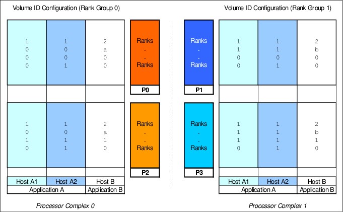
Figure 4-6 Application and extent pool-related volume layout example for four shared extent pools
The example that is depicted in Figure 4-7 on page 97 provides a numbering scheme that can be used in a FlashCopy scenario. Two different pairs of LSS are used for source and target volumes. The address group identifies the role in the FlashCopy relationship: address group 1 is assigned to source volumes, and address group 2 is used for target volumes. This numbering scheme allows a symmetrical distribution of the FlashCopy relationships across source and target LSSs. For example, source volume 1007 in P0 uses the volume 2007 in P2 as the FlashCopy target. In this example, use the third digit of the volume ID within an LSS as a marker to indicate that source volumes 1007 and 1017 are from different extent pools. The same approach applies to the target volumes, for example, volumes 2007 and 2017 are from different pools.
However, for the simplicity of the Copy Services management, you can choose a different extent pool numbering scheme for source and target volumes (so 1007 and 2007 are not from the same pool) to implement the recommended extent pool selection of source and target volumes in accordance with the FlashCopy guidelines. Source and target volumes must stay on the same rank group but different ranks or extent pools. For more information about this topic, see the FlashCopy performance chapters in IBM DS8000 Copy Services, SG24-8367.

Figure 4-7 Application and extent pool-related volume layout example in a FlashCopy scenario
|
Tip: Use the GUI advanced Custom mode to select a specific LSS range when creating volumes. Choose this Custom mode and also the appropriate Volume definition mode, as shown in Figure 4-8 .
|
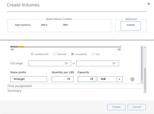
Figure 4-8 Create volumes in Custom mode and specify an LSS range
4.10 I/O port IDs, host attachments, and volume groups
Finally, when planning the attachment of the host system to the storage system HA I/O ports, you must achieve a balanced workload distribution across the available front-end resources for each workload with the appropriate isolation and resource-sharing considerations. Therefore, distribute the FC connections from the host systems evenly across the DS8900F HA ports, HA cards, and I/O enclosures.
For high availability, each host system must use a multipathing device driver, such as the native MPIO of the respective operating system. Each host system must have a minimum of two host connections to HA cards in different I/O enclosures on the DS8900F storage system. Preferably, they are evenly distributed between left side (even-numbered) I/O enclosures and right side (odd-numbered) I/O enclosures. The number of host connections per host system is primarily determined by the required bandwidth. Use an appropriate number of HA cards to satisfy high throughput demands.
With typical transaction-driven workloads that show high numbers of random, small-blocksize I/O operations, all ports in a HA card can be used likewise. For the preferred performance of workloads with different I/O characteristics, consider the isolation of large-block sequential and small-block random workloads at the I/O port level or the HA card level.
The preferred practice is to use dedicated I/O ports for Copy Services paths and host connections. For more information about performance aspects that are related to Copy Services, see the performance-related chapters in IBM DS8000 Copy Services, SG24-8367.
To assign FB volumes to the attached Open Systems hosts by using LUN masking, when using the DSCLI, these volumes must be grouped in the DS8900F volume groups. A volume group can be assigned to multiple host connections, and each host connection is specified by the worldwide port name (WWPN) of the host FC port. A set of host connections from the same host system is called a host attachment. The same volume group can be assigned to multiple host connections; however, a host connection can be associated only with one volume group. To share volumes between multiple host systems, the most convenient way is to create a separate volume group for each host system and assign the shared volumes to each of the individual volume groups as required. A single volume can be assigned to multiple volume groups. Only if a group of host systems shares a set of volumes, and there is no need to assign additional non-shared volumes independently to particular hosts of this group, can you consider using a single shared volume group for all host systems to simplify management. Typically, there are no significant DS8000 performance implications because of the number of DS8000 volume groups or the assignment of host attachments and volumes to the DS8000 volume groups.
Do not omit additional host attachment and host system considerations, such as SAN zoning, multipathing software, and host-level striping.
After the DS8900F storage system is installed, you can use the DSCLI lsioport command to display and document I/O port information, including the I/O ports, HA type, I/O enclosure location, and WWPN. Use this information to add specific I/O port IDs, the required protocol (FICON or FCP), and the DS8000 I/O port WWPNs to the plan of host and remote mirroring connections that are identified in 4.4, “Planning allocation of disk and host connection capacity” on page 73.
Additionally, the I/O port IDs might be required as input to the DS8900F host definitions if host connections must be restricted to specific DS8900F I/O ports by using the -ioport option of the mkhostconnect DSCLI command. If host connections are configured to allow access to all DS8000 I/O ports, which is the default, typically the paths must be restricted by SAN zoning. The I/O port WWPNs are required as input for SAN zoning. The lshostconnect -login DSCLI command might help verify the final allocation of host attachments to the DS8900F I/O ports because it lists host port WWPNs that are logged in, sorted by the DS8900F I/O port IDs for known connections. The lshostconnect -unknown DSCLI command might further help identify host port WWPNs, which are not yet configured to host connections, when creating host attachments by using the mkhostconnect DSCLI command.
The DSCLI lsioport output identifies this information:
•The number of I/O ports on each installed HA
•The type of installed HAs (SW FCP/FICON-capable or LW FCP/FICON-capable)
•The distribution of HAs across I/O enclosures
•The WWPN of each I/O port
The DS8900F I/O ports use predetermined, fixed DS8900F logical port IDs in the form I0xyz, where:
•x: I/O enclosure
•y: Slot number within the I/O enclosure
•z: Port within the adapter
For example, I0101 is the I/O port ID for these devices:
•I/O enclosure 1
•Slot 0
•Second port
|
Slot numbers: The slot numbers for logical I/O port IDs are one less than the physical location numbers for HA cards, as shown on the physical labels and in IBM Spectrum Control/Storage Insights, for example, I0101 is R1-XI2-C1-T2.
|
A simplified example of spreading the DS8000 I/O ports evenly to two redundant SAN fabrics is shown in Figure 4-9 . The SAN implementations can vary, depending on individual requirements, workload considerations for isolation and resource-sharing, and available hardware resources.

Figure 4-9 Example of spreading DS8000 I/O ports evenly across two redundant SAN fabrics
4.10.1 Fibre Channel host adapters: 16 Gbps and 32 Gbps
The DS8900F supports up to 32 Fibre Channel (FC) host adapters, with four FC ports for each adapter. Each port can be independently configured to support Fibre Channel connection (IBM FICON) or Fibre Channel Protocol (FCP).
Each adapter type is available in both longwave (LW) and shortwave (SW) versions. The DS8900F I/O bays support up to four host adapters for each bay, allowing up to 128 ports maximum for each storage system. This configuration results in a theoretical aggregated host I/O bandwidth around 128 x 32 Gbps. Each port provides industry-leading throughput and I/O rates for FICON and FCP.
The host adapters that are available in the DS8900F have the following characteristics:
•32 Gbps FC HBAs (32 GFC):
– Four FC ports
– FC Gen7 technology
– New IBM Custom ASIC with Gen3 PCIe interface
– Quad-core PowerPC processor
– Negotiation to 32, 16, or 8 Gbps (4 Gbps or less is not possible)
•16 Gbps FC HBAs (16 GFC):
– Four FC ports
– Gen2 PCIe interface
– Quad-core PowerPC processor
– Negotiation to 16, 8, or 4 Gbps (2 Gbps or less is not possible)
The DS8900F supports a mixture of 32 Gbps and 16 Gbps FC adapters. Hosts with slower FC speeds like 4 Gbps are still supported if their HBAs are connected through a switch.
The 32 Gbps FC adapter is encryption-capable. Encrypting the host bus adapter (HBA) traffic usually does not cause any measurable performance degradation.
With FC adapters that are configured for FICON, the DS8900F series provides the following configuration capabilities:
•Fabric or point-to-point topologies
•A maximum of 128 host adapter ports, depending on the DS8900F system memory and processor features
•A maximum of 509 logins for each FC port
•A maximum of 8192 logins for each storage unit
•A maximum of 1280 logical paths on each FC port
•Access to all 255 control-unit images (65,280 Count Key Data (CKD) devices) over each FICON port
•A maximum of 512 logical paths for each control unit image
An IBM Z server supports 32,000 devices per FICON host channel. To fully access 65,280 devices, it is necessary to connect multiple FICON host channels to the storage system. You can access the devices through an FC switch or FICON director to a single storage system FICON port.
The 32 GFC host adapter doubles the data throughput of 16 GFC links. When comparing the two adapter types, the 32 GFC adapters provide I/O improvements in full adapter I/Os per second (IOPS) and reduced latency.
Double bandwidth with 32 GFC HA
The latest DS8000 storage system support 32-gigabit fiber channel host adapters (32 GFC HA). This capability effectively doubles the bandwidth performance compared to 16 GFC HA. The 32 GFC HA is able to transfer data at 3.2 GBPS per port. It provides 2x bandwidth capacity at the port and the HA layer when compared to single 16 GFC HA. The 32 GFC HA ports are compatible with 16 GFC and 8 GFC infrastructure and can negotiate the transmission speed to 800 or 1600 MBPS depending on the Fibre Channel port they are connected to. With support for FICON, zHPF, and FCP protocols provided on an individual port basis, each port can support any one of these protocols so that a single 4-port HA card can have all supported protocols running concurrently.
Figure 4-10 on page 101 illustrates read/write performance with zHPF protocol

Figure 4-10 CKD/zHPF - 32 GFC vs. 16 GFC HA, Read/Write
Figure 4-11 illustrates Metro Mirror Bandwidth

Figure 4-11 Metro Mirror Link Bandwidth 32 GFC vs. 16 GFC HA
|
Note The above measurements were derived by running simulated workloads in a Lab environment. They are being provided purely to demonstrate comparative/indicative performance improvement between different HA and port types. Your current environment setup will determine the scope for performance improvements
|
General considerations about 16 and 32 GFC and I/O Ports
The following recommendations applies to 16 and 32 GFC and I/O Ports:
•Spread the paths from all host systems across the available I/O ports, HA cards, and I/O enclosures to optimize workload distribution across the available resources depending on your workload sharing and isolation considerations.
•Spread the host paths that access the same set of volumes as evenly as possible across the available HA cards and I/O enclosures. This approach balances workload across hardware resources, and it ensures that a hardware failure does not result in a loss of access.
•Plan the paths for the attached host systems with a minimum of two host connections to different HA cards in different I/O enclosures on the DS8900F storage system. Preferably, evenly distribute them between left (even-numbered) I/O enclosures and right (odd-numbered) I/O enclosures for the highest availability and a balanced workload distribution across I/O enclosures and HA cards.
•Use separate DS8900F I/O ports for host attachment and Copy Services remote replication connections (such as Metro Mirror, Global Mirror, and zGM data mover). If additional HAs are available, consider using separate HAs for Copy Services remote replication connections and host attachments to avoid any possible interference between remote replication and host workloads.
•Spread Copy Services remote replication connections at least across two HA cards in different I/O enclosures.
•Consider using separate HA cards for FICON protocol and FCP. Although I/O ports on the same HA can be configured independently for the FCP protocol and the FICON protocol, it might be preferable to isolate your z/OS environment (FICON) from your Open Systems environment (FCP).
Look at Example 4-2, which shows a DS8900F storage system with a selection of different HAs:
Example 4-2 DS8000 HBA example - DSCLI lsioport command output (shortened)
dscli> lsioport -l
ID WWPN State Type topo portgrp Speed Frame I/O Enclosure HA Card
================================================================================================
I0200 500507630A1013E7 Online Fibre Channel-SW SCSI-FCP 0 16 Gb/s 1 3 1
I0201 500507630A1053E7 Online Fibre Channel-SW FICON 0 16 Gb/s 1 3 1
I0202 500507630A1093E7 Online Fibre Channel-SW FICON 0 16 Gb/s 1 3 1
I0203 500507630A10D3E7 Online Fibre Channel-SW FICON 0 16 Gb/s 1 3 1
I0230 500507630A1313E7 Offline Fibre Channel-LW - 0 32 Gb/s 1 3 4
I0231 500507630A1353E7 Offline Fibre Channel-LW - 0 32 Gb/s 1 3 4
I0232 500507630A1393E7 Offline Fibre Channel-LW - 0 32 Gb/s 1 3 4
I0233 500507630A13D3E7 Offline Fibre Channel-LW - 0 32 Gb/s 1 3 4
I0240 500507630A1413E7 Online Fibre Channel-SW FICON 0 16 Gb/s 1 3 5
I0241 500507630A1453E7 Offline Fibre Channel-SW - 0 16 Gb/s 1 3 5
I0242 500507630A1493E7 Online Fibre Channel-SW SCSI-FCP 0 16 Gb/s 1 3 5
I0243 500507630A14D3E7 Offline Fibre Channel-SW - 0 16 Gb/s 1 3 5
I0300 500507630A1813E7 Offline Fibre Channel-LW - 0 32 Gb/s 1 4 1
I0301 500507630A1853E7 Offline Fibre Channel-LW - 0 32 Gb/s 1 4 1
I0302 500507630A1893E7 Offline Fibre Channel-LW - 0 32 Gb/s 1 4 1
I0303 500507630A18D3E7 Offline Fibre Channel-LW - 0 32 Gb/s 1 4 1
I0310 500507630A1913E7 Online Fibre Channel-SW SCSI-FCP 0 16 Gb/s 1 4 2
I0311 500507630A1953E7 Online Fibre Channel-SW FICON 0 16 Gb/s 1 4 2
I0312 500507630A1993E7 Online Fibre Channel-SW FICON 0 16 Gb/s 1 4 2
I0313 500507630A19D3E7 Online Fibre Channel-SW FICON 0 16 Gb/s 1 4 2
I0330 500507630A1B13E7 Online Fibre Channel-SW FICON 0 16 Gb/s 1 4 4
I0331 500507630A1B53E7 Offline Fibre Channel-SW - 0 16 Gb/s 1 4 4
I0332 500507630A1B93E7 Online Fibre Channel-SW SCSI-FCP 0 16 Gb/s 1 4 4
I0333 500507630A1BD3E7 Offline Fibre Channel-SW - 0 16 Gb/s 1 4 4
When planning the paths for the host systems, ensure that each host system uses a multipathing device driver and a minimum of two host connections to two different HA cards in different I/O enclosures on the DS8900F. Preferably, they are evenly distributed between left side (even-numbered) I/O enclosures and the right side (odd-numbered) I/O enclosures for highest availability. Multipathing additionally optimizes workload spreading across the available I/O ports, HA cards, and I/O enclosures.
You must tune the SAN zoning scheme to balance both the oversubscription and the estimated total throughput for each I/O port to avoid congestion and performance bottlenecks.
4.10.2 Further optimization
Sometimes the IBM support staff is asked if any further tuning possibilities exist with respect to HBAs, and paths. Although the impact is usually minimal, take the following hints and tips into consideration, whenever possible:
PPRC fine-tuning
For optimal use of your PPRC connections, observe the following guidelines:
•Avoid using FCP ports for both host attachment and replication.
•With bi-directional PPRC: Avoid using a specific adapter port for both replication output and input I/Os, rather consider to use each port in one direction only.
•When having a larger number of replication ports, assign even and odd LSS/LCU to different ports (example: With 4 paths, could use two only for all even LSSs to be replicated, and the other two for all odd LSSs to be replicated).
These guidelines help the adapters to reduce internal switching, what slightly increases their throughput for PPRC.
I/O Bay fine-tuning
The DS8000 models use specific algorithms to distribute internal CPU resources across the I/O Bays, depending on the specific submodel and cores available. As a result of this, some configurations are more favorable than others, and the following guidelines apply:
•Balance your host attachments well by spreading across all available I/O Bays.
•Balance your PPRC connections well by spreading them across all available I/O Bays.
•Avoid to order a DS8000 with many cores (DS8000s with 1 TB and larger caches) but then with only 2 I/O Bays in a frame. That also means for instance, if it is a stronger 2-frame storage system and it is decided that just 4 I/O Bays in total are enough, have these all in one frame.
•Spreading a particular workload over host adapters in only either the top bays of both frames, or only the bottom bays of both frames, would also not lead to the most optimal result – hence spread each bigger load (attachment/core switches, PPRC) across all the various rows of bays that you have.
•These guidelines would also apply in case of incoming PPRC load (Secondary DS8000), or when doing an even/odd load split with the PPRC paths as mentioned in the PPRC section. So if you do such a split, spread out the paths across all I/O Bays in each case, like across the 4 bays in one frame.
4.11 Documentation of the logical configuration
You can use the DS Storage Manager GUI to export information in a spreadsheet format (CSV file). Figure 4-12 the shows the export of the GUI System Summary. The resulting spreadsheet file contains a lot of detailed information, such as cache and drives installed, HAs installed, licenses installed, arrays created and extent pools, all volumes created, hosts and users, and code levels. You can also consider this function for regular usage.

Figure 4-12 Export System Summary
..................Content has been hidden....................
You can't read the all page of ebook, please click here login for view all page.