


Geographic Discovery and Mapping
This chapter features a scenario that describes how to automatically include and use Geographic Information System (GIS) data for network devices that are discovered by the Network Manager. Also described is how Geographic mapping can help operators and other users visually orient problems that are based on location.
This early-release capability is available for download and is fully supported by the Development team. For more information about the link to download the distribution package, see 3.5, “Summary” on page 81.
This chapter includes the following topics:
3.1 Scenario description
This scenario describes how you can use the Geographic maps to gain an at-a-glance understanding of where the devices are and how they are connected, including the active status of the devices and links. It is also an alternative mechanism that can be used to drill down for more information about devices and links.
3.1.1 Business value
Geographic mapping shortens time to triage events or diagnose problems by understanding the geographic layout around the issue intuitively. The geographic orientation helps operators align outside knowledge with the network problems they are seeing. It is helpful not only for location sensitive devices on cell towers, but also to see status across the network backbone and core networks around the world. Operators can quickly see all the device details for alarms, inventory, contacts, and connections at their fingertips. Administrators can set up flexible views to match areas of responsibility that are tied to operators based on location (latitude-longitude dimensions), device types, services, and so on.
3.2 Geographic map basics
Before describing the scenario steps, we describe how to use the Geographic map in Network Manager.
3.2.1 Use of the Geographic map
The Geographic map displays the individual devices according to their latitude and longitude values. Those devices that are closely collocated are aggregated into a Building.
Complete the following steps to use the Geographic map:
1. Right-click the Building site icon to see the list of all devices there, including their status, event counts, connectivity, and details.
2. Use the right-click menu on any row to use the standard context tools for browsing to other topology views, structure browser, Top Performers, or the diagnostic tools, such as Ping and Trace route, as shown in Figure 3-1.
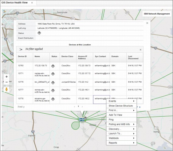
Figure 3-1 Right-clicking building site link
3. You can also right-click a link to show all of the connections it represents. Right-click a single row to perform actions on that link, as shown in Figure 3-2.
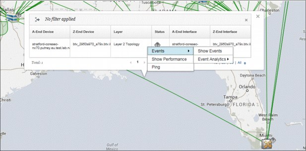
Figure 3-2 Right-click a single row
4. The device status is taken from the active events and aggregated in the case of the Building site. Use the Map Configuration icon at top left to control what event severities to include.
5. Connectivity is also aggregated from Buildings and by right-clicking the link, a table of all the links and their status is shown. Use the Map Configuration icon to control what connectivity layers to display.
The Map Configuration icon can also be used to dynamically filter the devices on display by Network Manager domain and device type.
3.2.2 Use of the Health view
Access this page by click in the DASH task menu Incident → GIS Device Health View, as shown in Figure 3-3.

Figure 3-3 GIS Device Health view
This page contains the Geographic map and an Event Viewer, which shows events in context for the device or Building site that is clicked. By default, the page layout features a horizontal split that shows more event columns, but with a narrower map view. If you prefer, you can edit the DASH page and drag the windows into a vertical split (see Figure 3-3) for a larger map area on wide-screen monitors.
3.2.3 Browsing to the Geographic map
If you are looking for geospatial information about a device from one of the topology views, you can browse to the Geographic map from the Hop View, Path View, or a Network View. Right-click the device and click Find in → Geographical Map. A new browser page opens with the Geographic map, as shown in Figure 3-4.
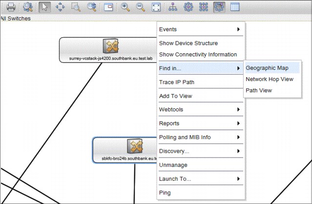
Figure 3-4 Browsing the to Geographic map
3.2.4 Use of Network Views for the Geographic map
You can use the inter-portlet events to control the Geographic map from the same Network Views tree that is used by the Network Health Dashboard.
This view is similar to the Network Health page, but uses the Geographic map instead of the network view topology. In this scenario, an operator can select a network view to show areas of responsibility or other grouping. As with the Network Health Dashboard, the network view tree works off the default bookmark for each user, which makes it easier for each user to create a custom set of useful network views.
Click a view to change the context of the geographical map and all events for devices in that view. Click a device or Building site icon to see events for that device or site, only (see Figure 3-5 on page 73).
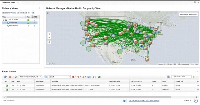
Figure 3-5 Custom Geographic Views page
Building the Geographic Views page
Complete the following steps to build the custom page for the Geographic Views:
1. Click Console Settings → Pages.
2. Click New Page and enter a name for the page. In this example, the name Geographic Views is used.
3. Click Location and drag the Geographic Views menu item that is in the console/Incident/Network Geography directory, as shown in Figure 3-6.

Figure 3-6 Menu location for the new Geographic Views
4. Select Proportional Layout and then, click OK.
We select each of the three widgets for this page in turn and drag and expand each widget into position.
5. Click Network Manager Widgets and drag the Dashboard Network Views onto the workspace and expand it (as shown in Figure 3-5 on page 73) or to your own design. Then, by using the menu at the top left, select Home to return to the widget Home level.
6. From the Home level, click Network Manager (Experimental) Widgets and drag the GIS Device Map widget into place and expand, as appropriate. Return to the widget Home.
7. Click Netcool/OMNIbus Widgets and drag the Event Viewer widget into place.
Your page is complete now. The final step for to set the wiring events so that the contextual changes work as wanted.
8. Select the Event Viewer widget and then, from the Widget pull-down menu on the tool bar at the top of the page, select the Events, as shown in Figure 3-7.
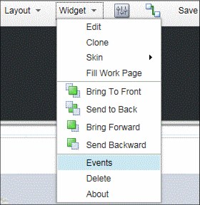
Figure 3-7 Set Wiring Events for widgets
9. Adjust the selected published and subscribed events to match the settings that are listed in Table 3-1. No changes are necessary for the other two widgets.
Table 3-1 Configuration table
|
Widget
|
Published Events
|
Subscribed Events
|
|
Event Viewer
|
(Uncheck NodeClickedOn)
|
showEvents
NodeClickedOn
|
|
GIS Device
|
showEvents
|
NodeClickedOn
|
|
Dashboard Network Views
|
NodeClickedOn
|
-
|
10. Click Save and Exit. The widget now can be tested.
|
Note: The Network View uses bookmarks only, so you must click Incident → Network Views first to set up a default bookmark and add the views from the Library. If completed this task for the Network Health Dashboard, it does not need to be repeated. For more information, see this website:
|
Later for production, you might want to edit this page to set appropriate security roles.
3.3 Scenario topology
The solution that is used in this scenario includes system components that are installed on the following host names:
•hostname1:
– OMNIbus WebGUI 8.1
– Network Manager GUI 4.2
– Network Health Dashboard 4.2 (optional)
•hostname2: ITNM 4.2 core
•hostname3: DB2 10.5
The capability that is described in this chapter is not included with Network Manager. For more information about where to download, install, and set up the distribution package, see 3.4, “Scenario steps”.
For this scenario, we use Google Maps API.
For more information about system components and default settings that were used in the test environment, see Chapter 1, “IBM Netcool Operations Insight overview” on page 3.
3.4 Scenario steps
This section describes that steps that are used to deploy and configure Geographic maps that show devices and sites that are overlaid and aggregated on a world map.
This early-release capability is available for download and is fully supported by the Development team. For more information about downloading the distribution package, see 3.5, “Summary” on page 81.
For convenience, start by making the distribution package available to the Network Manager core server, DB2 server, and the GUI server.
From the distribution package, we use the files that are shown in Example 3-1 on page 76 and any of their supporting files. The files that are shown in Example 3-1 on page 76 might change in future distribution updates; therefore, refer to the documentation and modify these steps accordingly.
Example 3-1 Files in the distribution package
ncp_gis.war
nm_rest.war
bin/db2/modifyGISTables.sql
bin/db2/update_geo_location.sh
bin/install.sh
samples/GeoByLookup/data/core_lat_long.csv
samples/GeoByLookup/stitchers/ACMEDeviceLocationEnrich.stch
samples/GeoByLookup/stitchers/PopulateDNCIM_CustomGeography.stch
etc/tnm/tools/findInGeoMapByDevice.xml
etc/tnm/tools/findInGeoMapByView.xml
etc/tnm/menus/ncp_findIn_submenu.xml
etc/tnm/menus/ncp_gis_device_menu.xml
etc/tnm/menus/ncp_gis_link_menu.xml
3.4.1 Updating network connectivity and inventory model database
Update the NCIM schema for the standard ncim.geographicLocation table that is included with Network Manager 4.2 GA.
|
NCIM topology database: The Network Connectivity and Inventory Model (NCIM) topology database is a relational database that Network Manager uses to consolidate topology data about the physical and logical composition of devices, layer 1, layer 2, and 3 connectivity, routing protocols, and network technologies, such as OSPF, BGP, and MPLS Layer 3 VPNs.
|
Run the following command on the db2 server:
bin/db2/update_geo_location.sh NCIM db2inst1 <password>
Where:
•NCIM is the database name
•db2inst1 is a database instance user with privileges to modify the schema
•<password> is the db2inst1 password
3.4.2 Installing the Geographic maps on DASH
This task is performed on the GUI server where the Network Manager GUI is installed.
Installing the GIS Device Map widget
Before installing the widget, you must edit the defaults at the top of the bin/install.sh file to match your environment.
For example, the text in bold might need to be changed:
JAZZSM_PROFILE=/opt/IBM/netcool/JazzSM/profile
JAZZSM_CELL=JazzSMNode01Cell
SERVER_NAME=server1
CMD=RESTART
GIS_CTX_ROOT=/ibm/console/ncp_gis
REST_CTX_ROOT=/ibm/console/nm_rest
USERNAME=smadmin
PASSWORD=netc00l
Run the bin/install.sh -d command. You must run this command from the top-level directory of the distribution kit.
Use -d to deploy for the first time and -r to redeploy or upgrade the war file.
When it finishes, log in to DASH and ensure that you have a new menu section under Incident that is called Network Geography with the following two items:
•GIS Device Health View
•GIS Device Map
Geographic map context menus
Copy the files into place that add the navigation to the Geographic map from the context menus.
The Geographic map context menus are defined in the following files:
•ncp_gis_device_menu.xml
•ncp_gis_link_menu.xml
•ncp_findIn_submenu.xml
From the distribution package, find and copy the following files:
[root@ncrobitm tnm]# cp menus/ncp_gis* /opt/IBM/netcool/gui/precision_gui/profile/etc/tnm/menus/
[root@ncrobitm tnm]# cp menus/ncp_findIn_submenu.xml /opt/IBM/netcool/gui/precision_gui/profile/etc/tnm/menus/
Copy the following supporting tools files:
tools/findInGeoMapByDevice.xml
tools/findInGeoMapByView.xml
[root@ncrobitm tnm]# cp tools/findInGeo* /opt/IBM/netcool/gui/precision_gui/profile/etc/tnm/tools/
3.4.3 Custom enrichment for the geographical data
The task that is described in this section is performed on the Network Manager core server.
There are various ways to customize Network Manager’s discovery process to enrich devices with the geographical location data. We chose a method that starts with a flat file as the source of the data (core_lat_long.csv). We import this file manually into a database custom staging table. During discovery, the two custom stitchers that are provided merge this data into the standard NCIM tables in Network Manager 4.2.
We use the core_lat_long.csv file as the original source of the location data per IP address for this scenario.
|
Tip: This method is convenient and helps you to get started quickly. For production, you might make changes to automatically maintain this data in the staging table from your source data. Also, you might consider the use of the EntityName instead of the IP address to index the device.
|
Creating the staging SQL table
Create an SQL file (for example, name it createAcmeGeoLocation.sql), with the following command:
CREATE TABLE NCIM.ACMEGEOLOCATION (
IP VARCHAR(255) NOT NULL,
ADDRESS VARCHAR(255),
CITY VARCHAR(255),
STATE VARCHAR(255),
COUNTRY VARCHAR(255),
LATITUDE DECIMAL(10 , 8) NOT NULL DEFAULT 0,
LONGITUDE DECIMAL(11 , 8) NOT NULL DEFAULT 0
);
Use the following command to apply this file:
db2batch -d NCIM -a db2inst1/<password> -f createAcmeGeoLocation.sql
Where:
•NCIM is the database name
•db2inst1 is a database instance user with privileges to create the table
•<password> is the db2inst1 password
Importing the data to the staging table
Import the data in core_lat_long.csv into the NCIM.ACMEGEOLOCATION table by running the commands that use the same database account, as shown in Example 3-2.
Example 3-2 Importing the data to the staging table
db2 => connect to NCIM
Database Connection Information
Database server = DB2/LINUXX8664 10.5.3
SQL authorization ID = DB2INST1
Local database alias = NCIM
db2 => import from core_lat_long.csv of del insert into ncim.ACMEGEOLOCATION(ip,address,city,state,country,latitude,longitude)
SQL3109N The utility is beginning to load data from file "core_lat_long.csv".
SQL3110N The utility has completed processing. "155" rows were read from the
input file.
SQL3221W ...Begin COMMIT WORK. Input Record Count = "155".
SQL3222W ...COMMIT of any database changes was successful.
SQL3149N "155" rows were processed from the input file. "154" rows were
successfully inserted into the table.
Number of rows read = 155
Number of rows skipped = 0
Number of rows inserted = 154
Number of rows updated = 0
Number of rows rejected = 1
Number of rows committed = 155
db2 => quit
|
Tip: As shown in Example 3-2 on page 78, the core_lat_long.csv file contains 154 locations and a header line, which is correctly rejected by the db2 command.
|
Deploying the custom geographic stitchers
Complete the following steps to deploy the custom geographic stitchers:
1. Find the following stitchers in samples/GeoByLookup/stitchers/:
– ACMEDeviceLocationEnrich.stch
– PopulateDNCIM_CustomGeograpghy.stch
2. Copy the stitchers to $NCHOME/precision/disco/stitchers/DNCIM/.
3. Edit $NCHOME/precision/disco/stitchers/DNCIM/InferDNCIMObjects.stch to add a line to run the custom ACMEDeviceLocationEnrich.stch stitcher:
// Build the WLAN model
if(wlanEnabled <> NULL)
{
ExecuteStitcher('PopulateDNCIM_WLAN', domainId, isRediscovery, dynamicDiscoNode);
}
delete(wlanEnabled);
// CUSTOM (5/4/2016): Enrich GEO Location data
ExecuteStitcher('ACMEDeviceLocationEnrich', domainId, isRediscovery, dynamicDiscoNode );
|
Important: If multiple domains are used but the geographic data is imported to only one of the domains, create a domain-specific version of this stitcher; for example, InferDNCIMObjects.SBK.stch, assuming SBK is your domain name.
|
Running a discovery
You are now ready to run a discovery. After the discovery is run, check whether the ncim.geographicLocation table was populated with the location data for devices that match those devices in core_lat_long.csv. This table is a standard NCIM table and you might decide not to populate all of the columns.
3.4.4 Registering for the Google Map Key and Client ID
This widget is based on an integration with the Google Maps API. As a deployer and user of this solution, you must ensure that you are compliant with the Terms of Use for Google Maps. Complete the following steps:
1. For Google, obtain a valid key from this website:
2. Search for the Google Maps JavaScript API and register for a Key/Client ID. This file uses the following format:
AIzaSyBPS0oWeQkjVS1ogd3X6GRh8MPjqIyRKCq
3. Add this key to the config.json file at:
/opt/IBM/netcool/JazzSM/profile/installedApps/JazzSMNode01Cell/isc.ear/ncp_gis.war/resources/config.json
The default config.json file without the license key is shown in Example 3-3.
Example 3-3 Default config.json file without the license key
"mapProvider": {
"baseLayers": [
{
"baseLayerName": "Google",
"baseLayerURL": "https://maps.google.com/maps/api/js?libraries=visualization,drawing,geometry&v=3.exp"
The config.json file after the key is applied (note the ‘&’) is shown in Example 3-4.
Example 3-4 After the key is applied
"mapProvider": {
"baseLayers": [
{
"baseLayerName": "Google",
"baseLayerURL": "https://maps.google.com/maps/api/js?libraries=visualization,drawing,geometry&v=3.exp&AIzaSyBPS0oWeQkjVS1ogd3X6GRh8MPjqIyRKCq"
As distributed, there is no default license applied. When the user starts the Geographic map in DASH, the warning that is shown in Example 3-8 is displayed.

Figure 3-8 Invalid license
3.4.5 No known problems status
By default, the status is “unknown” if there are no events for a device and it is shown with a question mark. You can change this status so that no active events means “no known problems” and marked as green.
Complete the following steps:
1. Edit the config.json file that is in /opt/IBM/netcool/JazzSM/profile/installedApps/JazzSMNode01Cell/isc.ear/ncp_gis.war/resources/config.json
2. Find “sevColours” and change the name pair “unknown” : “grey” to the value “green”, as shown in Example 3-5.
Example 3-5 Find “sevColours” and set “unknown” to “green”
"sevColours" : {
"unknown" : "green",
"clear" : "green",
3. Change the unknown icon to be the same as the clear icon:
a. Go to the directory:
/opt/IBM/netcool/JazzSM/profile/installedApps/JazzSMNode01Cell/isc.ear/ncp_gis.war/resources/common_assets/status_icons
b. Run the following commands:
cp unknown.png unknown.png.orig
cp clear.png unknown.png
3.5 Summary
This chapter described how to set up the Geographic mapping scenario for ITNM 4.2 with DASH in a test environment. Various use cases also were described to show the value for operators and others, including a big wall status map.
This early-release capability is available for download. At the time of this writing, the Sprint 1 version was used. For more information about the latest distribution packet, see this website:
..................Content has been hidden....................
You can't read the all page of ebook, please click here login for view all page.