Chapter 7

GENEXP-LANDSITES: a 2D Agricultural Landscape Generating Piece of Software

7.1. Introduction

The GENEXP-LANDSITES software is a two-dimensional (2D) random agricultural landscape generator, first developed in 2003 as part of a study on the coexistence of genetically modified crops with traditional crops. It uses tools stemming from spatial statistics and algorithmic geometry. Its main goal was to provide agricultural landscape maps to test the role of certain characteristics of these landscapes faced with transgene dissemination. Indeed, until the beginning of the noughties, agrobiologists worked with dissemination models that were developed at the level of a few fields and lacked any real data allowing them to scale up to the level of a landscape, even though various studies had shown it was necessary [ANG 02]. On a practical level, GENEXP-LANDSITES offers the agrobiologist user a set of methods to generate and describe landscapes – field pattern and land use – which are then used as input for gene flow models.

The following chapter follows the main outline of our book: a context description (section 7.2), a presentation of the major functionalities of GENEXP-LANDSITES, and the description of a case study (sections 7.3 and 7.4), the architecture details (section 7.5) and a few elements about the user and developer community (section 7.6).

7.2. Context

Landscape¹ simulation has been an important field of research for over 20 years in landscape ecology, and, more recently, in agronomy. The goal of landscape ecology is to study the role of landscape structures faced with ecological dynamics [TUR 91]. Simulation methods can be divided into three groups: geostatistical models, neutral landscape models, and explicit process models [SAU 00]. Geostatistical models are based on spatial data interpolation methods [GOT 96]. In explicit process models, the landscape is the result of modeled ecological processes (dispersion, competition, etc.). On the contrary, neutral landscape models (NLM, as described by [GAR 87]) provide random landscape structures which can serve as references to compare with real landscape, or which allow us to test the effect of certain landscape structures, such as, for instance, the habitat fragmentation, on ecological processes [GAR 87, GAR 91, WIT 97]. The NLM are essentially based on raster approaches, land use (often limited to two categories) is randomly allocated to pixels which are then grouped to create fragments of space with similar use. To obtain more “realistic” landscapes with various categories, classification [SAU 00] or fractal [HAR 02] approaches have also been developed. Approaches based on tessellations were recently suggested to simulate geometrically shaped landscapes, forest landscapes, or agricultural landscapes [GAU 06a, GAU 08].

Landscape models were frequently used to help manage forests [KUR 00, LIU 98]. In the fields of agricultural land management and agronomy, these models are less common. Spatial models have notably been used to simulate crop distribution within a farm or a piece of land [CAR 02, LEB 98] to understand the impact of agriculture on ecological issues (such as drinking water pollution) or to plan more favorable spatial organizations. Closer to what has been done in ecology, some studies have explored the link between agricultural practices (crop rotation, land consolidation, etc.) and ecological processes thanks to explicit process models [AVI 07, GAU 06b]. All these models are based on real data such as spatial distributions of fields, physical characteristics of landscapes (soil conditions, slope, etc.), or crop distribution on the studied zone. Beside a few recent works [GAU 08], there is no neutral model in those fields such as the ones developed in landscape ecology. These models are interesting for various reasons. On the one hand, real data are not always available or can be too specific, thus restricting the scope of the model's results. on the other hand, prospective studies can be based on new landscape configurations which did not exist before. Finally, neutral landscape models can be used to test a process model's sensitivity to agricultural land spatial variability.

Beyond the structure simulation, agricultural landscape models tackle the simulation of land use in various ways. In most landscape models, land use is randomly allocated on the modelized area according to a law of probability: for example, in binary landscapes, each plot has a probability of being planted with a specific crop that depends both on its area and a value p matching the crop. When various land uses are modeled, each land use is matched to a probability p_c so that Σ_cp_c = 1. There have been various methods suggested to improve the purely random approach. In [GAU 06a], the authors introduced a Gibbs process to model interactions between pairs of adjacent fields. The landscape mosaic can be more or less heterogeneous depending on the parameter values of this model. Other processes can be used, based on the statistical study and spatiotemporal pattern characterization of real agricultural mosaics [CAS 07, CAS 08]. Moreover, stochastic rules of adjacency can be learnt from real sets of data, as [MAR 06] suggested it. In this study, the hidden Markov chains were implemented on land use spatiotemporal data. Deterministic approaches can also be used, especially to study the effects of decision rules or evolution scenarios of land use [CAR 02, GAU 06b].

In France, we can currently see a rise in landscape models to deal with various issues. For example, researchers participating in the RECORD² platform are considering developing a 2D landscape scale to represent the landscape distributions of crop systems. Other models focus more on modeling the physical process and include soil and slope characteristics – often based on real data, which can be distorted: a virtual landscape model is described in [SOR 08], for instance. We can also mention the APILand tool developed by the INRA SAD-Paysage unit in Rennes [BOU 10]. The GENEXP-LANDSITES model presented here has been developed to study the coexistence of genetically modified organism (GMO) crops with traditional crops [ADA 07, LEB 09]. Agrobiologists wanted to study in more detail the role of agricultural landscape structure in the dissemination of transgenes (originating from GMO) thanks to wind, regrowth or mechanical transportation. Moreover, they tried to characterize landscapes in which the risk is limited [COL 09b, LAV 08]. The elaboration of GENEXP-LANDSITES thus happened originally within the framework of the research project “Modeling transgene dissemination at the scale of agricultural landscapes” (answering the call to tender for “OGM Impact” put out by the French Research Ministry between 2003 and 2006) and required a panel of experts (in biology, statistic, agronomy, and computer science). Computer science students implemented the first versions [DEL 04, GUE 03]. GENEXP-LANDSITES's Gnu Public License was then filed with the Program Protection Association³. Further releases were carried out thanks to student internships with no specific funding [KAL 07, MOR 06]. However, the constant interest expressed by agrobiologists recently allowed us to obtain funding within an INRA-INRIA call to tender. The PAYOTE project “Agricultural land and landscape models to study the agro-ecological process” (2009-2010)⁴ brought together a set of INRA and INRIA researchers to think about these issues. These reflections led to new development in 2009 and 2010, to strengthen and expand GENEXP-LANDSITES's functionalities [BRO 09, KOS 10].

7.3. Major functionalities

The GENEXP-LANDSITES software is not a geographical information system but a 2D virtual agricultural landscape generator. This means it does not manage spatial information about the landscapes – even if it can use certain data extracted from real landscapes – but it allows us to create more or less realistic field pattern maps and stands as a complementary tool for GIS. It has two main functionalities: field pattern simulation and cropping pattern simulation. It relies on coupling with the R piece of software to offer more functionalities, concerning point process simulation and spatial analysis. We will thus successively present: (1) point generation, which requires R's libraries, (2) field pattern simulation, based on space tessellation methods, (3) cropping pattern simulation, and (4) post-production and spatial analysis.

7.3.1. Point generation

To generate points (or tessellation seeds), GENEXP-LANDSITES relies on the libraries of the piece of statistical software R and more specifically on its spatial statistics library, SPATSTAT [BAD 05]. There are more than one option possible: random approaches based on neutral processes (Poisson processes) or on processes fitted to the characteristics of a real landscape. Thus the barycenters of the fields of a real landscape can be used as seeds for virtual landscapes. They can also be used to asses a distribution model of plot barycenters [ADA 07], allowing us to control a certain variability in their number and location in virtual landscapes (Figure 7.1).

7.3.2. Field pattern simulation

The main goal of GENEXP-LANDSITES is to offer different field pattern generation algorithms. We are showcasing two here: the Voronoï diagrams and a random rectangular tessellation.

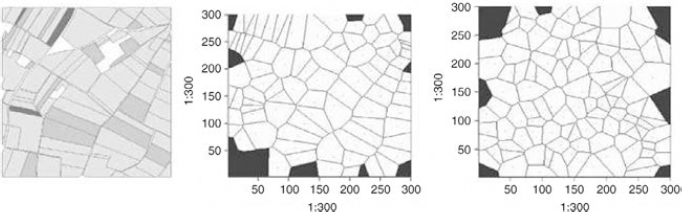
Figure 7.1. Three field patterns: (left) real landscape, (middle) simulated – Voronoï diagrams – landscape based on real barycenters, (right) simulated landscape based on simulated barycenters

7.3.2.1. Voronoï diagrams

A Voronoï diagram is a partition of the Euclidean plane ², generated from a set of points E, called “sites” or “seeds”. Each seed g₁ matches an element p_l of this partition, defined as the subset of the points in the plane which are closer to g₁ than to any other seeds in E [OKA 00]. The partition is thus built around as many polygons as there are seeds. These polygons are called “Voronoï polygons” and are convex. Their edges are thus made of the points which are equidistant from two seeds (Figure 7.2(a)).

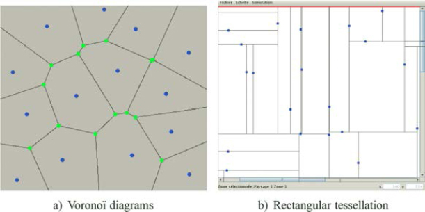
Figure 7.2. Two tessellations built on point seeds: a) Voronoï diagrams and b) rectangular tessellation with T vertices

On a practical level, GENEXP-LANDSITES first builds the Delaunay triangulation by using the 3D convex hull algorithm (see Algorithm 7.1, and also [OKA 00]) and then determines the matching Voronoï diagram. The algorithm insertion is derived from [ORO 98].

Algorithm 7.1 3D Convex hull

Input: a set P = {p₁, p₂,. . ., p_n} of n seeds whose coordinates are (x_i, y_i) for any i ∈ [1, n]

Output: Delaunay triangulation on the set P

Process:

Step 1: build the set P* = {p*₁, p*₂, . . . , p*_n} in dimension 3 in which the two first coordinates of p*ⁱ are those of p_i and the third coordinate is x_2i + y₂ⁱ

Step 2: build the convex hull C(P*) of P* in a 3 dimensional space.

Step 3: project all the lower bifaces of C(P*) in the original 2 dimensional space on a parallel with the third axis; flip the resulting diagram.

Each polygon is then identified as a field of the simulated agricultural landscape. The result can be easily linked to the structure of a real landscape; we can, for example, obtain the seeds from the barycenters of the real landscape fields.

7.3.2.2. Random rectangular tesselation

A rectangular tessellation allows us to divide the Euclidean space into jointed rectangular shapes which do not overlap. By eliminating the simple case where rectangles are defined by two orthogonal sets of parallel lines, we can focus on a tessellation where the vertex of a triangle is always on the side of another rectangle (T vertices and not X vertices, see Figure 7.2(b)). GENEXP-LANDSITES implements a method described in [MAC 96]. The algorithm principle (see Algorithm 7.2) is to generate the sides of the rectangles from a set of points: from each point start two opposed segments which are parallel to the x-axis or the y-axis. When two segments meet, the longer one stops. We then have a number of rectangles equal to the number of points minus one.

Algorithm 7.2 Rectangular tessellation

Input: a set P = {p₁, p₂,...,p_n} of n seeds; each p_i has a direction d₁, vertical or horizontal, with probabilities of 1/2, 1/2.

Output: a list of n couples of points (radius extremities). Process:

Step 1: for each couple (p_i, d_i), the adjacent d_j orthogonal to d_i are identified; they are potential blockers.

Step 2: for each couple (p_i, d_i), a radius is drawn along the direction d_i until it reaches its closest blocker.

Step 3: the isolated (unfinished) radii are dealt with sequentially. The current RC radius is prolonged towards its closest blocker, RB. There are then three possibilities:

(i) RB is already finished (on another line); RC is prolonged until the next blocker;

(ii) RB has not reached RC's line: RC is then suspended and RB becomes RC (the current radius);

(iii) RB went beyond RC's line: RC ends on RB and leaves from the list of isolated radii.

Variations on this algorithm have also been implemented by playing on the axis direction to obtain diversely oriented rectangles or non-rectangular parallelograms [KOS 10]. When it comes to the link between this type of tessellation and landscapes, we can see that the initial points are placed on any side of the rectangles. There is thus no obvious link between the tessellation seeds and remarkable points (barycenters, field vertices) of a landscape.

7.3.3. Cropping pattern simulation

GENEXP-LANDSITES allows us to randomly allocate land use to simulated fields, on the basis of a distribution of probabilities representing a cropping pattern (such as 50% corn, 30% wheat, etc.). GENEXP-LANDSITES also allows us to simulate the evolution of this cropping pattern over time, and the succession of crops on the different fields. The crop sequences are represented with Markov models (MM) or hidden Markov models (HMM) in two different ways. The models can be manually built as in [CAS 08], or we can obtain them thanks to sets of real data through the CARROTAGE software [LEB 06]. This stochastic data mining software works on temporal sequences of agricultural land use and represents these sequences with an HMM made of two states: a container state (written as “all” in Figure 7.3) representing a land use distribution similar to a cropping pattern, and a “Dirac” state in which there is only one type of land use (see “wheat”, “corn”, “rapeseed” in Figure 7.3).

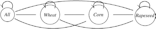
Figure 7.3. The different states of an HMM representing sequences dominated by rapeseed, wheat, corn

7.3.3.1. Stationary method

This method uses transitional mean probabilities (also called a priori probabilities) between the states of an HMM which has already been learnt from real data gathered over an agricultural land [MAR 06, LEB 06]. In a first time t, GENEXP-LANDSITES allocates crops to the fields according to a given distribution which represents crop rotation. In a second time t + 1, land use is simulated by using the a priori transitional probabilities between crops calculated for this HMM with CARROTAGE. Land use is obtained through a random selection based on three multinomial distributions matching the transitions and distributions. The process can be repeated over n periods of time to simulate stable successions over time.

7.3.3.2. Taking into account succession changes

This method uses the diagram representing probabilities over time (also called a posteriori probabilities) of the transitions between states over a given period of time. Figure 7.4 shows a diagram for an open plain of cereal crops which is dominated by a 4-year crop rotation cycle of rapeseed-wheat-sunflower-wheat. This figure shows an increase in wheat monoculture since 1996 for which the HMM a priori probabilities do not account. The HMM used (see Figure 7.3) has the following individualized states: sunflower, winter grain (wheat), rapeseed, pastures, corn, not surveyed, or constructs. The state noted as “?” corresponds to the container state covering all the other land uses. Thanks to these a posteriori probabilities, we can simulate successive land uses with the same dynamics and over the same period of time as a given region by using multinomial distributions similar to the method described earlier.

7.3.3.3. Future changes

We are currently working on two major changes: (i) spatial allocation of land use with a Gibbs process similar to the one suggested in [GAU 06b], (ii) temporal and spatial allocation – to keep consistency among the landscapes simulated over time – thanks to classified HMM [LAZ 09].

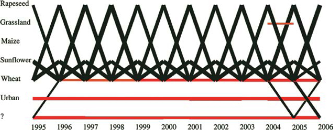
Figure 7.4. Temporal evolution of crop successions (dominated by rapeseed, wheat, sunflower) with the a posteriori probabilities given by an HMM

7.3.4. Post-production, spatial analysis, and formats

7.3.4.1. Post-production

GENEXP-LANDSITES allows for a certain number of postproductions on the generated landscapes. We can mention, among others:

• – diminishing fields that spill over the borders of the landscape (especially for Voronoï diagrams);
• – deleting segments that are too small (point merger, see Figure 7.5);
• – deleting fields that are too small or merging them with an adjacent field.

7.3.4.2. Spatial analysis

As for the spatial analysis, we have basic functions: field number, field area, number of sides, perimeter, barycenter, and shape index. The matching statistics are displayed as a histogram for a landscape and/or a boxplot if we wish to compare landscapes.

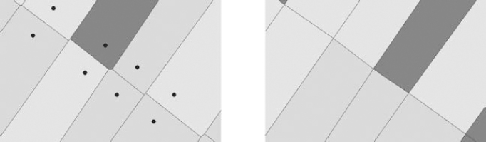
Figure 7.5. Post-production: aligning segments by merging points (left, initial Voronoï diagram, right, after post-production)

Using the R's SPATSTAT library [BAD 05] enables us to calculate other parameters, such as the distance of barycenters to their nearest neighbor (see below, in the case use).

7.3.4.3. Formats, import, and export

GENEXP-LANDSITES was originally devoted to producing maps for specific software. It can therefore manage these specific formats as well as GIS (shapefile format), image formats and XML formats.

7.4. Case uses

The GENEXP-LANDSITES software currently generates field pattern maps to be used by two gene flow models dealing with different crops. Colbach [COL 09a] is a multiannual model allowing us to predict the level of adventitious presence in rapeseed crops (e.g. the level of GMO in non-GMO crops or the level of erucic acid in varieties 00) to a field pattern made of tilled land and spaces outside the fields such as roadsides, a sequence of crops on each field and associated tillage techniques. The whole set is defined by the user at the model input. Angevin et al. [ANG 08] simulates gene dissemination of corn in a spatially heterogeneous space at the scale of a full crop year. It does not take the crop sequences and grain transfers into account, since they are not persistent from one crop year to the other in European climates.

The aim is to study the effect of field pattern (shape, location, and field area distribution) on gene flow, or it can operate on real field pattern or on field pattern whose shape will have been modified (e.g. by using the Voronoï tessellation on real field barycenters) or the shape and location of fields (for instance, by using a Voronoï tessellation on random seeds or a rectangular field pattern). Figure 7.6 shows a chain of tools and data required to implement such a study. Later on, GENEXP-LANDSITES can be used to study other spatialized ecological processes.

We will describe below in more detail the main stages of a study carried out with, and based on, real landscape data and on a set of simulations generated in GENEXP-LANDSITES. Detailed studies are described in [ADA 07, COL 09b, LAV 08, LEB 09].

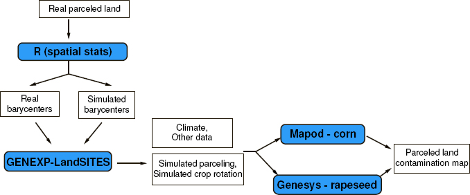
Figure 7.6. Chain of different models and data to simulate the flow of genes in an agricultural landscape

Suppose datasets from real field patterns are available. The biologist can use them as input data for the gene flow model. However, his/her goal is to study the effects of the variation of certain characteristics of these landscapes on gene flow. He/she thus uses GENEXP-LANDSITES to create simulated field patterns with characteristics close to the real field patterns.

Let us, for example, consider the original field pattern in Figure 7.1 (left): it is a field pattern of a corn zone of the Alsatian plain, its area is of 1,500 m by 1,500 m; there are 100 fields and their area is average and variable (2.05 ha ± 1.84), with a rather elongated shape (Shape Index⁵ = 1.53 ± 0.28). Finally, the fields are rather narrow since the distance between a barycenter and its closest neighbor is on average 92.6 ± 39 m.

Using GENEXP-LANDSITES, the biologist can then play with different parameters to simulate landscape that are more or less similar to the original landscape.

• – seed choice: (i) original seeds (real landscape barycenters), (ii) simulated seeds based on the real landscape barycenters, (iii) random seeds;
• – tessellation choice: (i) Voronoï diagrams, (ii) rectangular tessellation;
• – cropping pattern choice: (i) random allocation, (ii) use of a stochastic model learnt from the data of the real agricultural landscape.

By choosing to go for the (seeds: ii) (tessellation: i) (crop rotation: i) assembly, we can generate landscapes which have the following characteristics (means for nine repetitions): field number: 102.9 ± 11.2; average area: 2.29 ha ± 0.28 (average of intra-landscape standard deviations: 1.01); average shape: 1.03 ± 0.01 (average of the intra-landscape standard deviations: 0.11); distance between the (closest) neighboring barycenters: 112.09 m ± 6.88 (average of the intra-landscape standard deviations: 29.11). We can note that if the number and average area⁶ of the fields remain reasonably similar, the distance between barycenters and the shapes, however, are less variable and larger (for the distances), more compact (for the shapes) than on the original field pattern. These results are directly linked to the chosen tessellation, since Voronoï diagrams create convex compact shapes and maximize the distance between barycenters during the design phase. We can see two field patterns obtained with the chosen cropping pattern (three crops, occupying respectively 60%, 10%, and 30% of the land) in Figure 7.7.

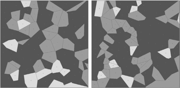
Figure 7.7. Two simulated field patterns (Voronoï diagrams) with random crop rotations

7.5. Architecture

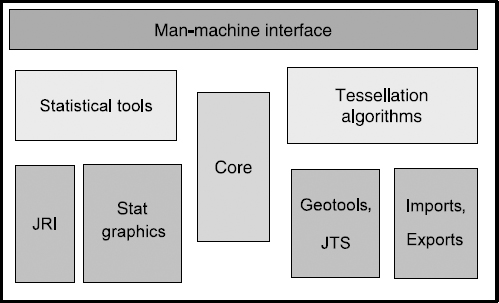
The general architecture is shown in Figure 7.8.

7.5.1. The application Core

This class (see Figure 7.8) contains the list of landscapes thanks to the object LandscapeManager. The latter has all the information to allocate a new identifier to landscapes, and manages the list of landscapes. Thanks to this list, we can run different simulations over a few years. The Core is also the input for R management. It is indeed in this class that the R-Manager is placed, a general class which allows the instancing of classes enabling one to interact with the R application. Here also are usually inserted the inputs toward tessellation and I/O plugins.

Figure 7.8. Architecture

7.5.2. Separating graphical classes from business classes

Graphical displays are handled by a Panel-type object. A LandscapeCreator type object creates a link between the graphics and the landscape. Some mouse functionalities, such as its state as well as its previous state, are externalized into a specific class.

7.5.3. The plugin system

GENEXP-LANDSITES uses a plugin system to represent all the tessellation and landscape I/O algorithms. Its modus operandi is simple. The plugin classes do not need to know their context of use. They are all stored in a class that serves as PluginManager and is integrated in the Core application. The application builds its graphical interface depending on the plugins found when it boots up. For example, the export menu is dynamically created and depends on the loaded export plugins.

7.5.4. Interface

The user is led to successively manipulate different menus according to how he/she wants to use GENEXP-LANDSITES: it can be an exploratory use (for instance, visualizing the different type of landscapes that can be obtained) or a systematic use (generating a set of landscapes from a set of parameters).

The first step is choosing the size of the landscape to be generated, then to outline the zones. Then, for each zone, the user has access to a landscape menu (Figure 7.9) which allows him/her to choose:

• – a seed generation method;
• – a land use distribution;
• – a tessellation method.

Then to access the post-production and embellishment (e.g. choosing the land use colors) and the statistics about each zone in the generated landscape (see Figure 7.10).

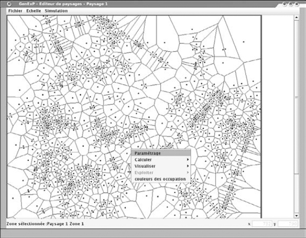
Figure 7.9. GENEXP-LANDSITES interface: landscape menu (one zone, Voronoï tessellation with groups and aligments of seeds)

7.6. Communities

GENEXP-LANDSITES was used for different studies carried out by INRA biologists who were interested in transgene flows [COL 09b, LAV 08] in collaboration with statisticians. Agronomists and other biologsts also expressed interest in this tool and are an active part of the reflection that is currently being carried out on landscape and agricultural land models (see section 7.2)

The contributors are mainly computer science students from degree and master level courses. The different versions of GENEXP-LANDSITES were thus developed during almost 10 successive internships or successive short contracts that took place between 2003 and 2010.

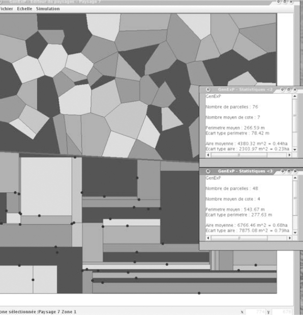
Figure 7.10. GENEXP-LANDSITES interface: landscape menu, statistics (field number, average perimeter and area) display on the different landscape zones (two zones, Voronoï and rectangular tessellation with random seeds)

The main unit holders were at the beginning the LORIA-INRIA Lorraine, a computer science and applications research laboratory⁷ in Lorraine, and the ESE (Environment, Systematics, and Evolution)⁸ laboratory. Today, due to the change in the status of the personnel involved in GENEXP-LANDSITES's development and due to the revamping of various organizations and laboratories, the main unit holders are the INRA, ENGEES⁹, and the INRIA Nancy Grand Est¹⁰.

The development of GENEXP-LANDSITES was funded by the French Research Department (answering the call to tender for “OGM Impact” ), then by the teams' own funds, and more recently by the INRA within the PAYOTE project “Landscape and agricultural land models to study the agro-ecological process” (INRA-INRIA call to tender). These sources of funding did not give us the possibility of contracting an engineer, but a doctoral candidate – working within the INRA-INRIA framework agreement – started his/her dissertation on this topic in October 2010.

7.7. Conclusion

The development of GENEXP-LANDSITES should continue in a wider context. We will notably focus on implementing other tessellation techniques, on simulating other types of seeds (points, segments, and shapes). The spatial analysis possibilities should also be improved to offer users a complete toolbox going from a virtual landscape simulation to their analysis. Finally, we will try to use GENEXP-LANDSITES for new agro-environmental applications to test its use and strengthen the interest it presents.

7.8. Acknowledgments

We would like to thank all the people (researchers and interns involved in the projects “Modeling transgene dissemination at the scale of agricultural landscapes” and “Landscape and agricultural land models to study the agro-ecological process”) who took part in developing GENEXP-LANDSITES since 2003. The original field pattern data were provided for the project by the AUP (Single Payment Agency) and the ipse, the Institute for the Protection and Safety of Citizens (Common Research Center).

7.9. Bibliography

[ADA 07] ADAMCZYK K., ANGEVIN F., COLBACH N., LAVIGNE C., LE BER F., MARI J.-F., “GenExP, un logiciel simulateur de paysages agricoles pour l'étude de la diffusion de transgènes”, Revue Internationale de Géomatique, vol. 17, no. 3-4, pp. 469-487, 2007.

[ANG 02] ANGEVIN F., COLBACH N., MEYNARD J.-M., ROTURIER C., Analysis of necessary adjustements of farming practices, Scenarios for Co-existence of Genetically Modified, Conventional and Organic Crops in European Agriculture, Technical Report Series, EUR 20394 EN, Joint Research Center of the European Commission, 2002.

[ANG 08] ANGEVIN F., KLEIN E.K., CHOIMET C., GAUFFRETEAU A., LAVIGNE C., MESSÉAN A., MEYNARD J.-M., “Modelling impacts of cropping systems and climate on maize cross pollination in agricultural landscapes: the MAPOD model”, European Journal of Agronomy, vol. 28, no. 3, pp. 471–484, 2008.

[AVI 07] AVIRON S., KINDLMANN P., BUREL F., “Conservation of butterfly populations in dynamic landscapes: the role of farming practices and landscape mosaic”, Ecological Modelling, vol. 205, pp. 135–145, 2007.

[BAD 05] BADDELEY A., TURNER R., “Spatstat: an R package for analyzing spatial point patterns”, Journal of Statistical Software, vol. 12, no. 6, pp. 1–42, 2005.

[BOU 10] BOUSSARD H., MARTEL G., VASSEUR C., “Layers dependencies specifications in the APILand simulation approach: an application to the coupling of a farm model and a carabid model”, 2010 International Conference on Integrative Landscape Modelling – LandMod 2010, Poster, Montpellier, France, 2010.

[BRO 09] BROGGI D., GenExp: Génération de paysages agricoles, mémoire de DUT en informatique, IUT Charlemagne, Nancy, June 2009.

[CAR 02] CARSJENS G.J., VAN DER KNAAP W., “Strategic land-use allocation: dealing with spatial relationships and fragmentation of agriculture”, Landscape and Urban Planning, vol. 58, pp. 171–179, 2002.

[CAS 07] CASTELLAZZI M., PERRY J., COLBACH N., MONOD H., ADAMCZYK K., VIAUD V., CONRAD k., “New measures and tests of temporal and spatial pattern of crops in agricultural landscapes”, Agriculture, Ecosystems & Environment, vol. 118, pp. 339–349, 2007.

[CAS 08] CASTELLAZZI M., WOOD G., BURGESS P., MORRIS J., CONRAD K;., PERRY J., “A systematic representation of crop rotations”, Agricultural Systems, vol. 97, pp. 26-33, 2008.

[COL 09a] COLBACH N., “How to model and simulate the effects of cropping systems on population dynamics and gene flow at the landscape level: example of oilseed rape volunteers and their role for co-existence of GM and non-GM crops”, Environmental Sciences and Pollution Research, Springer, Berlin/Heidelberg, vol. 16, no. 3, pp. 348–360, 2009.

[COL 09b] COLBACH N., MONOD H., LAVIGNE C., “A simulation study of the medium-term effects of field patterns on crosspollination rates in oilseed rape (Brassica napus L.)”, Ecological Modelling, vol. 220, no. 5, pp. 662–672, 2009.

[DEL 04] DELAÎTRE J., Simulation de paysages agricoles aléatoires bidimensionnels, mémoire de DUT en informatique, IUT Charlemagne, Nancy, 2004.

[GAR 87] GARDNER R.H., MILNE B.T., TURNER M.G., O'NEILL R.V., “Neutral models for the analysis of broad-scale landscape pattern”, Landscape Ecology, vol. 1, no. 1, pp. 19–28, 1987.

[GAR 91] GARDNER R., O'NEILL R., “Pattern, process, and predictability: the use of neutral models for landscape analysis”, in Quantitative Methods in Landscape Ecology, TURNER M.G., GARONER R.H. (eds), pp. 289–307, Ecological Studies 82, Springer, New York, 1991.

[GAU 06a] GAUCHEREL C., FLEURY D., AUCLAIR D., DREYFUS P., “Neutral models for patchy landscapes”, Ecological Modelling, vol. 197, no. 1–2, pp. 159–170, 2006.

[GAU 06b] GAUCHEREL C., GIBOIRE N., VIAUD V., HOUET T., BAUDRY J., BUREL F., “A domain-specific language for patchy landscape modelling: the Brittany agricultural mosaic as a case study”, Ecological Modelling, vol. 194, no. 1–3, pp. 233–243, 2006.

[GAU 08] GAUCHEREL C., “Neutral models for polygonal landscapes with linear networks”, Ecological Modelling, vol. 219, pp. 39–48, 2008.

[GOT 96] GOTWAY C.A., RUTHERFORD B.M., “The components of geostatistical simulation”, 2nd International Symposium on Spatial Accuracy Assessment in Natural Resources and Environmental Sciences, Fort Collins, USA, 1996.

[GUE 03] GUERREIRO A., Développement d'un générateur expérimental de paysages agricoles aléatoires bidimensionnels, mémoire de DEsS, UHP Nancy 1, 2003.

[HAR 02] HARGROVE W.W., HOFFMAN F.M., SCHWARTZ P.M., “A fractal landscape realizer for generating synthetic maps”, Conservation Ecology, vol. 6, no. 1, pp. 2, 2002. http://www.consecol.org/vol6/iss1/art2/

[KAL 07] KALUZNY L., KOCH O., Pavages du plan dans GenExp, mémoire de projet d'initiation à la recherche, master d'informatique, UHP Nancy 1, May 2007.

[KOS 10] KOSTRZEWA B., Réalisation d'algorithmes numériques pour un logiciel de simulation de cultures, mémoire de DUT en informatique, IUT Charlemagne, Nancy, 2010.

[KUR 00] KURZ W., BEUKAMA S., KLENNER W., GREENOUGH J., ROBINSON D., SHARPE A., WEBB T., “TELSA: the Tool for Exploratory Landscape Scenario Analyses”, Computers and Electronics in Agriculture, vol. 27, pp. 227–242, 2000.

[LAV 08] LAVIGNE C., KLEIN E. K., MARI J.-F., LE BER F., ADAMCZYK K., MONOD H., ANGEVIN F., “How do genetically modified (GM) crops contribute to background levels of GM pollen in an agricultural landscape?”, Journal of Applied Ecology, vol. 45, no. 4, pp. 1104–1113, 2008.

[LAZ 09] LAZRAK E.G., MARI J.-F., BENOÎT M., “Landscape regularity modelling for environmental challenges in agriculture”, Landscape Ecology, Springer, vol. 25, no. 2, pp. 169–183, 1 September 2009.

[LEB 98] LE BER F., BENOIT M., “Modelling the spatial organisation of land use in a farming territory. Example of a village in the Plateau Lorrain”, Agronomie: Agriculture and Environment, vol. 18, pp. 101–113, 1998.

[LEB 06] LE BER F., BENOIT M., SCHOTT C., MARI J.-F., MIGNOLET C., “Studying crop sequences with CARROTAGE, a HMM-based data mining software”, Ecological Modelling, vol. 191, no. 1, pp. 170–185, 2006.

[LEB 09] LE BER F., LAVIGNE C., ADAMCZYK K., ANGEVIN F., COLBACH N., MARI J.-F., MONOD H., “Neutral modelling of agricultural landscapes by tessellation methods – application for gene flow simulation”, Ecological Modelling, vol. 220, pp. 3536–3545, 2009.

[LIU 98] LIU J., ASHTON P. S., “FORMOSAIC: an individual-based spatially explicit model for simulating forest dynamics in landscape mosaics”, Ecological Modelling, vol. 106, pp. 177–200, 1998.

[MAC 96] MACKISACK M., MILES R., “Homogeneous rectangular tessellations”, Advances in Applied Probability, vol. 28, pp. 993–1013, 1996.

[MAR 06] MARI J.-F., LE BER F., “Temporal and spatial data mining with second-order Hidden Markov models”, Soft Computing – A Fusion of Foundations, Methodologies and Applications, vol. 10, no. 5, pp. 406–414, 2006.

[MOR 06] MOREY M., TAYEBI T., Développement d'un logiciel de génération expérimentale de paysages (GenExpNextGen), mémoire de projet d'initiation à la recherche, master d'informatique, UHP Nancy 1, May 2006.

[OKA 00] OKABE A., BOOTS B., SUGIHARA K., NOK CHIU S., Spatial Tessellations: Concepts and Applications of Voronoi Diagrams, 2nd edition, John Wiley & Sons, Chichester, 2000.

[ORO 98] O'ROURKE J., Computational Geometry in C, 2nd edition, Cambridge University Press, Cambridge, 1998.

[SAU 00] SAURA S., MARTÍNEZ-MILLÁN J., “Landscape patterns simulation with a modified random clusters method”, Landscape Ecology, vol. 15, pp. 661–678, 2000.

[SOR 08] SOREL L., Paysages virtuels et analyse de scénarios pour évaluer les impacts environnementaux des systèmes de production agricole, thèse de doctorat, Agrocampus Ouest, Rennes, 2008.

[TUR 91] TURNER M.G., GARDNER R.H., (eds), Quantitative Methods in Landscape Ecology, Ecological Studies 82, Springer, New York, 1991.

[WIT 97] WITH K.A., KING A.W., “The use and misuse of neutral landscape models in ecology”, Oikos, vol. 79, no. 2, pp. 219–229, 1997.