CHAPTER 3

THE PIGEONHOLE PRINCIPLE

The pigeonhole principle is an important key to solving many problems in combinatorics. In this chapter, we discuss several versions of the pigeonhole principle and give many applications.

3.1 The principle

The most important theorem in existential combinatorics is also the simplest: the pigeonhole principle. It occurs in many variations, a few of which we discuss here, and says that not every element in a set is below average and not every element is above average. We now state and prove a general version.

Pigeonhole principle. If f : A → B is a function, with A and B finite nonempty sets, then the following two statements hold:

(1) ‘There exists b B with |f⁻¹ (b)| ≥ |A|/|B|.

(2) There exists b B with |f⁻¹ (b)| ≤ |A|/|B|.

Proof. We prove (1) by contradiction. Suppose that |f⁻¹ (b)| < |A|/|B| for all b B. Then

We conclude that |A| < |A|, an absurdity. Therefore, our assumption that |f⁻¹ (b)| < |A|/|B| for all b B is false. Hence, there exists b B with |f⁻¹ (b)| ≥ |A|/|B| for all.

We prove (2) by replacing “<” by “>” in the above argument.

EXAMPLE 3.1 Sets of cards

Solution: Let the three suits be designated by C, H, and S. If the five cards do not include one card of each suit, then at least one suit is absent, say S. Therefore, we may define a function f: {a, b, c, d, e} → {C, H} from the five cards to their respective suits. (The function isn’t necessarily onto.) By the pigeonhole principle, the preimage of one suit contains at least three cards. These cards constitute a set.

Proof. (1) If the inequality holds for no i, then

a contradiction.

If |A| = |B| + 1, then the following special case of the pigeonhole principle results.

This version of the pigeonhole principle is often paraphrased as: “If n + 1 objects are placed in n pigeonholes, then at least one pigeonhole must contain at least two objects.” Hence the term pigeonhole principle.

We now give a pigeonhole principle proof of a very old but interesting result in number theory. For different proofs, see [21].

Proof. Define by letting f(j) be the subinterval of [0, 1) which contains jα — [jα]. (Note that [x] is the greatest integer less than or equal to x.) The pigeonhole principle implies the existence of j, k(j > k) with f(j) = f(k). According to the definition of the function f, there exists a positive integer p with |jα – kα – p| < 1/n. Letting q = j – k (so that 1 ≤ q ≤ n), the inequality becomes |α – p/q| < 1/qn ≤ 1/q².

This theorem is used to ensure good rational approximations to irrational numbers α. For example, taking α = π and n = 10, the theorem guarantees the existence of a rational number p/q with |π – p/q| < 1/10q ≤ 1/q². In fact, the well-known approximation 22/7 satisfies the inequality. Can you find an approximation to α = with n = 10?

In the preceding versions of the pigeonhole principle we have assumed that both the domain and the codomain are finite sets. If the domain is infinite, then the following highly useful infinitary pigeonhole principle results.

EXERCISES

3.1 Using the pigeonhole principle, show that some positive integral power of 17 ends in 0001 (base 10).

3.2 Let q be an odd integer greater than 1. Show that there is a positive integer n such that 2ⁿ – 1 is a multiple of q.

3.3 Let A₁,…,A₁₀₀ be subsets of a finite set S, each with |A_i| > |S|. Prove that there exists x S with x contained in at least 67 of the A_i. Show that 67 is the best possible result.

3.4 Prove that if S is a subset of {1,…,2n} and |S| > n, then there exist x, y S with x and y relatively prime.

3.5 Prove that if S is a subset of {1,…,2n} and |S| > n, then there exist x, y S with x a divisor of y.

3.6 (Putnam Competition, 1964) Let S be a set of n > 0 elements, and let A₁, A₂,…,A_k be a family of distinct subsets, with the property that any two of these subsets meet. Assume that no other subset of S meets all of the A_i. Prove that k = 2ⁿ⁻¹.

This result is generalized in many interesting ways in [3].

3.7 Prove the infinitary pigeonhole principle.

Hint: Assume that f⁻¹(b) is finite for all b B and obtain a contradiction.

3.8 Prove that every polyhedron has two faces with the same number of edges.

3.9 Let A be an m × n matrix with distinct real number entries in increasing order in each row from left to right. Rearrange the elements of each column of A so that they are in increasing order from top to bottom; call the resulting matrix A′. Show that the elements of each row of A′ are in increasing order from left to right.

3.10 An n × n binary matrix contains a 1 in every row, column, and diagonal (diagonals of every length are considered here). What is the minimum number of 1′s in this matrix?

3.11 Let L₁ be a two-row array of positive integers

where the a_i are distinct integers written in increasing order. Let c₁,…,c_n (c₁ ≤ c₂ ≤ · · · c_n) be the list of all integers that occur in L₁, and for 1 ≤ i ≤ m, let d_i be the number of occurrences of c_i in L₁. Let L₂ be the array

For example, if L₁ is the array

then L₂ is the array

Starting with any array L₁, the array L₂ is created as indicated above. Then the operation is repeated on L₂ to form a new array L₃, and so on. Show that the number of distinct arrays produced in this manner is always finite. We say that each sequence of arrays eventually “goes into a loop.” Show that a loop always consists of one, two, or three arrays.

3.2 The lattice point problem and SET^®

In this section, we apply the pigeonhole principle to problems concerning lattice points in Euclidean space.

A lattice point in the plane is an ordered pair p = (x, y) with integer coordinates x and y.

EXAMPLE 3.2 A lattice point midpoint

Solution: Define a function

by mapping p_i to the ordered pair (x_i mod 2, y_i mod 2). By the pigeonhole principle, some two points p_i and p_i have the same image. These points satisfy the requirement of the problem, for the midpoint of p_ip_j is ((x_i + x_j)/2, (y_i + y_j)/2). Both coordinates are integers because x_i, x_j have the same parity and y_i, y_j have the same parity.

The “five” in the problem above is best possible in the sense that one can find four lattice points determining no lattice midpoint, e.g., (0, 0), (0, 1), (1, 0), (1, 1).

EXAMPLE 3.3 A lattice point centroid

Solution: We show that n ≤ 13 by defining a function f: {p₁,…,p₁₃} → {0, 1, 2} which maps p_i to the residue class modulo 3 of its first coordinate. By the pigeonhole principle, some five lattice points, say p₁, p₂, p₃, p₄, p₅, have the same image. By the analysis of the suits in the board game mentioned in Example 3.1, some three of these points, say p₁, p₂, p₃, have second coordinate residues 000, 111, 222, or 012. These three lattice points determine a lattice point centroid. Therefore, n exists and satisfies n ≤ 13.

The determination of the minimum n that forces the existence of three points determining a lattice point centroid is a more difficult matter. It turns out that the minimum value is n = 9. The argument is carried out modulo 3. Thus, there are just nine possible ordered pairs from which to choose. The following list of ordered pairs (modulo 3) shows that n > 8:

In order to prove n ≤ 9, we must show that any nine points include three whose first coordinates and second coordinates are of the form 000, 111, 222, or 012. The nine possible ordered pairs are conveniently represented by the nine non-ideal points of the order 3 projective plane of Figure 6.1. The 12 lines of the figure (excluding the line at infinity) correspond to triples of points which determine a lattice point centroid. If any ordered pair is chosen three times, these three ordered pairs determine a lattice point centroid. Therefore, let us assume that each ordered pair is chosen at most twice, and hence at least five different ordered pairs are chosen. By shuffling the rows and columns of the figure (if necessary), we may assume that three of the points are (0, 0), (1, 0), and (1, 1). If no three points are collinear, then we may not choose the points (2, 0), (0, 2), or (2, 2). This means that we must choose two of the three points (1, 1), (2, 1), and (1, 2). But any of these choices gives three collinear points: (0, 1), (1, 1), and (2, 1); (1, 0), (1, 1), and (2, 1); or (0, 0), (1, 2), and (2, 1).

The d-dimensional generalization of the above problem calls for the minimum n such that, given any n lattice points in R^d (ordered d-tuples of integers), some k determine a lattice point centroid. Let n(k, d) be the minimum such n. The existence of n(k, d) is guaranteed by the pigeonhole principle, and, in fact, the pigeonhole principle yields an upper bound for n(k, d) on the order of k^d+1. The set of d-tuples each of whose coordinates is 0 or 1, taken with multiplicity k – 1, establishes the lower bound n(k, d) > (k – 1)2^d.

This question is known as the lattice point problem. Trivially, n(1, d) = 1. In 1961 Paul Erds, A. Ginzburg, and A. Ziv proved that n(k,1) = 2k – 1. It has since been shown that n(3, 3) = 19; she Problem 6298, American Mathematical Monthly 89 (1982) 279–280. In 2003 Christian Reiher and Carlos di Fiore proved that n(k, 2) = 4k – 3. An exercise calls for a proof that n(2, d) = 2^d + 1.

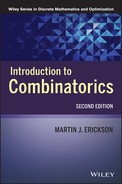
A situation similar to the lattice point problem comes from a card game called SET®, created by the population geneticist Marsha Falco. The game is played with cards identified by four attributes: number, shape, color, and shading. Each attribute occurs with three possible values (e.g., shape = oval, diamond, or squiggle). Hence there are 81 cards. Thinking of the attributes as coordinates and the values as residue classes, the cards are represented as 4-tuples over Z₃, e.g., (0, 1, 0, 1), (2, 1, 0, 2), and (1, 1, 1, 1). A “set” consists of three cards that, with respect to each attribute, all agree or all disagree. For example, the cards corresponding to (0, 1, 1, 2), (0, 2, 0, 2), and (0, 0, 2, 2) constitute a set. The game is similar to the lattice point problem with k = 3 and d = 4, but in the game no 4-tuple of coordinates is repeated. One can define a generalized version of the game in which there are d attributes each occurring with k possible values. Hence, there are k^d cards. A set consists of k cards that all agree or all disagree on each attribute. Equivalently, a card is a vector with d coordinates, each of which can take k values. A set is a collection of k vectors, which in each coordinate all agree or all disagree. Then we can define the generalized SET® function n′(k, d) to be the minimum number of cards (or vectors) that guarantee a set. Little is known about the function n′(k, d). The values n′(3, 4) = 21, n′ (3, 5) = 46, and n′(3, 6) = 113 are known. A collection of 20 cards containing no set is shown in Figure 3.1 (the four-dimensional space is represented by a three-by-three array of three-by-three arrays). Information on SET may be found at http://www.setgame.com.

Figure 3.1 Twenty cards containing no set.

The functions n(k, d) and n′(k,d) are similar, although there are two differences. A minor difference is that in the card game each d-tuple occurs exactly once while in the lattice point problem repetition is allowed. A more important difference is that in the lattice point problem we require that a sum of lattice points be zero modulo k, while in the card game we require that the cards all agree or all disagree in each coordinate. For example, the lattice points (1, 0), (1, 1), (3, 0), and (3, 3) have a lattice point centroid, but the corresponding cards do not constitute a set (with k = 4). If k = 3, this difference disappears.

We mentioned that the value n(3, 3) = 19 has been proved. The corresponding fact in the card game is that n′(3, 3) = 10.

In the card game setting, there are 27 possible cards (each defined by three attributes that occur with three possible values). We would like to show that every collection of 10 cards contains a set. To translate back to the lattice point problem, assume that we have 19 ordered triples of numbers modulo 3. If no triple is repeated three times, then, by the pigeonhole principle, there must be at least 10 distinct triples. An exercise calls for a construction to show that n(3, 3) > 18 (and incidentally n′(3, 3) > 9).

It is convenient to represent the cards both as integers between 0 and 26 (inclusive) and as 3-tuples of elements in Z₃. We define these 3-tuples as the base 3 digits of the numbers.

The number of 10-subsets of a 27-element set is = 8,436,285, and this is too many subsets to test. We will discuss a way to reduce the number of 10-subsets which must be examined.

Without loss of generality, we may assume that 0 (0, 0, 0) is an element of each 10-subset. Also, we note that in any 10-subset of Z³₃ there exist three linearly independent vectors (a plane contains only nine points). By a linear transformation (a 3 × 3 matrix), we may map these three vectors to the specific vectors 1 (0, 0, 1), 3 (0, 1, 0), and 9 (1, 0, 0). Therefore, since linear transformations map sets to sets, we need only consider 10-subsets that contain these three points. Furthermore, each pair of the four points 0, 1, 3, 9 determines a third point which forms a set with that pair. There are 6 such points, namely, 2 (0, 0, 1), 6 (0, 2, 0), 18 (2, 0, 0), 8 (0, 2, 2), 20 (2, 0, 2), and 24 (2, 2, 0). If any of these points is present in a 10-subset, then the 10-subset contains a set and we do not need to examine it. We can therefore exclude these six points from consideration.

To summarize, of the integers 0 through 26 (inclusive), the integers 0, 1, 3, and 9 are included in every 10-subset, and the integers 2, 6, 8, 18, 20, and 24 are excluded in every 10-subset. Hence, we now have only = 12,376 subsets to examine.

A computer run can check these subsets and thereby show that every 10-subset contains a set, and therefore n′(3, 3) = 10 and n(3, 3) = 19.

EXERCISES

3.3 Graphs

Graph theory began in 1736 when Leonhard Euler (1707–1783) solved the famous concerning a certain system of seven bridges over the river Pregel. See [16]. In the last 50 years there has been an explosion in graph theory research and applications. Today, there are many areas of graph theory research including algebraic graph theory, extremal graph theory, and topological graph theory. Within combinatorics, graph theory is closely related to design theory, Ramsey theory, and coding theory. In this section we give some basic definitions and an indication of the deeper results of graph theory which will be studied in the next chapter.

A graph G is an ordered pair (V, E), consisting of a vertex set V and an edge set E [V]². Vertices are also called points or nodes. Edges are also called lines or arcs. In our definition of graph there are no loops or multiple edges. In a drawing of a graph, two vertices x and y are joined by a line if and only if {x, y} E. Two vertices joined by a line are said to be adjacent; if they are not joined by a line, they are nonadjacent. If |V| = p and |E| = q, then we say that G has order p and size q. The degree of a vertex v, denoted δ(v), is the number of edges incident to v. The complement of a graph G has the same vertex set as G, but two vertices are adjacent in if and only if they are nonadjacent in G.

Certain graphs occur so frequently that they require names. The complete graph K_n, consists of n vertices and all possible edges. The complete bipartite graph K_{m, n} consists of a set A of m points, a set B of n points, and all the mn edges between A and B. The infinite complete graph K_∞ contains a countably infinite set of points and all possible edges. Likewise, the infinite complete bipartite graph K_{∞, ∞} contains countably infinite sets A and B and all edges between A and B. The cycle C_n consists of n vertices connected by n edges in a cyclical fashion. The path P_n is C_n minus an edge. Figure 3.2 illustrates some of these graphs. For general references on graph theory, see [13], [5], and [28].

Figure 3.2 A complete graph, a complete bipartite graph, a cycle, and a path.

One of the most elementary propositions of graph theory is called the “Handshake Theorem.” If some people in a group shake hands, then there will be two people who shake the same number of hands.

Proof. Suppose that G has p vertices. Then each vertex has degree equal to one of the numbers 0,…,p – 1. However, it is impossible for G to have both a vertex of degree 0 and a vertex of degree p – 1. Therefore the list of degrees of the p vertices contains at most p – 1 different numbers. By the pigeonhole principle, some two vertices have the same degree.

If δ(v) is the same for all vertices, then we say that G is regular of degree δ(v). Note that complete graphs and cycles are regular.

If G is any finite graph, the independence number α(G) is the maximum possible number of pairwise nonadjacent vertices of G. The chromatic number χ(G) is the minimum number of colors in a coloring of the vertices of G with the property that no two adjacent vertices share the same color.

Here is another simple theorem proved by the pigeonhole principle.

Proof. Consider the vertices of G as partitioned into χ(G) color classes. By the pigeonhole principle, one of the classes must contain at least p/χ(G) vertices, and these vertices are pairwise nonadjacent. Thus α(G) ≥ p/χ(G) and the result follows immediately.

Equality in the above theorem holds, for example, when G consists of the vertices and edges of a cube.

The famous “four color theorem,” proved in 1976 by Kenneth Appel and Wolfgang Haken, is the statement that χ(G) ≤ 4 for any planar graph G. (A graph is planar if it can be drawn in the plane without edge crossings.) Combining this result with the theorem on the independence number and chromatic number of a graph, we arrive at the relation α(G) ≥ p/4 for any planar graph G. We can turn a planar graph into a planar map by placing a territory at each vertex and allowing two territories to share a common boundary when the two vertices in the graph are adjacent. In terms of maps, Appel and Haken’s result is that every map can be colored with four colors so that no two bordering territories have the same color. It follows from the theorem on the independence number and chromatic number of a graph that any planar map on p vertices contains at least p/4 territories no two of which share a border.

A path in a graph G from vertex v₀ to vertex v_n is a sequence of distinct edges

The path is simple if the vertices v₁, v₂,…,v_n are distinct. A circuit is a path from v to v for some vertex v. A simple circuit is a cycle. We say that G is connected if there is a path between every two vertices. Note that each of the graphs in Figure 3.2 is connected.

The next result, a special case of Turán’s theorem called Mantel’s theorem, foreshadows Ramsey’s theorem of the next chapter.

We consider an extremal property of graphs. How many edges are possible in a triangle-free graph G on 2n vertices? Certainly, G can have n² edges without containing a triangle: let G be the complete bipartite graph K_n,n, consisting of two sets of n vertices each and all the edges between the two sets. Indeed, n² turns out to be the maximum possible number of edges. That is, if G has n² + 1 edges, then G contains a triangle. This we prove by mathematical induction using the pigeonhole principle.

Proof If n = 1, then G cannot have n² + 1 edges; hence the statement is vacuously true. Assuming the result for n, we now consider a graph G on 2(n + 1) vertices with (n + 1)² + 1 edges. Let x and y be adjacent vertices in G, and let H be the restriction of G to the other 2n vertices. If H has more than n² edges, then we are finished by the induction hypothesis. Suppose that H has at most n² edges, and therefore at least 2n + 1 edges join x and y to vertices in H. By the pigeonhole principle, there exists a vertex z in H that is adjacent to both x and y. Hence G contains the triangle xyz.

Proof. The argument uses induction on n and the previous theorem. For n = 1, the result is trivially true. Assume the result holds for n. Let G be a graph on 2(n + 1) vertices with (n + 1)² edges and no triangle. Let u and v be connected vertices in G. Let H be the graph restricted to the other 2n vertices. By the previous theorem, H has at most n² edges. However, if H has less than n² edges, then there are more than 2n edges between the set {u, v} and H; by the pigeonhole principles, there exists a triangle. Hence, H has exactly n² edges, H is isomorphic to K_n,n, and there are exactly 2n edges from {u, v} to H. The reader can now show that u and v are each joined by n edges to H, with u joined to one independent set in H and v joined to the other. Therefore, G is isomorphic to K_n+1,n+1. This completes the induction and the proof.

EXERCISES

3.4 Colorings of the plane

The concept of this section, partitions of the plane, foreshadows Van der Waerden’s theorem of Chapter 4.

Suppose that the plane is partitioned into two (disjoint) subsets G and R (green and red). We will show that one of the two subsets contains the vertices of a Euclidean rectangle with sides parallel to the coordinate axes. In fact, partitioning the whole plane is unnecessary. The same result follows if we partition just the 21 lattice points of N₇ × N₃ into two subsets, so let us assume only that. We say that each lattice point is “colored” either G or R.

Proof. Each column of three points in this lattice contains three points of color G, two G′s and one R, two R′s and one G, or three R′s. For the moment, the relevant fact is that there is a majority of G′s or a majority of R′s in each column. Let us refer to a column as a G-majority or an R-majority column. By the pigeonhole principle, some four columns are G-majority or some four columns are R-majority. Without loss of generality, suppose that there are four G-majority columns. We will show that there are four points all colored G which are the vertices of a rectangle. If any of the four G-majority columns contain three points colored G, then we handicap ourselves by changing the color of an arbitrary point to R. (Our result will follow even with this handicap.) Now we have four columns which each contain exactly two points colored G and one point colored R. There are three possible patterns for the configuration of the points: GGR, GRG, and RGG. By the pigeonhole principle, there are two columns with the same color pattern. The four G′s in these columns are the vertices of a rectangle with sides parallel to the coordinate axes.

It is easy to see that neither the lattice N₇ × N₂ nor the lattice N₆ × N₃ is sufficient, when 2-colored, to force the existence of four monochromatic points on the vertices of a rectangle with sides parallel to the coordinate axe’s. Thus, the lattice N₇ × N₃ is minimal with respect to this property.

EXERCISES

3.5 Sequences and partial orders

Every sequence of 10 distinct integers contains an increasing subsequence of four integers or a decreasing subsequence of four integers (or both). For example, the sequence 5, 8, –1, 0, 2, –4, –2, 1, 7, 6 contains the increasing subsequence –1, 0, 2, 7.

This proposition is an existence result. No matter which 10 integers are chosen, and no matter in what order they occur, there exists a specific type of subsequence, namely, a monotonic subsequence of four integers.

In this section, we apply the pigeonhole principle to two types of mathematical structures: sequences and partial orders. Our goal is to show that arbitrary sequences and partial orders contain highly nonrandom substructures. This is indicative of a basic principle of existential combinatorics: complete disorder is impossible.

A sequence (finite or infinite) is increasing (or strictly increasing) if a_i < a_i for all i < j; decreasing (or strictly decreasing) if a_j > a_j for all i < j; monotonically increasing if a_i ≤ a_j for all i < j; monotonically decreasing if a_i ≥ a_j for all i < j; and monotonic if it is either monotonically increasing or monotonically decreasing.

EXAMPLE 3.4

We say that {b₁,…,b_m} is a subsequence of {a₁,…,a_n} if there exists a strictly increasing function f : {1,…,m} → {1,…,n} for which b_i = a_f(i) for all i.

EXAMPLE 3.5

Proof. Suppose that S = {a₁,…,a_mn+1} is a sequence of real numbers. For 1 ≤ k ≤ mn + 1, let i_k be the length of a longest monotonically increasing subsequence starting with a_k, and let d_k be the length of a longest monotonically decreasing subsequence starting with a_k. Then the ordered pairs (i_k, d_k) are distinct. For if j < k and a_j ≤ a_k, then i_j > i_k, while if j < k and a_j ≥ a_k, then d_j > d_k. But by the pigeonhole principle, if 1 ≤ i_k ≤ m and 1 ≤ d_k ≤ n, for all k, then some ordered pairs (i_k, d_k) are not distinct. Therefore, i_k ≥ m + 1 or d_k ≥ n + 1 for some k.

EXAMPLE 3.6

The expression mn + 1 in the Erds—Szekeres theorem is best possible in the sense that there exists a sequence of mn real numbers which contains neither a monotonically increasing subsequence of m + 1 terms or a monotonically decreasing subsequence of n + 1 terms. We form such a sequence by concatenating n sequences of m increasing terms in the following manner. For each j N_n, let S_j =– {a_1j,…,a_mj} be an increasing sequence of m real numbers, and suppose that every term of S_j is greater than every term of S_k whenever j < k. Then the sequence

contains no increasing subsequence of length m + 1 and no decreasing subsequence of length n + 1. In general, there are many sequences which avoid monotonic subsequences of these lengths. The question of the number of such sequences is answered by the theory of Young tableaux. See Notes.

Proof. Let S = {a₁, a₂,…} be an arbitrary infinite sequence of real numbers. We will inductively define an infinite monotonic subsequence of S. Relabel the elements of S as {a₁₁, a₁₂,…}. By the infinitary pigeonhole principle, there exists an infinite subsequence S₂ = {a₂₂, a₂₃,…} of S– {a₁₁} all of whose elements are greater than or equal to a₁₁ or all of whose elements are less than or equal to a₁₁. Continuing in this manner, we find an infinite subsequence S₃ = {a₃₃, a₃₄, a₃₅,…} of S₂ – {a₂₂} all of whose elements are greater than or equal to a₂₂ or all of whose elements are less than or equal to a₂₂. This process continues, defining a new subsequence S_i at each step. The subsequence T = {a₁₁,a₂₂, a₃₃,…} has the property that each element a_ii is greater than or equal to all elements following it, or less than or equal to all elements following it. Again, by the infinitary pigeonhole principle, there exists a subsequence U of T each of whose elements is greater than or equal to those following it or each of whose elements is less than or equal to those following it. Thus, U is an infinite monotonic subsequence of S.

The set of real numbers R is linearly ordered. For any two distinct real numbers x and y, either x < y or y < x. The forthcoming Dilworth’s lemma generalizes the Erdős–Szekeres theorem to partially ordered sets.

Recall that a partial order on X is a relation on X that is reflexive, antisymmetric, and transitive. We often denote a partial order by and write a b when (a, b) . Two elements a, b X are comparable if a b or b a and incomparable otherwise. For example, the relation a b if and only if a divides b is a partial order on N.

A partial order on X is a total order (or linear order) if every two elements of X are comparable. For example, the usual ≤ relation is a linear order on N. If is a partial order on X, and Y is a subset of X in which every two elements are comparable, then Y is a chain. If no two distinct elements of Y are comparable, then Y is an antichain. The length of a partially ordered set X is the greatest number of elements in a chain of X, and the width is the greatest number of elements in an antichain.

EXAMPLE 3.7

Figure 3.3 is the directed graph representation of the partial order

Figure 3.3 A partial order of width 3 and length 3.

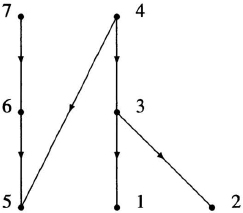
on the set X = {1, 2, 3, 4, 5, 6, 7}. The arrows required for reflexivity and transitivity are suppressed in the diagram. The length and width of are both 3. For instance, {1, 3, 4} is a chain of length 3 and {1, 2, 6} is an antichain of size 3.

The length and width of a partial order are related to the size of the underlying set by the following result of R. P. Dilworth.

Proof. Let X be an arbitrary partially ordered set with mn + 1 elements. Suppose that X contains no chain of size m + 1. Then we may define a function f : X → {1,…,m} with f (x) equal to the greatest number of elements in a chain with greatest element x. By the pigeonhole principle, some n + 1 elements of X have the same image under f. By the definition of f, these elements are incomparable; they form an antichain of size n + 1.

EXAMPLE 3.8

Notice the similarity between Dilworth’s lemma and the Erdős–Szekeres theorem. In each case, the hypothesis concerns a set of mn + 1 elements and the conclusion concerns subsets of sizes m + 1 and n + 1. These similarities are no coincidence. In fact, the Erdős–Szekeres theorem may be proved as a corollary of Dilworth’s lemma. Let S = {a₁,…,a_mn+1} be a sequence of mn + 1 real numbers. Define a partial order on S by setting a_i a_j if a_i ≤ a_j and i ≤ j. Dilworth’s lemma guarantees a chain of m+1 elements (corresponding to a monotonically increasing subsequence of m + 1 terms) or an antichain of n + 1 elements (corresponding to a monotonically decreasing subsequence of n + 1 terms).

Just as the Erdős–Szekeres theorem is a best possible result, so also is Dilworth’s lemma. In the exercises, the reader is asked to furnish an example of a partial order on mn elements with length m and width n.

Dilworth’s lemma is sometimes easier to apply in the following form.

Proof. Suppose, to the contrary, that n > lw + 1. Then, by DilWorth’s lemma, there is a chain of length l + 1 or an antichain of size w + 1; these results contradict the definition of l or w.

As you probably suspect, there is an infinitary version of Dilworth’s lemma. The proof is an exercise.

The title Dilworth’s lemma suggests that there might be a Dilworth’s theorem, which is the case.

Proof We only prove that X can be partitioned into l antichains. For a proof that X can be partitioned into w chains, see [4] or [5].

Define f : X → {1,…,l} by letting f(x) be the maximum number of elements in a chain with greatest element x. The preimage of each y {1,…,l} is an antichain.

EXAMPLE 3.9

EXERCISES

3.32 Let n² + 1 distinct points be given in R². Prove that there is a sequence of n + 1 points (x₁, y₁),…,(x_n+1, y_n+1) for which x₁ ≤ x₂ ≤ · · · ≤ x_n+1 and y₁ ≥ y₂ ≥ · · · ≥ y_n+1 or a sequence of n + 1 points for which x₁ ≤ x₂ ≤ · · · ≤ x_n+1 and y₁ ≤ y₂ ≤ · · · ≤ y_n+1.

3.33 Give an example of a partial order on mn elements with length m and width n.

3.34 (Putnam Competition, 1967) Let 0 < a₁ < a₂ < · · · < a_mn+1 be mn + 1 integers. Prove that you can select either m + 1 of them no one of which divides any other, or n + 1 of them each dividing the following one.

Hint: Apply Dilworth’s lemma.

3.35 For any n²+1 closed intervals of R, prove that n + 1 of the intervals share a point or n + 1 of the intervals are disjoint.

Hint: Let α β if the closed interval α is entirely to the left of the closed interval β. Apply Dilworth’s lemma.

3.36 Prove the infinitary Dilworth’s lemma.

3.37 Prove the infinitary Erdős–Szekeres theorem as a corollary of the infinitary Dilworth’s lemma.

3.38 Let ₁ and ₂ be two total orders on a set of size n² + 1. Show that there is a subset of size n + 1 on which ₁ and ₂ totally agree or totally disagree.

3.39 Prove that if 2n – 1 total orders are given on m²²ⁿ⁻² + 1 points, then some m + 1 points are totally ordered by n agreeing orders.

3.6 Subsets

Let X(t) be the collection of subsets of the t-element set N_t, and let be the containment partial order on X(t). For instance, if t = 3, then X(t) consists of eight elements: θ, {1}, {2}, {3}, {1,2}, {1,3}, {2,3}, and {1,2,3}. Some examples of containment are {1, 2} {1, 2, 3}, θ {3}, and {1, 3} {1, 3}. The size of X(t) is 2^t. What are the length and width of ? The length is t + 1, because the longest chains start with θ and include one new element at each step until all t elements are included. The width of is the subject of Sperner’s theorem. Remember that an antichain of X(t) is a collection of subsets of N_t none of which contains another.

Emanuel Sperner (1905–1980) proved the following result in 1928. We give a simpler proof essentially due to D. Lubell. See [9]. For a proof of Sperner’s theorem using the probabilistic method, see [2].

Note that Sperner’s theorem tells us that the width of the partially ordered set X(t) is .

Proof Let A = {A₁,…,A_m} be an antichain of subsets of N_t with |A_i| = α_i at for 1 ≤ i ≤ m. For each i, the set A_i is contained in exactly α_i!(t – α_i)! chains of length t + 1. (Such chains commence with the empty set, add one element at a time until A_i is exhausted, then add one element at a time until the complement of A_i is exhausted.) Because these chains are distinct and there are t! chains of length t + 1 altogether,

Dividing this inequality by t! we obtain

Since (^t_k) is maximized when k = [t/2], it follows that

Therefore

What are the antichains of X (t) with elements? Equality in the above relation can be attained only if for each α_i. If t is even, this forces α_i = t/2. If t is odd, then α_i can equal (t – 1)/2 or (t + 1)/2. We now prove that if t is odd, then all elements of the antichain are size (t – 1)/2 or all are size (t + 1)/2. The proof is essentially due to Lásló Lovász.

Proof. We have already demonstrated the t even case. Suppose that t = 2u + 1. As each maximal chain in X(t) contains exactly one element of A, if U is a subset of size u, V is a subset of size u + 1, and U V, then A contains exactly one of U and V. Suppose that U is a subset of size u contained in A, and U’ is any other subset of size u. Then there is a sequence of subsets

beginning with U and ending with U’, whose sizes alternate between u and u + 1, and such that V_i contains U_i, and U_i+1 for each i. It follows that U’ is an element of A. Because U’ was arbitrary, A contains all subsets of size u. A similar argument shows that if A contains at least one subset of size u + 1, then A contains every subset of size u + 1.

We are now ready to look at relations which are not transitive. In Chapter 4 we begin by discussing graphs, where the relations are merely reflexive and symmetric. The theorems are more difficult to prove in this more general setting—and the analysis of best possible results is much more difficult.

EXERCISES

3.40 Let a₁,…,a_n, b R, with all a_i ≥ 1. Show that the maximum number of sums ±a₁ ± a₂ ± · · · ± a_n in the open interval (b, b + 2) is .

3.41 Let a₁,…,a_n be positive real numbers. Show that the maximum number of equal sums ₁a₁ + · · · + _na_n (_i = 0 or 1) is .

See [3] and [26] for a discussion of the Littlewood–Offord problem concerning the number of sums Σⁿ_{i=1 i}z_i (_i = ±1 and |z_i| ≥ 1) lying inside any given circle in the complex plane.

Notes

Johann Peter Gustav Lejeune Dirichlet (1805–1859) was the first mathematician to explicitly use the pigeonhole principle in proofs. He referred to it as the “drawer principle.”

The word “graph” was first used in mathematics in an 1877 paper by James Sylvester (1814–1897). In 1936 Dénes König (1884–1944)> wrote the first book on graph theory, Theorie der endlichen and unendlichen Graphen.

The special case of Turán’s theorem (1941) was proved by W. Mantel in 1907.

The Erds–Szekeres theorem was proved in 1935 and may be regarded as a sort of proto-Ramsey theorem (even though Ramsey’s theorem was proved in 1930).

According to the Erds–Szekeres theorem, every permutation of the numbers 1,…,10 contains a monotonic subsequence of length four. But this result does not hold for permutations of the numbers 1,…,9; there are many permutations of 1,…,9 that do not have a monotonic subsequence of length four. The question of exactly how many is answered by the theory of Young tableaux. For a discussion of Young tableaux, see [19] and [26]. We give a few details here.

Let n = λ₁ + · · · + λ_n. A Young tableau of shape λ₁ + · · · + λ_n is a Ferrers diagram of shape (λ₁,…,λ_n) in which each dot has been replaced by a different integer from the set {1,…,n}. The number n is the order of the tableau. The positions in a tableau are called cells. A standard tableau is one in which the integers increase in every column and in every row.

Figure 3.4 shows an example of a standard Young tableau with n = 9 = 4+3+2.

Figure 3.4 A standard Young tableau of shape 4 + 3 + 2.

How many standard Young tableaux have this shape? The answer is given by the hook-length formula. We define the hook-length of a cell to be one more than the number of cells to its right and below it. Figure 3.5 shows the hook-lengths of the cells of the tableau of Figure 3.4.

Figure 3.5 The hook-lengths of the cells of a tableau.

The hook-length formula says that the number of standard Young tableaux of a given shape is equal to n! divided by the product of the hook-lengths. Thus, the number of standard Young tableaux of shape 4 + 3 + 2 is

There are 30 partitions of the number 9. For each such partition λ, let f_λ be the number of standard tableaux of shape λ. If you compute these numbers (via the hook-length formula), you may be surprised to find that

This identity (for any positive integer n) is known as Schur’s formula. It is used in the theory of representations of the symmetric group.

Schur’s formula indicates that there is a correspondence between pairs of standard Young tableaux of identical shape and permutations of n. This correspondence is effected by the Robinson–Schensted algorithm.

We give an example of the algorithm. Let n = 9 and

We will construct an ordered pair (P, Q) of standard Young tableaux (of the same shape) corresponding to σ.

The first task is to construct P. (We will construct Q later.) We read the permutation σ from left to right and construct P step by step. The 5 is placed in the top left position of the tableau, and the 8, being greater than 5, is placed below:

Now we come to the 3. Being less than 5, the 3 “bumps” the 5 to the right and takes its place:

Likewise, 2 is less than 3, so it bumps the 3 to the right (arid the 5 along with it) and takes its place:

Now comes the 7. Because 7 is less than 8, it is inserted into the second row, bumping the 8 to the right. Then the 6 bumps the 7 (and the 8 along with it):

Next, the 4 bumps the entire second row to the right, and the 8 is bumped up to the first row:

Finally, the 9, being greater than 4, is placed in the third row, and the 1 bumps the first row to the right:

This completes the tableau P. The tableau Q consists of the numbers 1,…,9 in a tableau of the same shape as P and in the order in which new positions were occupied in P. Figure 3.6 shows P and Q.

Figure 3.6 The tableaux P and Q corresponding to σ = 583276491.

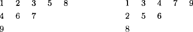
In the Robinson–Schensted correspondence, the number of columns of the tableaux P and Q is equal to the length of a longest decreasing subsequence of the permutation, and the number of rows is equal to the length of a longest increasing subsequence. In our example, the tableaux have five columns and three rows, and indeed, a longest decreasing subsequence of σ has five terms and a longest increasing subsequence has three terms.

To calculate the number of permutations of {1,…,9} with no monotonic subsequence of length four, we use the hook-length formula to find the number of standard Young tableaux of shape 3 + 3 + 3:

Since the desired permutations correspond to ordered pairs of standard Young tableaux of this shape, the number of such permutations is 42² = 1764.

We leave five problems for you to ponder:

1. How does the reverse direction of the Robinson–Schensted algorithm work?

2. In the Robinson–Schensted correspondence, show that the number of columns of the tableaux P and Q is equal to the length of the longest decreasing subsequence of σ. Show that the number of rows is equal to the length of the longest increasing subsequence of σ.

3. If the permutation σ corresponds to the pair of tableaux (P, Q), show that σ⁻¹ corresponds to the pair (P, Q).

4. A permutation σ S_n is called an involution if σ = σ⁻¹. Show that the number of involutions in S_n, equals the number of standard tableaux of order n. Recall that these were counted in Exercise 2.69.

5. Show that the number of standard Young tableaux of shape 2 × n is given by the Catalan number C_n.