CHAPTER 2
GENERATING FUNCTIONS
Generating functions are algebraic objects that provide a powerful tool for analyzing recurrence relations. In this chapter, we will cover the basic theory of generating functions and examine many specific examples.
2.1 Rational generating functions
Given any sequence a0, a1, a2,…,the ordinary generating function is
(2.1) 
The generating function f(x) contains all of the information about the sequence {an}, and, being an algebraic entity, it is often easier to manipulate than the sequence itself. The term an is recovered by finding the coefficient of xn in f(x).
 EXAMPLE 2.1 Generating function for the Fibonacci sequence
Find the ordinary generating function for the Fibonacci sequence {F0, F1, F2,…}.
Solution: Let ![]() . We obtain
. We obtain
Through mass cancellation, the recurrence relation for the Fibonacci numbers yields
![]()
and
(2.2) ![]()
The function f(x) contains complete information about the Fibonacci numbers and can be used to evaluate related infinite sums such as ![]() . The computation of this sum is called for in the exercises.
. The computation of this sum is called for in the exercises.
For what values of x is the generating function valid?
Similarly, you can show that the generating function for the sequence of Lucas numbers {Ln} is
![]()
Notice that the generating function for the Fibonacci sequence is a rational function. Recall that a sequence {an} satisfies a linear recurrence relation with constant coefficients c1,…,ck if
for all n ≥ k. A sequence satisfies a linear recurrence relation with constant coefficients if and only if it has a rational ordinary generating function.
Also, notice that the denominator of the generating function for the Fibonacci numbers, 1 – x – x2, takes its form from the Fibonacci recurrence, while the numerator comes from multiplying the generating function by the denominator and keeping only those terms of degree less than 2.
Linear recurrence relation theorem. Let {an} be a sequence and c1,…,ck be arbitrary numbers. Then the following three assertions are equivalent.
(1) The sequence {an} satisfies a linear recurrence relation with constant coefficients c1,…,ck, i.e.,
(2) The sequence {an} has a rational ordinary generating function of the form
where g is a polynomial of degree at most k – 1.
(3) If
with then ri distinct, then the terms of {an} are given by the formula
![]()
where α1,…,αk are constants.
More generally, if
where the roots r1,…,r1 occur with multiplicities m1,…,m1 then
![]()
where the pi are polynomials with deg pi < mi for 1 ≤ i ≤ l.
Proof. (1) ⇒ (2) Assume that (an) satisfies a recurrence relation of the type specified in (1). Let f(x) be the ordinary generating function for (an). Then
Hence
so that
where deg g ≤ k – 1.
(2) ⇒ (3) First consider the case where
and then ri are distinct. Expanding by partial fractions, we obtain
where α1,…,αk are constants. Since this is just another formula for the ordinary generating function for {an}, we have
![]()
More generally, assume that 1 – ![]() has repeated roots. Suppose that r is a root with multiplicity m. Then, in the partial fraction decomposition of
has repeated roots. Suppose that r is a root with multiplicity m. Then, in the partial fraction decomposition of
we have terms
![]()
where β1, β2,…,βm are constants. By the formula
the contribution to xi in the power series for these fractions is p(n)xn, where p is a polynomial of degree less than m. The rest of the proof that (2) ⇒ (3) follows as in the special case.
Each step in the proof is reversible.
The factorization of 1 – ![]() called for in the proof (and in practice) can be accomplished using the change of variables y = 1/x. Then
called for in the proof (and in practice) can be accomplished using the change of variables y = 1/x. Then
The problem is reduced to factoring the polynomial
This polynomial is the characteristic polynomial of the recurrence relation.
EXAMPLE 2.2
Find the generating function for the sequence defined by the recurrence relation an = 6an–1 – 9an–2 for n ≥ 2, and a0 = 1, a1 = 1. (This comes from Example 1.31.) Use the generating function to find a direct formula for an.
Solution: The form of the recurrence relation tells us that the denominator of the generating function is 1 – 6x + 9x2. To get the numerator, we calculate
![]()
The only terms of degree less than 2 are 1 – 5x, so the numerator is 1 – 5x. Hence, the generating function is
![]()
To find a direct formula for an, we write the generating function as
![]()
Thus, we have a binomial series with a negative exponent. Its expansion is
Therefore
This is the same solution we saw before.
EXAMPLE 2.3 Change for a dollar
How many ways can you make change for $1.00 using units of 0.01, 0.05, 0.10, 0.25, 0.50, and 1.00? Here are some examples:
Solution: For n ≥ 0, let an be the number of ways to make change for an amount n. We set a0 = 1. The generating function for {an} is
![]()
This generating function has the rational form
(2.3) ![]()
Using a computer algebra system, we find that the coefficient of x100 of the generating function is 293, i.e., there are 293 ways to make change for a dollar.
The factors in the denominator of the generating function give rise to geometric series. For example, the second factor gives
Each term in the product corresponds to a way to make change for a dollar. For example, the term corresponding to the sum 5 + 10 + 10 + 25 + 25 + 25 is shown in boldface:
Since the denominator of the generating function is a polynomial of degree 191, the sequence {an} satisfies a linear recurrence relation of order 191. The explicit formula for an involves a sum of exponential functions which are powers of 100th roots of unity.
EXAMPLE 2.4 Alcuin’s sequence
How many incongruent triangles have integer side lengths and perimeter 10100?
Solution: Let t(n) be the number of triangles with integer side lengths and perimeter n.
We set t(0) = 0. It is easy to find the values in the following table:
![]()
The sequence {t(n)} is known as Alcuin’s sequence, named after Alcuin of York (735–804), who wrote a problem solving book containing some allocation problems equivalent to finding integer triangles.
The generating function for {t(n)} is rational:
(2.4) 
We prove this by showing that we can obtain any integer triangle from (1,1,1) by adding nonnegative integer multiples of (0,1,1), (1,1,1), and (1,1,2). These triples satisfy the weak triangle inequality, which is sufficient since we start with a genuine triangle. The unique solution to the equation
![]()
in nonnegative integers α, β, and γ is α = b – a, β = a + b – c – 1, γ = c – b. Since 2α + 3β + 4γ = a + b + c – 3 = n – 3, we see that t(n) is equal to the number of ways of writing n – 3 as a sum of 2′s, 3′s, and 4′s (order of terms is unimportant). This is equivalent to the number of ways to make change for n – 3 using any combination of 2′s, 3′s, and 4′s.
Since the denominator of the (rational) generating function is
![]()
the sequence {t(n)} satisfies the order nine linear recurrence relation
![]()
The initial values, for 0 ≤ n ≤ 8, are given in our table. The recurrence relation allows us to compute moderately large values of t(n) easily by computer.
The generating function has the partial fraction decomposition
![]()
From this expansion we will find a simple formula for t(n).
By the binomial series theorem, the first four terms can be written as

From the identity (n−k) = (–1)n (n+k−1n), the coefficient of xn is
The final two terms yield coefficients of xn that follow a pattern modulo 12, i.e., c/72 where c is given in the table:
![]()
Thus, we obtain the formula t(n) = n2/48 + (c − 7)/72 for n even, and t(n) = (n + 3)2/48 + (c – 7)/72 for n odd. This can be represented as
(2.5) 
where {x} is the nearest integer to x. For example, to find the number of integer triangles with perimeter 10100, we compute {10200/48} by long division, and obtain the answer 2083 … 3, where there are one hundred ninety-six 3′s.
EXAMPLE 2.5
We can prove Lucas’ theorem (see Section 1.10) using generating functions. Let’s examine the case k = 2.
From the binomial theorem modulo p, we have
From the uniqueness of base b expansion, we conclude that
![]()
EXERCISES
![]()
![]()
![]()
![]()
![]()
![]()
![]()
![]()
![]()
2.2 Special generating functions
In this section we investigate certain interesting sequences and their generating functions.
Given any sequence a0, a1, a2,…,we define the exponential generating function
(2.6) 
Let d(x) be the exponential generating function for the sequence {dn}, where dn is the number of derangements of n elements:
We set d0 = 1. From the recurrence relation (1.31), it follows that
![]()
for
Separating variables, we obtain
![]()
and hence
![]()
The value d0 = 1 implies that C = 1. Therefore
(2.7) ![]()
As we mentioned earlier, the coefficients of the generating function give us a formula for the general term of the underlying sequence. In this case, we obtain the explicit formula
(2.8) 
We now consider a famous sequence of numbers called Catalan numbers, named after the mathematician Eugène Charles Catalan (1814–1894).
The Catalan number Cn is the number of sequences of n A’s and n B’s which have the property that, reading the sequence from left to right, at each symbol the number of As seen thus far is always greater than or equal to the number of B’s seen thus far.
The five valid sequences for n = 3 are
Hence C3 = 5.
With a little work, we find the following values of Cn:
![]()
We set C0 = 1.
Let f(x) = ![]() be the ordinary generating function for the Catalan numbers. The strategy is to find an equation satisfied by f(x), solve the equation, and read off the coefficients. The Catalan numbers satisfy the recurrence relation
be the ordinary generating function for the Catalan numbers. The strategy is to find an equation satisfied by f(x), solve the equation, and read off the coefficients. The Catalan numbers satisfy the recurrence relation
(2.9) 
(Every valid sequence can be written uniquely in the form As1Bs2, where s1 is a valid sequence with k A’s and B’s, and s2 is a valid sequence with n – 1 – k A’s and B’s.) This recurrence relation implies
![]()
From the quadratic formula and the fact that f(0) = 1, it follows that
(2.10) ![]()
From the binomial series for ![]() , we obtain
, we obtain
It is easy to show from (2.11) that
(2.12) ![]()
The Catalan numbers occur in many settings, such as the following:
Next, we determine and work with generating functions for the Stirling numbers of the first and second kinds and for the Bell numbers.
We observe a pattern in the generating function for the Stirling numbers of the first kind. For instance.
Define the failing factorial function x(n) as
(2.13) ![]()
and the rising factorial function x(n) as
(2.14) ![]()
We set x(0) = x(0) = 1.
The polynomials x(n) and x(n) are related by
(2.15) 
The following theorem states that x(n) is the ordinary generating function for the Stirling numbers of the first kind.
Generating function for the Stirling numbers of the first kind.
(2.16) 
Proof. The proof is by induction on n. The case n = 1 is trivial: ![]() .
.
Assuming the result for n, it follows that
which is the correct formula for the n + 1 case.
EXAMPLE 2.6 Expected number of cycles in a permutation
What is the expected number of cycles in a randomly chosen permutation of {1,2,3,…,n}?
Solution: Differentiating the generating function for [nk] with respect to x, we obtain
Evaluating the second identity at x = 1, we obtain
Dividing by n!, we find that the expected number of cycles is
![]()
an expression asymptotic to ln n. For instance, in a permutation on 1000 elements, we expect to find about seven cycles.
The polynomial x(n) is the generating function for the signed Stirling numbers of the first kind, (−1)n+k [nk].
Generating function for the signed Stirling numbers of the first kind.
(2.17) 
Proof. We have
To test this generating function, we compute x(3) = x(x – 1)(x – 2) = x3 – 3x2 + 2x and note that the coefficients 1, –3, 2 are the signed Stirling numbers of the first kind with n = 3.
Generating function for the Stirling numbers of the second kind.
(2.18) 
Proof. We have
The vector space of polynomials with real coefficients has as bases the two sets ![]() 1 = {xn : n ≥ 0} and
1 = {xn : n ≥ 0} and ![]() 2 = {x(n) : n ≥ 0}. Recall that we have set
2 = {x(n) : n ≥ 0}. Recall that we have set ![]() and
and ![]() for n ≥ 1. Then
for n ≥ 1. Then ![]() is the change of basis matrix from
is the change of basis matrix from ![]() 2 to
2 to ![]() 1, while S2 = [
1, while S2 = [![]() ] is the change of basis matrix from
] is the change of basis matrix from ![]() 1 to
1 to ![]() 2. Therefore, the two matrices S1 and S2 are inverses, so that S1S2 = S2S1 = I, where I is the infinite-dimensional identity matrix. In summation form, this assertion is written as
2. Therefore, the two matrices S1 and S2 are inverses, so that S1S2 = S2S1 = I, where I is the infinite-dimensional identity matrix. In summation form, this assertion is written as
(2.19) 
Recall that δ(n, j) = 1 if n = j and 0 if n ≠ j. This identity leads (as per Exercise 1.59) to the following wonderful inversion formula.
Inversion formula for summations with Stirling numbers as weights. For any two real-valued functions f and g, we have
Proof Assume that ![]() . Then
. Then
The reverse implication is proved similarly.
Let tn be the number of transitive and reflexive relations on an arbitrary n-set X. It can be shown that tn is the number of topologies on an n-set. Let pn be the number of partial orders on X. The reader may wish to verify that p1 = 1, p2 = 3, p3 = 19 and t1 = 1, t2 = 4, t3 = 29. Although there are no known formulas for tn and pn, the two functions are related by our inversion formula.
Suppose X = {1,…,n} and R is a transitive and reflexive relation on X. We define a new relation R’ on X as follows: (a, b) ![]() R’ if and only if (a, b)
R’ if and only if (a, b) ![]() R and (b, a)
R and (b, a) ![]() R. We claim that R’ is an equivalence relation on X. Certainly R’ is reflexive, as (a, a)
R. We claim that R’ is an equivalence relation on X. Certainly R’ is reflexive, as (a, a) ![]() R implies (a, a)
R implies (a, a) ![]() R’. If (a, b)
R’. If (a, b) ![]() R’, then (b, a)
R’, then (b, a) ![]() R’ (by definition), so R’ is symmetric. If (a, b)
R’ (by definition), so R’ is symmetric. If (a, b) ![]() R’ and (b, c)
R’ and (b, c) ![]() R’, then (a, b), (b, c), (b, a), (c, b)
R’, then (a, b), (b, c), (b, a), (c, b) ![]() R, which implies that (a, c), (c, a)
R, which implies that (a, c), (c, a) ![]() R (because R is transitive); hence, (a, c)
R (because R is transitive); hence, (a, c) ![]() R’, so R’ is transitive.
R’, so R’ is transitive.
Therefore, R’ is an equivalence relation with equivalence classes [a] = {b ![]() X : (a, b)
X : (a, b) ![]() R and (b, a)
R and (b, a) ![]() R}. This means that in order to construct a transitive, reflexive relation on X, we must first partition X into equivalence classes. As X may be partitioned into k equivalence classes in
R}. This means that in order to construct a transitive, reflexive relation on X, we must first partition X into equivalence classes. As X may be partitioned into k equivalence classes in ![]() ways, the question is, how are the equivalence classes pieced together? Suppose [a] and [b] are two different equivalence classes under R’ and (a, b)
ways, the question is, how are the equivalence classes pieced together? Suppose [a] and [b] are two different equivalence classes under R’ and (a, b) ![]() R. By transitivity, (a, c)
R. By transitivity, (a, c) ![]() R for all c
R for all c ![]() [b]. Again, by transitivity, (d, c)
[b]. Again, by transitivity, (d, c) ![]() R for all d
R for all d ![]() [a]. To paraphrase: “Everything in [a] is arrowed to everything in [b].” Therefore we can think of the equivalence classes as points that are either joined or not joined by an arrow. This defines a partial order on the set of equivalence classes. In other words, the k equivalence classes are partially ordered. Because this may be done in pk ways, summing over all possible values of k, we obtain
[a]. To paraphrase: “Everything in [a] is arrowed to everything in [b].” Therefore we can think of the equivalence classes as points that are either joined or not joined by an arrow. This defines a partial order on the set of equivalence classes. In other words, the k equivalence classes are partially ordered. Because this may be done in pk ways, summing over all possible values of k, we obtain
(2.20) 
We test this equation by putting in the values ![]() , and calculating t3 = 29.
, and calculating t3 = 29.
Our equation would provide a formula for tn if only a formula for pn were known (as we already have a formula for ![]() ). However, using the inversion formula for Stirling numbers we can write pn in terms of tn:
). However, using the inversion formula for Stirling numbers we can write pn in terms of tn:
(2.21) 
For example, putting in the values ![]() , we obtain p3 = 19.
, we obtain p3 = 19.
Although no explicit formulas are known for the general terms of the sequences {pn} and {tn}, it is known that pn ~ tn and log2 pn = n2/4 + o(n2). We let pn* and tn* be the unlabeled set versions of pn and tn. There are no known formulas for these sequences, although it is known that pn* ~ pn/n!. One might think that tn* = Σnk=1 p(n, k)pk*, but this is false. Why?
Open problem. Find explicit formulas for pn, pn*, tn, and tn*.
Table 2.1 presents the first few terms of the four sequences. See [24] or the Online Encyclopedia of Integer Sequences.
Table 2.1 Some terms of four important sequences.
Now we give the exponential generating function for the Bell numbers B(n).
Proof. We have
What an interesting-looking generating function! The reader may wish to compute the first four terms of the generating function and compare them to the known values B(0) = 1, B(1) = 1, B(2) = 2, B(3) = 5.
EXAMPLE 2.7 Rook walks
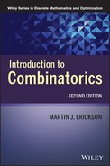
A chess Rook can move any number of squares horizontally or vertically on a chess board. How many different walks can a Rook travel in moving from the lower-left corner (al) to the upper-right corner (h8) on the board? Assume that the Rook moves right or up at every step. For example, Figure 2.1 shows the Rook walk al-cl-dl-d3-d5-f5-f7-h7-h8.
Figure 2.1 A Rook walk from al to h8.
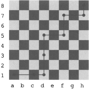
Note that if the Rook could only move one square at a time, this problem would be equivalent to the problem of counting paths along city streets (see Example 1.14). Here the number of such paths is simply ![]() = 3432. We expect that the number of Rook walks will be much larger.
= 3432. We expect that the number of Rook walks will be much larger.
Solution: We generalize the problem by considering Rook walks to any square on the board (with the Rook starting on al and moving toward the goal square at every step). We make a table displaying the number of walks. The bottom-left entry is the number of Rook walks from al to al, which is 1. Each other entry is the sum of all the entries below or to the left of the given entry. The reason is that the Rook’s last move must come from one of the squares represented by these entries. For example, the entry corresponding to the c4 square is 4 + 12 + 2 + 5 + 14 = 37. It’s possible to complete the table by hand in a few minutes. The number of Rook walks from a1 to h8 is 470,010. (The dots in the table indicate that we can generalize the problem to arbitrarily large chess boards.)
Let a(m, n) be the number of Rook walks from (0, 0) to (m, n), and set a(m, n) = 0 if m < 0 or n < 0. The generating function for the doubly infinite sequence {a(m, n)} is the rational function
(2.22) 
Can you explain why?
It follows that the sequence a(m, n) satisfies a recurrence relation (with initial values):

Can you explain why this recurrence relation holds by counting Rook walks?
Let an = a(n, n), for n ≥ 0. The sequence {an}, called the diagonal sequence, is
![]()
The eighth term, 470,010, is the number of Rook walks in the original problem.
Let f(x) be the generating function for the diagonal sequence, i.e.,
![]()
We will show that
(2.23) ![]()
In order to get the generating function for the diagonal sequence, we make the change of variables t = x/s. To include terms such as s3t5, we allow arbitrary integer exponents for s. For instance, we represent s3t5 as s−2x5. The diagonal generating function is the coefficient of s0. For more about this method, see [25].
We obtain the generating function
![]()
We now consider the function
![]()
Using the quadratic formula, we write this as
![]()
where
![]()
We put our function into partial fraction form,
![]()
or
![]()
For –1/9 < x < 1/9, we expand the function as a Laurent series in the annulus |α| < |s| < |β| in powers of α/s and s/β, obtaining
The coefficient of s0 in this series is
![]()
This establishes the generating function for the diagonal sequence.
We can use the generating function for the diagonal sequence to obtain a recurrence relation for it. By inspection,
![]()
We can read off a recurrence relation for {an} by looking at the coefficient of xn in the above relation:
(2.24) 
A counting argument for this relation is provided by E. Y. Jin and M. E. Nebel in “A combinatorial proof of the recurrence for rook paths,” in Electronic Journal of Combinatorics, 19, no. 1 (2012).
We can also use the generating function to determine the asymptotic growth rate of an. We have
(2.25) ![]()
See Exercises.
Can you find the generating function for the number of King walks from the lower-left corner to the upper-right corner of an arbitrary-size chess board? At each step, the King moves one square to the right, one square up, or both. Such walks are called Delannoy walks.
EXERCISES
![]()
![]()
![]()
![]()
![]()
2.3 Partition numbers
In Chapter 1, we defined the partition number p(n, k) to be the number of ways to write n as a sum of k positive integers. We can also think of p(n, k) as the number of onto functions f : X → Y, |X| = n, |Y| = k, where X and Y are unlabeled sets. Also, the partition number p(n) has been defined as p(n) = Σnk=1 p(n, k). In this section we develop generating functions for partition numbers.
EXAMPLE 2.8
Determine p(4, k), for k = 1, 2, 3, 4, and p(4).
Solution: We have
and
Suppose that X and Y are unlabeled and f : X → Y is an onto function (|X| = n, |Y| = k). Suppose that the inverse images of the elements of Y have cardinalities λ1, …, λk. Because the inverse images account for all the elements of X, it follows that
![]()
Furthermore, we may assume that the λi are ordered from largest to smallest:
![]()
A partition λ1 + · · · + λk = n may be pictured with a Ferrers diagram consisting of k rows of dots with λi dots in row i, where 1 ≤ i ≤ k. The Ferrers diagram for the partition 7 + 3 + 1 + 1 = 12 is shown in Figure 2.2.
Figure 2.2 The Ferrers diagram of a partition of 12.
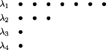
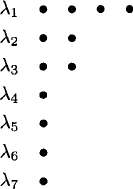
The transpose of a Ferrers diagram is created by writing each row of dots as a column. The resulting partition is called the conjugate of the original partition. For example, the partition 12 = 7 + 3 + 1 + 1 of Figure 2.2 is transposed to create the conjugate partition 12 = 4 + 2 + 2 + 1 + 1 + 1 + 1 of Figure 2.3.
Figure 2.3 A transpose Ferrers diagram.
The reader may enjoy matching each partition of 4 on the previous page with its conjugate. (One partition is self-conjugate.)
We now give the ordinary generating function for the partition numbers p(n). For convenience, we set p(0) = 1.
Proof. We need to show that the coefficients of xn on the two sides of the equation are equal. The coefficient of xn on the left side is patently p(n). On the right side, the product may be written as
To find the contribution to xn from this product, suppose the term xm(k)k is selected from the kth factor and these terms are multiplied to yield xm(1)+m(2)2+···. If this expression equals xn, then
Contributions to xn correspond to solutions of (2.26). These solutions may be envisioned as Ferrers diagrams for partitions of n. With t as the greatest integer for which m(t) is nonzero, we create the Ferrers diagram with m(t) rows of t dots, followed by m(t – 1) rows of t – 1 dots, etc. This correspondence between solutions of (2.26) and partitions of n completes the proof.
Determining the ordinary generating function for p(n, k) with k fixed is not difficult. We start by making an elementary observation from the transposes of Ferrers diagrams.
Theorem. The number of partitions of n into exactly k parts is equal to the number of partitions of n where the size of the greatest summand is k.
Now we can establish the generating function for p(n, k).
Theorem.
Proof We define p(n, ≤ k) to be the number of partitions of n into at most k parts. From the previous theorem, p(n, ≤ k) is also the number of partitions of n into parts of size at most k. Clearly, p(n, k) = p(n, ≤ k) – p(n, ≤ k – 1). We obtain
It follows that
Let p(n, O) be the number of partitions of n into summands each of which is an odd number. Let p(n, D) be the number of partitions of n into distinct summands. As a further illustration of the use of generating functions, we prove that p(n, O) = p(n, D).
Euler’s theorem (1748).
![]()
Proof. We have
The desired equality follows by comparing coefficients of the two generating functions.
EXERCISES
2.4 Labeled and unlabeled sets
Many enumeration problems can be solved by representing the objects to be counted as functions f : X → Y, where X and Y are chosen appropriately. The conditions imposed in the enumeration problem usually amount to putting restrictions on the functions (e.g., requiring them to be one-to-one) and/or making rules as to when two functions are considered equivalent (e.g., when they are equivalent up to a permutation of the elements of X). For example, the binomial coefficient ![]() is the number of 1–1 functions from an m-set X into an n-set Y, where the elements of X are considered to be indistinct.
is the number of 1–1 functions from an m-set X into an n-set Y, where the elements of X are considered to be indistinct.
Suppose that X and Y are two finite nonempty sets and Yx is the collection of functions f : X → Y. We wish to define some equivalence relations on Yx and, in each case, count the number of equivalence classes. When we say that two functions f and g(f, g ![]() YX) are equivalent, we will mean one of four things:
YX) are equivalent, we will mean one of four things:
(Note that the functions here are applied from right to left.)
In definitions (2) and (4) we say that h delabels X, and we speak of X as an unlabeled (or delabeled) set. Likewise, in definitions (3) and (4) we say that i delabels Y, and we speak of Y as an unlabeled or delabeled set.
EXAMPLE 2.9
Consider the functions f and g of Figure 2.4. Are they equivalent?
Figure 2.4 Two functions. Are they equivalent?
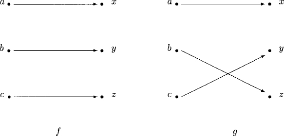
Solution: The functions fail to be equivalent under definition (1) because, after all, they are different functions. However, f = gh if h : X → X is the bijection given by h(a) = a, h(b) = c, and h(c) = b; therefore f and g satisfy definition (2). The bijection h rearranges the set {a, b, c}, eliminating the discrepancy between the two functions due to the labeling of the elements of the domain. If i is the bijection given by i(x) = x, i(y) = z, and i(z) = y, then f = ig; therefore f and g satisfy definition (3). It is now clear that the functions f and g of Figure 2.4 are equivalent according to definitions (2), (3), and (4).
EXAMPLE 2.10
Are the functions f and g of Figure 2.5 equivalent?
Figure 2.5 Equivalent functions when domain and codomain are unlabeled.
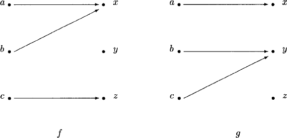
Solution: The functions f and g are equivalent only when both X and Y are unlabeled, i.e., according to definition (4). Define h: X → X by h(a) = c, h(b) = b, and h(c) = a, and define i: Y → Y by i(x) = z, i(y) = x, and i(z) = y. Then f = igh.
The domain and codomain of a function may be labeled or unlabeled sets, leading to four types of functions to be counted. Furthermore, functions may be classified according to whether they are one-to-one, onto, both, or not necessarily either. Altogether there are 16 cases, as shown in Table 2.2.
Table 2.2 The number of functions from X to Y, where |X| = m and |Y| = n.
We assume that f : X → Y is a function from a set X with m elements to a set Y with n elements. Let us consider the entries in the table, beginning with the X labeled, Y labeled box.
X labeled, Y labeled
We have already noted that the total number of such functions is nm.
As for the second entry, every one-to-one (1–1) function corresponds to an ordered selection of m objects from the set Y. There are n choices for the first object selected, n – 1 choices for the second, and so on, leading to the formula
![]()
If m > n, there are no one-to-one functions so we set P (n, m) = 0.
In the case of bijections, we either have two sets of the same cardinality or we don’t. If m ≠ n, then no bijection is possible. However, if m = n, then there are m! ways to match up the two sets. We define δ(m, n) to be 0 if m ≠ n and 1 if m = n. Thus, the number of bijections is m!δ(m, n). If either X or Y (or both) is unlabeled, then all bijections look the same, so the total number is δ(m, n).
X unlabeled, Y labeled
A one-to-one function f : X → Y is equivalent to a selection of m elements of Y without regard to order. The number of such selections is the value of the binomial coefficient
![]()
A function f : X → Y is equivalent to a distribution of m identical, elements (the elements of X) into n different boxes (the elements of Y). A box may receive any number of objects, including zero. Suppose we represent the m identical objects with m copies of the symbol *. The n boxes are represented by a set of n – 1 vertical lines|. The placement of the objects in the boxes is indicated by a linear ordering of the *’s and |’s. For example, * * * | * || * means that the first box (to the left of the first |) contains three objects, the second box contains one object, the third contains no objects, and the fourth contains one object. The total number of items in the linear ordering is m + n – 1, and n of these are |’s. Therefore, the total number of functions is
![]()
If f is onto, then each box must contain at least one object, and there are m – n objects to distribute freely. Hence, the number of onto functions is
![]()
Can you furnish a more direct combinatorial proof of this formula?
X labeled, Y unlabeled
If X is labeled and Y unlabeled, then the total number of functions from X to Y is the number of ways X may be partitioned into unlabeled parts (corresponding to the images under f). We prefer to define a formula only when m ≤ n, in which case the magnitude of n becomes unimportant (X can’t be divided into more than m parts). The Bell number B(m) is the number of such functions.
If m > n, then one-to-one functions do not exist. However, if m ≤ n, then all one-to-one functions look alike when X is unlabeled. This observation accounts for the 1–1 entries of the X unlabeled, Y labeled and X unlabeled, Y unlabeled boxes.
The number of onto functions when X is labeled and Y is unlabeled is ![]() , a Stirling number of the second kind. Clearly,
, a Stirling number of the second kind. Clearly,
![]()
as dividing by n! permutes the labels of the n sets into which X has been divided.
X unlabeled, Y unlabeled
The total number of functions when X and Y are unlabeled and m ≤ n is denoted p(m), and the values of p(m) are the partition numbers. The number of onto functions is the partition number p(m, n).
Four relations are obtained by comparing the total number of functions in each box of Table 2.2 to the number of onto functions. Thus
(2.29) 
The relation (2.27) follows from the fact that every function f : X → Y is onto some subset Y′ ![]() Y of cardinality j, where 1 < j ≤ m. The binomial coefficient
Y of cardinality j, where 1 < j ≤ m. The binomial coefficient ![]() “chooses” Y′ and T(m, j) counts the number of functions from X onto Y′. Relations (2.28) through (2.30) are proved similarly.
“chooses” Y′ and T(m, j) counts the number of functions from X onto Y′. Relations (2.28) through (2.30) are proved similarly.
EXERCISE
2.5 Counting with symmetry
We have classified functions f : X → Y (|X| = m, |Y| = n), where X and Y are labeled or unlabeled sets, and we enumerated these functions. Now we generalize the notion of labeled and unlabeled sets. For instance, recall that two functions f: X → Y and g : X → Y are equivalent in the X unlabeled, Y labeled sense if there exists a bijection h: X → X such that f = gh. The bijection h can be viewed as a permutation of X (in fact, any permutation in the symmetric group Sm.). What happens if we restrict the permutations to a specified subgroup G of Sm? If G is the identity group (e), for example, then we obtain the X labeled case; while if G = Sm, we obtain the X unlabeled case. Nontrivial subgroups G give rise to interesting intermediate cases. In these cases, Pólya’s theorem for the number of inequivalent functions allows us to count quite complicated configurations, including nonisomorphic graphs. (See Section 3.3 for definitions about graphs.) More generally, if one group G acts on X and another group H acts on Y, then the number of inequivalent functions is given by de Bruijn’s formula, which enumerates more intricate structures such as self-complementary graphs.
A group G is a nonempty set on which is defined a binary operation * satisfying the following three laws:
The element e is called the identity of G. The element x−1 is called the inverse of x. One can easily prove that the identity element of a group is unique and that the inverse x−1 of each element x is unique.
We sometimes indicate a group by an ordered pair, e.g., (G, *), to emphasize both the set and the operation. We usually suppress the group operation sign and write xy for x * y. We abbreviate xx by x2, x−1x−1 by x−2, etc. For any x ![]() G, we set x0 = e.
G, we set x0 = e.
EXAMPLE 2.11
The set Z is a group with respect to addition.
A finite group is a group with a finite number of elements, and the order of a finite group is the number of elements in it.
The cyclic group Zn, of order n, is the set {0,…,n – 1} under the clock addition operation * defined by x * y = x + y if x + y < n and x*y = x + y – n if x + y ≥ n.
A group G is abelian if xy = yx for all x, y ![]() G. Otherwise, G is nonabelian.
G. Otherwise, G is nonabelian.
EXAMPLE 2.12
The group Zn, is abelian.
The order of an element x ![]() G is the least positive integer n for which xn = e. If there is no such integer, then we say that x has infinite order.
G is the least positive integer n for which xn = e. If there is no such integer, then we say that x has infinite order.
EXAMPLE 2.13
In Z4, the elements 0, 1, 2, 3 have orders 1, 4, 2, 4, respectively.
The symmetric group Sn consists of the n! permutations of an n-set (e.g., Nn). The group operation * is composition of permutations. The elements of Sn are conveniently written in cycle notation. Thus,
![]()
is the element of S9 which maps 1 to 2 to 3 to 1, transposes 4 and 8, maps 3 to 6 to 7 to 3, and fixes 5 and 9. To multiply two permutations together, we just compute the result of the composition of the two bijections (reading left to right). For example,
![]()
Since (1 2)(1 3) ≠ (1 3)(1 2), the symmetric group Sn, is nonabelian for all n ≥ 3.
A homomorphism from one group (G1, *1) to another group (G2, *2) is a map f : G1 G2 which preserves multiplicative structure: f(x *1 y) = f(x) *2 f(y) for all x, y ![]() G1. If the homomorphism is a bijection we call it an isomorphism and say that the two groups G1 and G2 are isomorphic; we write G1
G1. If the homomorphism is a bijection we call it an isomorphism and say that the two groups G1 and G2 are isomorphic; we write G1 ![]() G2. A one-to-one homomorphism is called a monomorphism and an onto homomorphism is called an epimorphism. An isomorphism from a group G to itself is called an automorphism of G.
G2. A one-to-one homomorphism is called a monomorphism and an onto homomorphism is called an epimorphism. An isomorphism from a group G to itself is called an automorphism of G.
Suppose that G1 and G2 are two groups. The product of G1 and G2, denoted G1 × G2, is the set of ordered pairs {(g1, g2) : g1 ![]() G1, g2
G1, g2 ![]() G2} subject to the multiplication rule (g1, g2) * (g′1, g′2) = (g1g′1, g2g′2).
G2} subject to the multiplication rule (g1, g2) * (g′1, g′2) = (g1g′1, g2g′2).
EXAMPLE 2.14
The product Z2 × Z2 is a four-element group. It is not isomorphic to Z4, for Z2 × Z2 has three elements of order 2 and Z4 has only one.
We say that H is a subgroup of G if H is a subset of G and H is a group with respect to the group operation of G. We say that H is a normal subgroup of G if it is invariant under conjugation by elements of G, that is, xHx−1 = H for all x ![]() G.
G.
EXAMPLE 2.15
The two-element group {(1 2)(3), (1)(2)(3)} is a subgroup of the six-element group S3. It is not a normal subgroup. Why not?
The symmetric group Sn is especially important because every finite group is isomorphic to a subgroup of some Sn. This is Cayley’s theorem.
Cayley’s theorem (1854). If G is a finite group of order n, then G is isomorphic to a subgroup of Sn.
Proof. For each element g ![]() G, we define a function fg: G → G by the rule fg(a) = ag (right multiplication by g). Note that fg is a bijection because it has an inverse, namely, fg−1. We check: (fg
G, we define a function fg: G → G by the rule fg(a) = ag (right multiplication by g). Note that fg is a bijection because it has an inverse, namely, fg−1. We check: (fg ![]() fg−1)(a) = ag−1g = a and (fg−1
fg−1)(a) = ag−1g = a and (fg−1 ![]() fg)(a) = agg−1 = a. Since each fg is a permutation of the n-set G, we can define a map ϕ: G → Sn by ϕ(g) = fg. We claim that ϕ is a monomorphism. First we check that ϕ is an isomorphism: ϕ(gh)(a) = fgh(a) = a(gh) = (ag)h = fh(fg(a)) = (fgfh)(a) = (ϕ(g)ϕ(h))(a). Now we check that ϕ is one-to-one: If ϕ(g)(a) = ϕ(h)(a), then fg(a) = fh(a), which implies that ag = ah, and g = h.
fg)(a) = agg−1 = a. Since each fg is a permutation of the n-set G, we can define a map ϕ: G → Sn by ϕ(g) = fg. We claim that ϕ is a monomorphism. First we check that ϕ is an isomorphism: ϕ(gh)(a) = fgh(a) = a(gh) = (ag)h = fh(fg(a)) = (fgfh)(a) = (ϕ(g)ϕ(h))(a). Now we check that ϕ is one-to-one: If ϕ(g)(a) = ϕ(h)(a), then fg(a) = fh(a), which implies that ag = ah, and g = h.
The dihedral group Dn, of order 2n, consists of the set of symmetries of a regular n-gon. If we number the vertices of the n-gon 1,…,n, then we see that Dn is a subgroup of Sn. Specifically, the subgroup is generated by two permutations: the rotation r = (1 2 3 4 … n) and a flip f along an axis of symmetry of the n-gon. If n is odd we take the flip to be f = (n)(1 n – 1)(2 n – 2)(3 n – 3) … ![]() . If n is even we choose
. If n is even we choose ![]() . Each element of Dn can be written in the form ra fb, where a
. Each element of Dn can be written in the form ra fb, where a ![]() {1, n – 1} and b
{1, n – 1} and b ![]() {0, 1}. Two such elements are multiplied using the basic rules rn = e, f2 = e, and rf = fr−1. From these basic rules it is possible to compute all other products. We say that Dn has the presentation
{0, 1}. Two such elements are multiplied using the basic rules rn = e, f2 = e, and rf = fr−1. From these basic rules it is possible to compute all other products. We say that Dn has the presentation ![]() r, f : rn = 1, f2 = 1, rf = fr−1)
r, f : rn = 1, f2 = 1, rf = fr−1)![]() . For information about group presentations the reader should consult [17].
. For information about group presentations the reader should consult [17].
We have noted that every element of Sn can be expressed as a product of cycles. A cycle of length 2 is called a transposition and a cycle of length 1 is called a fixed point. Cycles of length greater than 2 can be written as products of transpositions. For example, (1 2 3) = (1 2)(1 3). A permutation may be written as a product of transpositions and fixed points in more than one way. However, the number of transpositions is always even or always odd. A permutation is accordingly called an even permutation or an odd permutation. It follows from the first homomorphism theorem for groups, to be discussed shortly, that Sn contains n!/2 even permutations and n!/2 odd permutations. (This fact follows more simply from the observation that f(σ) = (12)σ is a bijection between the set of even permutations of Sn and the set of odd permutations of Sn.) As the identity permutation is even and the even permutations are closed under multiplication and taking inverses, the even permutations are a group.
The alternating group An is the group of even permutations of the set { 1,…,n}. The group has order ![]() .
.
Let G be a group (with identity element e) and X a nonempty set. An action of G on X is a function θ: G × X → X which satisfies the following two conditions:
For convenience, we write θ(g, x) as gx, so that the two conditions become:
Remember, however, that g and h are group elements and x is a set element.
We note that each element g ![]() G yields a permutation of the set X (defined by sending x to gx). For if gx = gy, then x = y (hence the map is one-to-one) and gg−1 x = x (hence the map is onto).
G yields a permutation of the set X (defined by sending x to gx). For if gx = gy, then x = y (hence the map is one-to-one) and gg−1 x = x (hence the map is onto).
EXAMPLE 2.16
The symmetric group Sn, acts on Nn, by the natural action gx = g(x), where g(x) is the image of x under the function g: Nn → Nn.
EXAMPLE 2.17
The cyclic group Zn, acts on Nn by
Here g denotes the equivalence class representative of [g] that lies between 1 and n.
If x ![]() X, then the orbit of x (under the action θ) is orb(x) = {gx: g
X, then the orbit of x (under the action θ) is orb(x) = {gx: g ![]() G}. Orbits constitute equivalence classes of X; that is, X is partitioned into orbits. If there is only one orbit, then the action θ is transitive. Both examples above are transitive actions.
G}. Orbits constitute equivalence classes of X; that is, X is partitioned into orbits. If there is only one orbit, then the action θ is transitive. Both examples above are transitive actions.
To find the size of orb(x), note that gx = hx if and only if h−1 gx = x. Let Gx = {g ![]() G : gx = x}. We call Gx the stabilizer of x. We leave it to the reader to check that Gx is a normal subgroup G. Now gx = gy if and only if g
G : gx = x}. We call Gx the stabilizer of x. We leave it to the reader to check that Gx is a normal subgroup G. Now gx = gy if and only if g ![]() hGx, that is, if g and h are elements of the same coset of Gx. Therefore, the number of distinct values of gx is the number of cosets of Gx:
hGx, that is, if g and h are elements of the same coset of Gx. Therefore, the number of distinct values of gx is the number of cosets of Gx:
(2.31) ![]()
Let G be a finite group. For each g ![]() G, define fg: G → G by fg(x) = gxg−1. We say that G acts on itself by conjugation. The stabilizer of an element x
G, define fg: G → G by fg(x) = gxg−1. We say that G acts on itself by conjugation. The stabilizer of an element x ![]() G is called the centralizer of x and is denoted C(x). We call orb(x) the conjugacy class of x, and denote it by ccl(x). For the conjugacy action, we have
G is called the centralizer of x and is denoted C(x). We call orb(x) the conjugacy class of x, and denote it by ccl(x). For the conjugacy action, we have
(2.32) ![]()
Two permutations are in the same conjugacy class if and only if they have the same cycle structure. Therefore, the number of conjugacy classes equals the partition number p(n), where n = |G|.
Burnside’s lemma. Let G be a finite group acting on a finite nonempty set X. For each g ![]() G, let fg be the number of elements of X fixed by g. Then number of orbits n is given by
G, let fg be the number of elements of X fixed by g. Then number of orbits n is given by
Proof. The proof is a nice example of the technique of enumerating a set two different ways and comparing the results. The set is
![]()
On the one hand, by definition of fg, we have |S| = Σg![]() G fg. On the other hand, counting from the perspective of the elements of X and letting x′ denote orbit representatives, we have
G fg. On the other hand, counting from the perspective of the elements of X and letting x′ denote orbit representatives, we have
Equating the two expressions for |S|, we obtain ![]() , from which the desired relation follows instantly.
, from which the desired relation follows instantly.
EXAMPLE 2.18 Average number of fixed points of a permutation
How many fixed points has the average permutation of {1, 2, 3,…,n}? Recall that we solved this problem using probability in Example 1.27.
Solution: Applying Burnside’s lemma to the natural action of Sn, on Nn (which is transitive), we obtain
This is the average number of fixed points.
We now assume that f : X → Y is a function from a set X of m elements to a set Y of n elements. In the terminology of Pólya’s theory of counting, the elements of Y are labels, and f is a labeling of X. Suppose that a finite group G acts on X. We picture this situation with the following diagram:
![]()
This action of G on X induces an action of G on the set of labelings YX as follows: (gf)(x) = f(g−1 x) for all x ![]() X. We check the two axioms for an action:
X. We check the two axioms for an action:
The set YX of functions is partitioned into equivalence classes by this action. Functions in different equivalence classes are called G-inequivalent functions. By definition, the number of G-inequivalent functions is the number of orbits of the action of G on YX.
(2.33) 
Proof. Suppose that g, when regarded as a permutation of X, has cycle structure c = (c(1), c(2),…,c(m)). The functions fixed by g are precisely those which are constant on each cycle. As there are c(1) + · · · + c(m) cycles, each of which may be assigned one of n images, the number of functions fixed by g is fg = nc(1) + · · · + c(m). Our conclusion now follows directly from Burnside’s lemma.
EXAMPLE 2.19 Stacks of chips
How many stacks of 11 poker chips are possible with two colors of poker chips (red and white)?
Solution: Let X be the set of 11 positions in the stack and Y = {red, white}. The group S2 = {e, τ} acts on X, the identity e leaving the stack alone and τ turning the stack upside down. We need to know the cycle structures of e and τ. Certainly, e consists of 11 fixed points, so c(1) = 11 and c(i) = 0 for 2 ≤ i ≤ 11. And τ consists of one fixed point (the middle poker chip) and five transpositions, so c(1) = 1, c(2) = 5, and c(i) = 0 for 3 ≤ i ≤ 11. Therefore, the number of S2-inequivalent stacks is
![]()
EXAMPLE 2.20 Circular necklaces
How many 10-bead circular necklaces may be made using black or white beads?
Solution: Symmetries of the circular arrangement of beads are of six types: identity, rotations with one cycle, rotations with two cycles, rotations with five cycles, reflections through two opposite beads, and reflections through two opposite “sides?’ The number of necklaces is
![]()
While it is possible at this point to enumerate some rather complicated structures (nonisomorphic graphs, for instance), we prefer to do so only after developing some additional machinery—cycle indexes—in the next section.
EXERCISE
2.6 Cycle indexes
As in the previous section, we let c = (c(1),…,c(m)) be the cycle structure of g ![]() G when G acts on X (G finite, |X| = m). We assign to g the monomial
G when G acts on X (G finite, |X| = m). We assign to g the monomial
![]()
where the xi are variables in a commutative ring containing the rational numbers. The cycle index Z(G) is the average of these monomials:
(2.34) 
The cycle index Z(G) contains complete information about the cycle lengths of the various permutations g of the group action. George Pólya (1887–1985) chose the letter Z to stand for the German word Zycklenzeiger (“cycle indicator”). As Pólya said, “The cycle index knows many things.” For instance, letting each xi = n (a substitution denoted Z(G)[xi ← n]), we obtain the formula for the number of G-inequivalent functions in Yx |X| = m, |Y| = n):
(2.35) 
We next determine the cycle indexes of the most important group actions: En, Zn, Dn, Sn, An. The set acted upon is always X = {1,…n}.
The identity group En. The identity group consists of only the identity element e, which fixes every element of X. There are n 1-cycles, and the cycle index is
(2.36) ![]()
The cyclic group Zn. Given g ![]() G, x
G, x ![]() X, the length of the cycle containing x is the minimum positive k for which gk + x
X, the length of the cycle containing x is the minimum positive k for which gk + x ![]() x (mod n), or gk 0 (mod n). Because k is independent of x, all cycles of g have length k. If g contains j cycles, then jk = n, from which it follows that k is a divisor of n and j = n/k. To determine the number of elements g corresponding to each value of k, observe that k′n/k has order k whenever gcd(k′, k) = 1. There are ϕ(k) such values of k′, by definition of Euler’s ϕ-function. As Σk|n ϕ(k) = n, there are exactly ϕ(k) values of g for each k/n. Therefore
x (mod n), or gk 0 (mod n). Because k is independent of x, all cycles of g have length k. If g contains j cycles, then jk = n, from which it follows that k is a divisor of n and j = n/k. To determine the number of elements g corresponding to each value of k, observe that k′n/k has order k whenever gcd(k′, k) = 1. There are ϕ(k) such values of k′, by definition of Euler’s ϕ-function. As Σk|n ϕ(k) = n, there are exactly ϕ(k) values of g for each k/n. Therefore
The dihedral group Dn. As Dn contains Zn as a subgroup, the cycle index of Dn will contain all the terms in the formula (2.37). The other elements of Dn are “flips” (reflections). If n is odd, each flip fixes one element of X and contains (n – 1)/2 transpositions. If n is even, half of the flips contain n/2 transpositions and half contain two fixed points and (n – 2)/2 transpositions. Putting these facts together, we obtain the formulas
(2.38) 
The symmetric group Sn. A permutation g ![]() Sn can have any cycle structure c = (c(1),…,c(n)), where
Sn can have any cycle structure c = (c(1),…,c(n)), where
(2.39) ![]()
The number of solutions to this equation is a good counting puzzle in its own right. Solutions may be generated by ordering the elements of X and partitioning the elements from left to right into cycles of the appropriate lengths. Each of the n! orderings of X gives rise to repeated solutions due to interchanging cycles and writing cycles down in more than one way. Because there are c(k)! ways to list cycles of length k and each cycle may be written k ways, the number of solutions is
(2.40) ![]()
The cycle index of the symmetric group is
(2.41) ![]()
The alternating group An. The alternating group consists of the ![]() n! even permutations of Sn. When a permutation is written as a disjoint product of cycles, it is easy to tell whether it is even or odd. Because each odd cycle is equal to the product of an even number of transpositions, the number of odd cycles has no bearing on whether a permutation is even. However, each even cycle is equal to the product of an odd number of cycles. Hence, for a permutation to be even, it must be composed of an even number of disjoint cycles of even length. Therefore,
n! even permutations of Sn. When a permutation is written as a disjoint product of cycles, it is easy to tell whether it is even or odd. Because each odd cycle is equal to the product of an even number of transpositions, the number of odd cycles has no bearing on whether a permutation is even. However, each even cycle is equal to the product of an odd number of cycles. Hence, for a permutation to be even, it must be composed of an even number of disjoint cycles of even length. Therefore,
![]()
counts 1 for every even permutation and 0 for every odd permutation in Sn. This establishes the cycle index for the alternating group:
(2.42) ![]()
EXAMPLE 2.21 Circular necklaces (again)
How many 11-bead circular necklaces can be made with two types of beads?
Solution: The appropriate group is D11 acting on the set X = {1,…,11}. Hence
The only divisors of 11 are 1 and 11, for which ϕ(1) = 1 and ϕ(11) = 10. Thus
![]()
The number of necklaces that can be made with two types of beads is obtained by making the substitution
Recall that in Example 2.19 we determined that there are 1056 different stacks of 11 poker chips using two types of chips. The number of necklaces with 11 beads of two types is smaller because a necklace has more symmetries than a stack of chips.
EXERCISE
2.7 Pólya’s theorem
Pólya’s theorem. Let G act on X and therefore on the set of functions f : X → Y (G finite, |X| = m, |Y| = n). Suppose that F(y(1),…,y(n)) is the set of G-inequivalent functions for which |f−1(yi)| = y(i), where 1 ≤ i ≤ n. Then
where the right-hand sum is taken over all n-tuples (y(1),…,y(n)) with
Proof. We need to show that the coefficient of yy(1)1 · · · yy(n)n on the left side of the relation (2.43) is |F(y(1),…,y(n))|. By Burnside’s lemma,
(2.44) 
where fg is the number of functions in F(y(1),…,y(n)) fixed by g.
Suppose that g has cycle structure c = (c(1),…,c(n)). If the function
![]()
is fixed by g, then f is constant on each cycle of g; that is, each cycle of g lies entirely within one of the inverse images f−1(yi). Picture an m × 1 box (the elements of X) partitioned into n sections of sizes y(1),…,y(n) (the inverse images of f). Then fg is the number of possible packings of this box with c(i) blocks of sizes i, where 1 ≤ i ≤ m (the cycles of g). The polynomial on the left side of the relation (2.43) is
Let us consider how the ![]() terms are formed in the relation above. Suppose that each term
terms are formed in the relation above. Suppose that each term ![]() is expanded as a product of c(i) factors. Then each term in the product of these multiplicands is obtained by choosing a yii from each factor. The contribution to
is expanded as a product of c(i) factors. Then each term in the product of these multiplicands is obtained by choosing a yii from each factor. The contribution to ![]() is the number of ways the exponents (c(i) units of size i) may be arranged to equal y(i) for each 1 ≤ i ≤ n. These arrangements are clearly equivalent to the box packings described above. Therefore, the coefficient of
is the number of ways the exponents (c(i) units of size i) may be arranged to equal y(i) for each 1 ≤ i ≤ n. These arrangements are clearly equivalent to the box packings described above. Therefore, the coefficient of ![]() is
is
as we needed to show.
EXAMPLE 2.22 Circular necklaces (yet again)
Recall Example 2.20, which counted the number of circular necklaces with 10 beads, using black or white beads. How many such necklaces are made of seven white beads and three black beads?
Solution: The cycle index is
Making the substitution xi ← + yi1 + yi2 yields
![]()
We see that there are eight necklaces with seven white beads and three black beads. Can you sketch these eight necklaces?
EXAMPLE 2.23 Circular necklaces (one more time)
Making the substitution xi ← ai + 1 into Z(D11), we obtain the polynomial
![]()
(We use the term ai + 1 instead of yi1 + yi2 because it is simpler.) This polynomial tells us the number of 11-bead circular necklaces made of two types of beads, according to the number of beads of each type. For instance, there are 20 necklaces with seven white beads and four black beads.
EXERCISE
2.8 The number of graphs
In order to use Pólya’s theorem to count nonisomorphic graphs of order n, we need to determine the cycle index of the appropriate group action. A graph G = (V, E) may be identified with a function f : [V]2 → {0, 1}, where f({x, s}) = 1 or 0 according to whether or not {x, y} is a member of E. We say that two graphs G1 and G2 are isomorphic if there is a bijection between their vertex sets V1 to V2 that preserves adjacency. We normally regard two isomorphic graphs as the same graph. Two graphs are isomorphic if the corresponding functions are equal up to a permutation of V. As any permutation of V is allowed, the group acting on V is Sn, where n = |V|. This group induces an action on [V]2 by the rule {x, y} {gx, gy}. We call this action [Sn]2. Our goal is to calculate the cycle index Z([Sn]2).
Assume that g ![]() Sn has cycle structure c = (c(1),…,c(n)). We determine the cycle structure of g as a permutation of [V]2 by assuming that {x, y}
Sn has cycle structure c = (c(1),…,c(n)). We determine the cycle structure of g as a permutation of [V]2 by assuming that {x, y} ![]() [V]2 and examining four cases. We call the cycles in [V]2 pair-cycles.
[V]2 and examining four cases. We call the cycles in [V]2 pair-cycles.
Case 1. Suppose that x and y are in cycles of different lengths a and b. There are c(a) choices for which cycle contains x and c(b) choices for which cycle contains y. Given these choices, the ab ordered pairs in the Cartesian product of the two cycles are partitioned into pair-cycles of length lcm(a, b). The number of such cycles is ab/lcm(a, b) = gcd(a, b). The contribution to Z([Sn]2) is
Case 2. Suppose that x and y are in different cycles of the same length a. There are ![]() choices for the cycles. The pair-cycle has length a, and the number of pair-cycles is a. The contribution to Z([Sn]2) is
choices for the cycles. The pair-cycle has length a, and the number of pair-cycles is a. The contribution to Z([Sn]2) is
(2.46) 
Case 3. Suppose that x and y are in the same cycle of odd length a. There are c(a) choices for the cycle containing x and y and (a – 1)/2 choices for the gap between x and y. The pair-cycles all have length a. The contribution to Z([Sn]2) is
(2.47) ![]()
Case 4. Suppose that x and y are in the same cycle of even length a. This case is the same as Case 3 except for one important difference. There are still c(a) choices for the cycle containing x and y. But now, although the typical pair-cycle has length a, and there are (a – 2)/2 choices for the gap between x and y, there is also the possibility that x and y are a/2 units apart in the cycle, so that the pair-cycle has length a/2. The contribution to Z([Sn]2) is
(2.48) ![]()
Combining the formulas (2.45), (2.45), (2.45), and (2.45), we obtain a formula for the cycle index of [Sn]2:
The cycle indexes for 2 ≤ n ≤ 4 are easily calculated by hand:
(2.50) ![]()
(2.51) ![]()
(2.52) ![]()
Let’s examine the polynomial Z([S4]2). The 24 permutations of the set {1, 2, 3, 4} induce permutations of the six unordered pairs of elements. The identity permutation results in six fixed pairs. The six permutations of type 2 + 1 + 1 result in two fixed points and two 2-cycles in the set unordered pairs. The three permutations of type 2 + 2 result in two fixed points and two 2-cycles. The eight permutations of type 3 + 1 result in two 3-cycles. The six 4-cycles result in one 2-cycle and one 4-cycle.
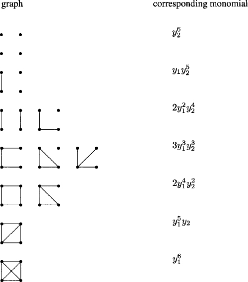
We apply Pólya’s theorem to the cycle index Z([S4]2) to enumerate nonisomorphic graphs of order 4 by number of edges:
The coefficient of yk1y6–k2 in this enumerating polynomial is the number of nonisomorphic graphs of order 4 with k edges and 6 – k non-edges. The symmetry in the polynomial comes from the fact that G and H are isomorphic if and only if their complements ![]() and
and ![]() are isomorphic.
are isomorphic.
We verify formula (2.53) by presenting in Figure 2.6 all nonisomorphic graphs of order 4 arranged by number of edges.
Figure 2.6 Graphs of order 4 and their enumerating monomials.
The total number of nonisomorphic graphs of order 4 is
The number of nonisomorphic graphs. The number of nonisomorphic graphs of order n is
![]()
Let g(n) be the number of nonisomorphic graphs on n vertices. Table 2.3 gives the value of g(n) for small n. We will show that
Table 2.3 The number of nonisomorphic graphs.
| order | number of graphs |
| 1 | 1 |
| 2 | 2 |
| 3 | 4 |
| 4 | 11 |
| 5 | 34 |
| 6 | 156 |
| 7 | 1044 |
| 8 | 12346 |
| 9 | 274668 |
| 10 | 12005168 |
Because ![]() is the number of labeled graphs, this means that almost all graphs have no nontrivial automorphisms. In fact, g(n) ~ c(n), where c(n) is the number of nonisomorphic connected graphs of order n. See [14].
is the number of labeled graphs, this means that almost all graphs have no nontrivial automorphisms. In fact, g(n) ~ c(n), where c(n) is the number of nonisomorphic connected graphs of order n. See [14].
Open problem. Find a formula for the number of nonisomorphic graphs of order n that contain a triangle.
Open problem. Find a formula for the number of nonisomorphic planar graphs of order n.
EXERCISE
Note that an is the number of involutions of an n-set and also the number of n × n symmetric permutation matrices. See Exercise 2.45.
2.9 Symmetries in domain and range
Suppose that X and Y are finite nonempty sets (|X| = m, |Y| = n) acted upon by finite groups G and H, respectively. We picture this situation with the following diagram:
![]()
We want to define what it means for two functions to be the same under these group actions. To this end, we define a new action HG on the set of functions YX = {f: X → Y} as follows: if g ![]() G, h
G, h ![]() H, and f
H, and f ![]() YX, then (hg f)(x) = hf (g−1 x). (The reader should check that the two axioms for a group action are satisfied.) We say that two functions are equivalent if they are in the same orbit of the action and inequivalent otherwise. This definition is a generalization of the labeled/unlabeled set paradigm. If G is the symmetric group Sm, then X is unlabeled, and if G is the identity group Em, then X is labeled. Likewise, if H is Sn, then Y is unlabeled, and if H is En, then Y is labeled. For any groups G and H, Burnside’s lemma gives the number of inequivalent functions:
YX, then (hg f)(x) = hf (g−1 x). (The reader should check that the two axioms for a group action are satisfied.) We say that two functions are equivalent if they are in the same orbit of the action and inequivalent otherwise. This definition is a generalization of the labeled/unlabeled set paradigm. If G is the symmetric group Sm, then X is unlabeled, and if G is the identity group Em, then X is labeled. Likewise, if H is Sn, then Y is unlabeled, and if H is En, then Y is labeled. For any groups G and H, Burnside’s lemma gives the number of inequivalent functions:
where Ω(g, h) is the number of functions fixed by hg.
If f is fixed by hg, then f(g−1 x) = hf(x) for all x ![]() X. Thus f(x) = y implies that f(g−1 x) = hf(x) = hy, which in turn implies that f(g−2 x) = h2y. In general, f(g−i x) = hi y. It follows that if x is in a cycle of length i in g and y is in a cycle of length j in h, then j divides i. Furthermore, we have shown that the correspondence between the two cycles is completely determined by the relation f(x) = y. There are j choices for the image of x. Suppose that g has cycle structure (c(1),…,c(m)) and h has cycle structure (d(1),…,d(n)). Then, given i and a particular cycle of length i in g, the number of fixed functions is
X. Thus f(x) = y implies that f(g−1 x) = hf(x) = hy, which in turn implies that f(g−2 x) = h2y. In general, f(g−i x) = hi y. It follows that if x is in a cycle of length i in g and y is in a cycle of length j in h, then j divides i. Furthermore, we have shown that the correspondence between the two cycles is completely determined by the relation f(x) = y. There are j choices for the image of x. Suppose that g has cycle structure (c(1),…,c(m)) and h has cycle structure (d(1),…,d(n)). Then, given i and a particular cycle of length i in g, the number of fixed functions is
(2.55) ![]()
and the total number of fixed functions is
Formulas (2.54) through (2.56) combine to yield the following formula of N. G. de Bruijn (1918–2012).
De Bruijn’s formula. If finite groups G and H act on finite nonempty sets X and Y, respectively, then the number of inequivalent functions is given by
(2.57) 
We apply de Bruijn’s formula to the problem of counting self-symmetric graphs of order n, that is, graphs G for which G is isomorphic to its complement ![]() . In the previous section we determined the cycle index Z([Sn]2) and the number of nonisomorphic graphs of order n, i.e., g(n) = Z([Sn])[xi ← 2]. If [Sn]2 acts on the set X = {1,…,n} and S2 acts on Y = 11, then functions correspond to nonisomorphic graphs where G and its complement
. In the previous section we determined the cycle index Z([Sn]2) and the number of nonisomorphic graphs of order n, i.e., g(n) = Z([Sn])[xi ← 2]. If [Sn]2 acts on the set X = {1,…,n} and S2 acts on Y = 11, then functions correspond to nonisomorphic graphs where G and its complement ![]() are regarded as the same. Hence, the number of such functions is
are regarded as the same. Hence, the number of such functions is
(2.58) 
Let g* (n) be the number of self-complementary graphs of order n. As 2N(n) counts nonisomorphic graphs with each self-complementary graph counted twice, we obtain the formula
(2.59) ![]()
For example, g*(4) = 2N(4) – g(4) = 2 · 6 – 11 = 1, and the unique self-complementary graph of order 4 is the path P4.
EXERCISE
2.10 Asymmetric graphs
Our formula for the number of nonisomorphic graphs of order n is
(2.60) ![]()
where c = (c1,…,cn) is the cycle type of a permutation of {1,…,n}, the number of permutations of such a cycle type is
(2.61) ![]()
and
(2.62) 
We will prove that
(2.63) ![]()
This result means that the typical unlabeled graph has no nontrivial symmetries and hence is an asymmetric graph.
The lower bound is trivial:
![]()
Now we prove the upper bound. Assume that the permutation has n – j fixed points, where 0 ≤ j ≤ n. The case j = 0 gives the term ![]() !. We will show that the other terms are bounded above by expressions which, upon division by
!. We will show that the other terms are bounded above by expressions which, upon division by ![]() !, tend to 0 as n → ∞.
!, tend to 0 as n → ∞.
We have
The number of permutations with n – j fixed points is bounded above by
The case j = 2 yields the exponent
Upon dividing by ![]() , the contribution is bounded by 2−n+2+2 log2 n, which tends to 0 as n → ∞.
, the contribution is bounded by 2−n+2+2 log2 n, which tends to 0 as n → ∞.
Now let’s look at the case j ≥ 3, so that 1 – j/2 < O. We obtain
and
![]()
Upon dividing by ![]() !, the contribution is bounded by 2
!, the contribution is bounded by 2![]() n(1–j/2)+j log2 n, which tends to 0 as n → ∞.
n(1–j/2)+j log2 n, which tends to 0 as n → ∞.
Erd![]() s and Rényi theorem (1963). Almost all unlabeled graphs are asymmetric:
s and Rényi theorem (1963). Almost all unlabeled graphs are asymmetric:
EXERCISE
Notes
The notation for falling factorial and rising factorial varies considerably. The falling factorial function is often written (x)n.
James Sylvester (1814–1897) introduced the notion of Ferrers diagrams in 1853. Apparently they were discovered by Norman Ferrers (1829–1903).
G. H. Hardy and Srinivasa Ramanujan (1887–1920) were the first mathematicians to find an explicit formula for p(n). The most elementary asymptotic estimate is loge p(n) ~ π(2n/3)1/2. See [12] for details.
In 1937 George Pólya (1887–1985) published the formula for enumerating graphs in connection with a problem concerning the number of chemical isomers. The language of his counting theory was quite descriptive. A function from X to Y is called a configuration. The elements of X are places and the elements of Y are figures. The store inventory is ![]() and the pattern inventory is
and the pattern inventory is ![]() . Thus the basic problem is to find the number of G-inequivalent patterns. An alternative approach to the Pólya theory of counting was undertaken independently by John H. Redfield (1879–1944) in 1927.
. Thus the basic problem is to find the number of G-inequivalent patterns. An alternative approach to the Pólya theory of counting was undertaken independently by John H. Redfield (1879–1944) in 1927.