
CHAPTER 5
ERROR-CORRECTING CODES
Sixteen unit hyperspheres can be arranged in R7 so that each hypersphere is tangent to exactly seven of the other hyperspheres.
This configuration of spheres is called a perfect packing. How do we obtain such a packing? What makes it perfect? What are its combinatorial properties? In this chapter and the next, we investigate such combinatorial designs, paying close attention to the interrelationships among the constructions and often finding equivalences between seemingly different structures. As a capstone, we construct the (23, 212, 7) Golay code G23, the S(5, 8, 24) Steiner system, and Leech’s 24-dimensional lattice L. We begin our tour of combinatorial constructions with practical examples called codes.
5.1 Binary codes
Let F = {0, 1}, the field of two elements. Then Fn, the collection of strings of length n over F, is a vector space of dimension n over F. We can picture Fn as the set of vertices of the n-dimensional unit hypercube. For example, Figure 5.1 depicts F3 as the set of vertices of the cube. These vertices are coordinatized with the eight vector representatives 000, 001, 010, 011, 100, 101, 110, and 111. Note that two vertices are edge adjacent if and only if their vector representatives differ in exactly one coordinate.
Figure 5.1 F3 as the set of vertices of a cube.

Given any two binary strings v, w ![]() Fn, we define the Hamming distance d(v, w) between v and w to be the number of coordinates where v and w differ. This is also the shortest edge path in the hypercube between x and y. For example, we can see in Figure 5.1 that d(011, 101) = 2.
Fn, we define the Hamming distance d(v, w) between v and w to be the number of coordinates where v and w differ. This is also the shortest edge path in the hypercube between x and y. For example, we can see in Figure 5.1 that d(011, 101) = 2.
The function d is a metric, which we call the Hamming metric or Hamming distance, and Fn is a metric space.
Theorem. The function d is a metric on Fn; that is, for all v, w, x ![]() Fn, the following properties hold:
Fn, the following properties hold:
Proof. Properties (1) and (2) are immediate from the definition of d. We prove the triangle inequality by verifying that it is preserved componentwise. Let vi, wi, xi be the ith components of the vectors v, w, x, respectively. If vi = wi = xi, then the contribution to both sides of the inequality is 0. If not, then the contribution to the left side is at least 1 while the contribution to the right side is at most 1. Hence, the inequality is preserved componentwise. (It is also easy to “see” that d is a metric by realizing that d(x, y) is the shortest path length between x and y along the edges of a cube embedded in Rn.)
The weight w(v) of a vector v is the number of 1′s in the vector representation of v. A simple componentwise proof demonstrates that d(x, y) = w(x – y) for any x, y ![]() Fn.
Fn.
The Hamming sphere with radius r and center c is the set of all v ![]() Fn such that d(v, c) ≤ r. The volume of the sphere is the number of elements in it:
Fn such that d(v, c) ≤ r. The volume of the sphere is the number of elements in it: ![]() . Note that
. Note that ![]() counts selections of the k coordinates in which c and v disagree.
counts selections of the k coordinates in which c and v disagree.
It is difficult to picture spheres when n is large (and they don’t look very spherical). We will mainly be interested in how densely they can be packed, because, as we shall see, dense packings signify good codes.
A code A is a subset of Fn with |A| ≥ 2. The elements of A are called codewords. In real-life applications, information can be sent reliably over a noisy channel by encoding redundancy in the message. A codeword v ![]() A is transmitted and a possibly distorted vector v′ is received. As it might happen that v′ equals a codeword in A different from v, it is not always possible to tell whether any errors have been committed in the transmission. However, if the Hamming distances between pairs of codewords are fairly large (which is achievable with redundancy), it is unlikely that v′ will equal another codeword. If the Hamming distances are large enough, it may be possible to detect errors when they occur and correct them.
A is transmitted and a possibly distorted vector v′ is received. As it might happen that v′ equals a codeword in A different from v, it is not always possible to tell whether any errors have been committed in the transmission. However, if the Hamming distances between pairs of codewords are fairly large (which is achievable with redundancy), it is unlikely that v′ will equal another codeword. If the Hamming distances are large enough, it may be possible to detect errors when they occur and correct them.
The distance d(A) of a code A is the minimum Hamming distance between distinct codewords in A. For example, the code A = {011, 101, 110} ![]() F3 has distance d(A) = 2, because any two of the vectors in A differ by two bits. It is always true that 1 ≤ d(A) ≤ n.
F3 has distance d(A) = 2, because any two of the vectors in A differ by two bits. It is always true that 1 ≤ d(A) ≤ n.
A code with distance d = e + 1 detects e errors. A code with distance d = 2e + 1 corrects e errors. To justify these definitions, suppose that a codeword v is sent and a string v′ is received, with 1 ≤ d(v, v′) ≤ e. If d = e + 1, then v′ cannot equal some codeword x or else d(v, v′) ≥ e + 1, a contradiction. Therefore, we can detect that at least one error has occurred. If d = 2e + 1, then v′ cannot have resulted from the transmission of an erroneous codeword x (and at most e errors), or else ![]() , a contradiction. Therefore, we can identify the particular vector v that was sent and correct the errors.
, a contradiction. Therefore, we can identify the particular vector v that was sent and correct the errors.
 EXAMPLE 5.1 Triplicate code
The code {000, 111} ![]() F3 is called a triplicate code. Under the map 0
F3 is called a triplicate code. Under the map 0 ![]() 000 and 1
000 and 1 ![]() 111, each bit is tripled. If an error occurs (a bit is switched from 0 to 1 or 1 to 0), then we can still tell which message was intended. Thus, the code has distance 3 and is capable of correcting one error. If a codeword is transmitted and we receive 001, then, under the assumption that at most one error has been committed, the intended word must be 000. Let q be the probability that a bit is mistakenly altered from 0 to 1 or from 1 to 0, and suppose that bits are altered independently of each another. The decoding scheme fails if two or three errors occur, and this happens with probability 3q2(1 – q) + q3, which is asymptotic to 3q2 for q small. This probability of failure is much smaller than the probability q of failure when no code is used. However, the increase in reliability is paid for by a decrease in transmission rate. The rate r(A) of a code A, defined as r(A) = log2 |A|/n, measures the amount of information per code bit conveyed over the communication channel. Always, 1/n ≤ r(A) ≤ 1. In the above example, r(A) =- (log2 2)/3 = 1/3, which means that when information is sent in triplicate the rate decreases by a factor of 3 (which is reasonable).
111, each bit is tripled. If an error occurs (a bit is switched from 0 to 1 or 1 to 0), then we can still tell which message was intended. Thus, the code has distance 3 and is capable of correcting one error. If a codeword is transmitted and we receive 001, then, under the assumption that at most one error has been committed, the intended word must be 000. Let q be the probability that a bit is mistakenly altered from 0 to 1 or from 1 to 0, and suppose that bits are altered independently of each another. The decoding scheme fails if two or three errors occur, and this happens with probability 3q2(1 – q) + q3, which is asymptotic to 3q2 for q small. This probability of failure is much smaller than the probability q of failure when no code is used. However, the increase in reliability is paid for by a decrease in transmission rate. The rate r(A) of a code A, defined as r(A) = log2 |A|/n, measures the amount of information per code bit conveyed over the communication channel. Always, 1/n ≤ r(A) ≤ 1. In the above example, r(A) =- (log2 2)/3 = 1/3, which means that when information is sent in triplicate the rate decreases by a factor of 3 (which is reasonable).
We refer to a code A ![]() Fn with distance d(A) = d as an (n, |A|, d) code. The number n is sometimes called the dimension of the code, and |A| is called the size of the code. Let there be no confusion between the distance d (an integer) and the Hamming metric d (a function).
Fn with distance d(A) = d as an (n, |A|, d) code. The number n is sometimes called the dimension of the code, and |A| is called the size of the code. Let there be no confusion between the distance d (an integer) and the Hamming metric d (a function).
For n fixed, there is an inverse relationship between |A| and d (and therefore between the rate and the error-correcting capability of the code). The fundamental problem of coding theory is to find codes with high rate and large distance. The next theorem gives sharp focus to this problem.
Hamming upper bound. If A corrects e errors, then
(5.1) ![]()
Proof. Because d ≥ 2e + 1, the spheres of radius e centered at the codewords do not intersect. Therefore, the total volume of the spheres is at most the cardinality of Fn; that is,
from which the upper bound follows instantly.
The Hamming upper bound for |A| is also called the sphere packing bound.
EXERCISES
5.2 Perfect codes
If the Hamming upper bound is achieved for a code A, we say that A is perfect. Perfect codes correspond to sphere packings of Fn with no wasted space (vectors not in a sphere). If A is perfect, then ![]() must divide 2n and hence be a power of 2. We will soon see that this rarely happens.
must divide 2n and hence be a power of 2. We will soon see that this rarely happens.
If |A| = 2, then the maximum value of d(A) is n and this value is achieved, for instance, when A consists of the all-0 vector and the all-1 vector. If |A| > 2, then some two vectors must agree on any given component, so d(A) < n. Therefore, n > d ≥ 2e + 1, which implies that
(5.2) ![]()
If e = 1, then ![]() = 1 + n, which is a power of 2 when n = 2r – 1 for some r ≥ 2. In this case, |A| = 2n/2r = 2n–r = 2m, where m = n – r = 2r – 1 – r. Hence, the parameters of such a code are (n, |A|, d) (2r – 1, 2m, 3).
= 1 + n, which is a power of 2 when n = 2r – 1 for some r ≥ 2. In this case, |A| = 2n/2r = 2n–r = 2m, where m = n – r = 2r – 1 – r. Hence, the parameters of such a code are (n, |A|, d) (2r – 1, 2m, 3).
The next theorem says that there are only two feasible sets of parameters for perfect codes when 1 < e < (n – 1)/2. This was proved by Aimo Tietäväinen and J. H. van Lint (1932–2004). Unfortunately, no simple proof of this fact is known. Their proof uses the theory of equations and is quite complicated. See [22].
Theorem. The only values of n and e for which 1 < e < ![]() and
and ![]() is a power of 2 are (n, e) = (23, 3) and (90, 2).
is a power of 2 are (n, e) = (23, 3) and (90, 2).
These values correspond to two special sums of binomial coefficients:
If there are codes with these values of n and e, they would have parameters (n, |A|, d) = (23, 212, 7) and (90, 278, 5). We outline a proof in the exercises that there is no code with parameters (90, 278, 5). A code with parameters (23, 212, 7), called the Golay code G23, is constructed in Section 6.7.
We have taken the base field of our codes to be GF(2), but if we allow other base fields, it turns out that there is only one more perfect code, the ternary code G11 with parameters (11, 36, 5), discovered by Marcel Golay. If we consider any alphabet as the base set (not necessarily a field), then a perfect code is one of the two Golay codes G23 and G11 or else has the parameters of a Hamming code.
In the next section, we will describe the Hamming codes, a family of perfect 1-error-correcting codes.
EXERCISES
![]()
5.3 Hamming codes
As in the previous section, we define n = 2r – 1 and m = 2r – 1 – r, where r ≥ 2. If r = 2, then n = 3 and m = 1, and the vertices 000 and 111 of the cube C3 of Figure 5.1 constitute such a code. We now describe a code A ![]() Fn with |A| = 2m that corrects one error, exhibiting a construction in the case r = 3, n = 7, m = 4. The constructions for r > 3 are carried out similarly.
Fn with |A| = 2m that corrects one error, exhibiting a construction in the case r = 3, n = 7, m = 4. The constructions for r > 3 are carried out similarly.
Let
(5.3) 
be the r × n = 3 × 7 matrix whose columns are the numbers 1,…,n written in binary. The matrix H represents a linear transformation from F7 to F3:
![]()
We define the code A to be the kernel of H; that is,
(5.4) ![]()
(The 0 here is the 3 × 1 zero vector.) We call H a parity check matrix for A. Any code A for which x ![]() A and y
A and y ![]() A imply x + y
A imply x + y ![]() A is called a linear code. Clearly, a code described as the kernel of a parity check matrix is a linear code.
A is called a linear code. Clearly, a code described as the kernel of a parity check matrix is a linear code.
By inspection, we find two of the vectors belonging to A:
As the Hamming distance between these two vectors is 3, we see that d(A) ≤ 3. We need to prove that d(A) ≥ 3 and |A| = 2m = 16.
Assume that v = [x y a z b c d]t ![]() A. (The reason for the nonalphabetical listing of the components of v will become clear in a moment.) Because v is in the kernel of H, we have Hv = 0. Thus
A. (The reason for the nonalphabetical listing of the components of v will become clear in a moment.) Because v is in the kernel of H, we have Hv = 0. Thus
(5.5) 
which yields three equations
Because we are working in, F, we have –x = x for all x, and the equations becomes
(5.6) 
The variables a, b, c, d may independently take either value, 0 or 1, in F. For this reason they are called free variables. There are 24 choices for the values of the four free variables. The variables x, y, z are determined by these choices and are therefore called determined variables. The values of the free variables are called information bits, while the values of determined variables are called check bits.
We have shown that |A| = 16. It remains to prove d(A) ≥ 3, which we do by showing that A corrects one error. Suppose that a codeword c ![]() A is sent and one error occurs. Assuming that the error occurs in the ith component, we represent the error by a vector consisting of a single 1 in the ith position and 0′s in all other positions:
A is sent and one error occurs. Assuming that the error occurs in the ith component, we represent the error by a vector consisting of a single 1 in the ith position and 0′s in all other positions:
The received vector is c + e (which differs from c in just the ith component), and it is the decoder’s job to determine the position in which the error has occurred. This is done by exploiting properties of the matrix H. We multiply H by c + e:
Since e has only one nonzero row, the product He consists of the column of H corresponding to this row position. In other words, He equals the ith column of H. Because of the way H is constructed, this is the number i in binary. Thus, when we compute H(c + e) the position of the error is revealed (in binary). We have demonstrated that A corrects one error, so d(A) ≥ 2 · 1 + 1 = 3.
We have already remarked that A is a perfect code. As a sphere packing, A may be pictured as the centers of the spheres (in Euclidean space) referred to in the introduction to this chapter. As we have already noted, every element of F3 lies in exactly one sphere. This Hamming code (of dimension 7) has rate r(A) = (log2 16)/7 = 4/7. In general, the Hamming code of dimension n has rate
(5.7) ![]()
which tends to 1 as r tends to infinity. Thus, the Hamming codes are a family of 1-error-correcting codes with arbitrarily good rate.
The equations of the previous section allow us to determine the 16 codewords of the (7, 16, 3) Hamming code. They are listed below:
Since d(x, y) = w(x – y) for any x, y ![]() Fn, the distance of a linear code equals the minimum weight of a nonzero codeword. Table 5.1 tallies the words of the (7, 16, 3) Hamming code according to weight.
Fn, the distance of a linear code equals the minimum weight of a nonzero codeword. Table 5.1 tallies the words of the (7, 16, 3) Hamming code according to weight.
Table 5.1 Weight distribution of the Hamming code.
The symmetry of the weight distribution is due to the fact that A is a linear code containing the all-1 codeword. Thus, if v ![]() A, then also vc
A, then also vc ![]() A (where vc is the binary complement of v) and w(vc) = 7 – w(v).
A (where vc is the binary complement of v) and w(vc) = 7 – w(v).
The seven Hamming codewords of weight 3 give rise to a finite geometry called the Fano Configuration (FC). The Fano Configuration has seven points, 1, 2, 3, 4, 5, 6, 7, corresponding to the seven components of the code vectors of A. Each codeword of weight 3 contains, by definition, three 1′s. The three points corresponding to the 1′s are joined by a line, called an edge of FC. The edges are 246, 167, 145, 257, 123, 347, and 356.
EXERCISES
5.4 The Fano Configuration
The simplest combinatorial construction is known as the Fano Configuration, named after the geometer Gino Fano (1871–1952)1. The Fano Configuration is the prototypical example of many types of structures, such as projective planes, block designs, and difference sets. Let’s look at the configuration and observe some of its properties.
The Fano Configuration (FC) is shown in Figure 5.2.
Figure 5.2 The Fano Configuration (FC).

The points of FC are labeled 1, 2, 3, 4, 5, 6, and 7. The lines are just unordered triples of points (e.g., {1, 2, 3}); they have no Euclidean meaning Hence, the points may be located anywhere in space, and the lines may be drawn straight or curved and may cross arbitrarily.
We observe that FC has the following properties:
The above properties occur in pairs called duals. If the words “point” and “line” are interchanged, each property is transformed into its dual property.
FC has many fascinating properties. For instance, with its edges properly oriented, FC represents the multiplication table for the Cayley algebra. Here is a simple application.
EXAMPLE 5.2
Seven students are asked to evaluate a set of seven textbooks, making comparisons between pairs of textbooks. While it is possible for every student to read every book and write comparisons between each pair, this would be time consuming. Instead, each student receives three books to read, according to the FC diagram. Number the students 1, 2, 3, 4, 5, 6, 7. The books correspond to the lines and therefore can be numbered {1, 2, 3}, {2, 4, 6}, etc. Then, for example, student 2 receives books {1, 2, 3}, {2, 4, 6}, and {2, 5, 7}. Each student writes a comparison between the three pairs of books that he or she reads. Thus, each student must write only three comparisons, instead of 21.
We next determine the automorphism group of FC, denoted Aut FC. This automorphism group is the group of permutations of the vertices of FC that preserve collinearity. For example, if we rotate FC clockwise by one-third of a circle, collinearity is preserved. This permutation is written in cycle notation as (142)(356)(7).
We begin by calculating the order of Aut FC. It is evident from Figure 5.2 that all seven vertices are equivalent in terms of collinearity. Therefore, vertex 1 may be sent by an automorphism to any of the seven vertices. Suppose that 1 is mapped to 1′. Vertex 2 may be mapped to any of the remaining six vertices. Suppose that 2 is mapped to 2′. In order to preserve collinearity, vertex 3 must be mapped to the unique point collinear with 1′ and 2′. Call this point 3′. Vertex 4 is not on line 123, so its image 4′ can be any of the remaining four vertices. Finally, the images of the other points are all determined by collinearity: 5 is collinear with 1 and 4; 6 is collinear with 2 and 4; and 7 is collinear with 3 and 4. Hence, there are 7·6·4 = 168 automorphisms.
Now we know that Aut FC is a group of order 168, but what group? Is it abelian? Cyclic? Simple? We will show that Aut FC is isomorphic to the group of invertible 3 × 3 matrices over F.
Here is some background about groups of matrices. The general linear group GL(n, q) is the set of invertible n × n matrices with coefficients in the Galois field GF(q) of order q = pk, where p is a prime, under matrix multiplication. The order of GL(n, q) is readily determined. There are qn – 1 choices for the first row of an invertible n × n matrix (the all-0 row is excluded). Having chosen the first row, the second row may be any of the qn possible n-tuples except the q scalar multiples of the first row. Hence, there are qn – q choices for the second row. Similarly, the third row may be any of the qn n-tuples except linear combinations of the first two rows. There are qn – q2 choices. Continuing in this manner, we arrive at the total number of invertible matrices:
(5.8) ![]()
For example, GL(2, 2) has six elements and is in fact isomorphic to S3. The group Aut FC is isomorphic to GL(3, 2).
The special linear group SL(n, q) is a subgroup of GL(n, q) consisting of those n × n invertible matrices with entries from GF(q) and determinant 1. We claim that SL(n, q) is a normal subgroup of GL(n, q). For if M ![]() SL(n, q) and N
SL(n, q) and N ![]() GL(n, q), then
GL(n, q), then
![]()
Now consider the homomorphism
![]()
The kernel of f is SL(n, q) and the homomorphism is clearly onto. Therefore, by the first homomorphism theorem for groups,
(5.9) ![]()
and hence,
(5.10) ![]()
Projective versions of the groups GL(n, q) and SL(n, q) are obtained as the quotient groups of these groups by their centers. The projective general linear group PGL(n, q) is GL(n, q)/Z(GL(n, q)) and the projective special linear group PSL(n, q) is SL(n, q)/Z(SL(n, q)). In the exercises, the reader is asked to prove the following formulas:
and
where d = gcd(n, q – 1).
For all n ≥ 1, we have
![]()
When n = 3 we obtain
![]()
We will now show that Aut FC is isomorphic to GL(3, 2).
We label the vertices of FC with the seven nonzero vectors in F3, as in Figure 5.3. This labeling is derived from the labeling of Figure 5.2 by assigning to each vertex i the vector that represents the number i in binary. The vectors have been chosen so that v1, v2, v3 are collinear if and only if v1 + v2 + v3 = 0 (in F3). The matrix group GL(3, 2) acts on the vectors of FC in the obvious way: v ![]() vM. It is easy to check that this action preserves collinearity: v1 + v2 + v3 = 0 if and only if (v1 + v2 + v3)M = 0 · M, which is true if and only if v1M + v2M + v3M = 0. Therefore, Aut FC is isomorphic to the group of 3 × 3 invertible matrices over F.
vM. It is easy to check that this action preserves collinearity: v1 + v2 + v3 = 0 if and only if (v1 + v2 + v3)M = 0 · M, which is true if and only if v1M + v2M + v3M = 0. Therefore, Aut FC is isomorphic to the group of 3 × 3 invertible matrices over F.
Figure 5.3 A vector representation of FC.

It is well known (see [23]) that PSL(n, q) is a simple group (a group with no nontrivial normal subgroups) for all n ≥ 2 except n = 2 and q = 2 or q = 3. Because there is only one nonabelian group of order 6, it follows that PSL(2, 2) ![]() S3. It is also easy to show that PSL(2, 3)
S3. It is also easy to show that PSL(2, 3) ![]() A4. The simple groups are crucial to the study of algebra. Some of them are difficult to describe, although we have shown that PSL(3, 2) (
A4. The simple groups are crucial to the study of algebra. Some of them are difficult to describe, although we have shown that PSL(3, 2) (![]() GL(3, 2)) has a nice geometric model.
GL(3, 2)) has a nice geometric model.
Let us find generators for Aut FC. By direct calculation, we see that the rows of M are the images of the binary representations of 1, 2, and 4. Let
We observe from Figure 5.3 that T yields a reflection of FC around the 374 axis while S yields the 7-cycle (1 5 6 7 2 4 3). We will show that all 168 matrices in the automorphism group of FC are generated by combinations of S and T.
The “visible automorphisms” of FC are the symmetries of its equilateral triangular shape given by the elements of the symmetric group S3. These symmetries are combinations of S and T, for T is a reflection of the triangle (i.e., a transposition of two of its vertices) and (S2TS2)2T is a rotation of the triangle by one-third of a circle; all symmetries of the triangle are combinations of a reflection and a rotation. Furthermore, STS2T is a transvection (the identity matrix with an extra 1 in an off-diagonal position). From the transvection, we can produce all transvections via conjugation by permutations. Using elementary row operations, all invertible matrices can be formed from permutation matrices and transvections. Therefore, all invertible matrices are combinations of S and T.
A presentation of the group is
![]()
The matrix ST has order 3 (but isn’t a rotation). Let U = (ST)−1. Then the group is a homomorphic image of the “triangle group” generated by S, T, and U:
![]()
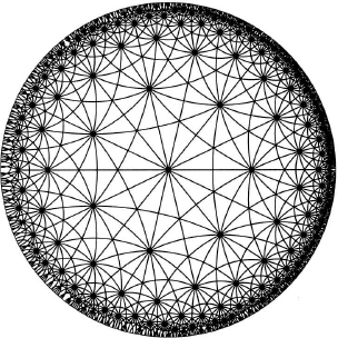
This is the (infinite) group of symmetries of a tiling of the hyperbolic plane with triangles whose angles are π/2, π/3, and π/7. This tiling is shown in Figure 5.4.
Figure 5.4 A triangle tiling of the hyperbolic plane.
EXERCISES
![]()
![]()
Notes
Richard Hamming (1915–1998) developed the Hamming codes in 1947 at Bell Telephone Laboratories in order to solve the problem of glitches in running computer programs. Marcel Golay (1902–1989) did much of the same work independently at the Signal Corps Engineering Laboratories. For a history of their achievements the reader is referred to [27]. Today, error-correcting codes are used in the design of compact discs (CDs), satellite communications, ISBN numbers, and bar code scanners. Error-correcting codes are an important part of the science of information theory introduced by Claude Shannon (1916–2001) in 1941 (also at Bell Labs). The main ideas of information theory are that an information source contains a certain amount of uncertainty (entropy) and that entropy determines the accuracy and amount of information that can be sent over a communication channel. In a memoryless source of English characters, for example, the entropy is thought to be about 4.03 bits (each revealed character conveys about 4.03 bits of information). As a baseline comparison, the entropy of a memoryless source of 27 equally likely symbols (26 letters and a space) is approximately 4.76 bits. (By the way, in a popular word-making board game the distribution of letter tiles gives an entropy value of about 4.32 bits.) However, if knowledge of the English language is used to predict the likelihood of future characters (the source has a memory), then the entropy is believed to be between 0.6 and 1.3 bits. Knowledge of the information structure of a language is useful in the design of machines that translate the spoken word into written text (continuous speech recognition).
A linear code has a generating matrix. The (7, 16, 3) Hamming code, as constructed in this chapter, is generated by the 7 × 4 matrix
The code is the range of the corresponding linear transformation, the set of vectors Gv ![]() F7, where v
F7, where v ![]() F4.
F4.
For a detailed introduction to error-correcting codes, a good source is [22].
1 In Fano’s geometry, what we call the Fano Configuration was specifically excluded.