CHAPTER 6
COMBINATORIAL DESIGNS
The Fano Configuration FC is the simplest nontrivial example of many types of combinatorial configurations, including t-designs, Steiner systems, block designs, and projective planes. We next explore these designs and investigate their interconnections, paving the way for the construction of the Golay code G23, the only perfect binary code capable of correcting more than one error, and Leech’s remarkable 24-dimensional lattice.
6.1 t-designs
A t-(v, k, λ) design (or t-design) consists of a v-set S and a collection C of k-subsets of S, with the property that every t-subset of S is contained in exactly λ members of C. The elements of S are called points and the elements of C are called blocks.
A t-design is nontrivial if 0 < t < k < v and not every k-subset of S is a block.
 EXAMPLE 6.1
The lines 246, 167, 145, 257, 123, 347, and 356 of FC are the blocks of a 2-(7, 3, 1) design with S = {1,…,7}.
EXAMPLE 6.2
The complement FC’ of FC has the same set of vertices as FC. Its lines are the complements of the lines of FC: 1357, 2345, 2367, 1346, 4567, 1256, 1247. It is easy to verify that the lines of FC’ constitute the blocks of a 2-(7, 4, 2) design.
EXAMPLE 6.3
The following sets are the blocks of a 3-(8, 4, 1) design:
![]()
These blocks are of two types: (1) the lines of FC’ and (2) the lines of FC joined to a new element 8. The derived design obtained by removing any point and all the sets not incident with it is equivalent to FC. Conversely, we call the 3−(8, 4, 1) design an extension of FC.
EXAMPLE 6.4
A graph with p vertices and q edges is a 0-(p, 2, q) design. An r-regular graph is a 1-(p, 2, r) design. An r-regular k-uniform hypergraph is a 1-(p, k, r) design.
We say that two t-designs are equivalent if they can be made the same by relabeling their underlying sets. Each of the nontrivial designs above is unique up to this equivalence. One reason for the uniqueness is that many parameters of a design are determined by the following theorem.
Parameter theorem. Given a t-(v, k, λ) design with point set S and block set C and 0 ≤ i ≤ t, there exists a constant λi such that every i-set of S lies in exactly λi elements of C. Therefore, the design is an i-(v, k, λi) design. Furthermore, λi satisfies ![]() .
.
Proof. Let X be a fixed subset of S with |X| = i, and consider the ordered pairs (T, K) with |T| = t, K ![]() C and X
C and X ![]() T
T ![]() K. As in the proof of Burnside’s lemma, we count the ordered pairs in two ways (from the perspective of each coordinate) to obtain
K. As in the proof of Burnside’s lemma, we count the ordered pairs in two ways (from the perspective of each coordinate) to obtain ![]() , a relation independent of X.
, a relation independent of X.
We solve the parameter equation for λi:
(6.1) 
Putting in the value i = 0, we obtain the number b of blocks in C:
Putting in the value i = 1, we obtain the number r of times each element of S occurs in a block:
The reader should verify the formulas for b and r in the above examples.
An S(t, k, v) Steiner system is a t-design with λ = 1. Later, we construct the Golay code G23 via a related code that contains an S(5, 8, 24) Steiner system. No Steiner system is known with t > 5. The only known Steiner systems with t = 5 are S(5, 6, 12), S(5, 6, 24), (5, 6, 36), S(5, 6, 48), S(5, 6, 72), S(5, 6, 84), S(5, 6, 108), S(5, 6, 132), S(5, 6, 168), S(5, 6, 244), S(5, 7, 28), and S(5, 8, 24) designs, and the only known Steiner systems with t = 4 are derived from these designs.
Open problem. Determine whether there is a Steiner system with t > 5.
A Steiner triple system is a Steiner system with k = 3.
EXAMPLE 6.5
FC is a S(2, 3, 7) Steiner triple system.
EXAMPLE 6.6
An S(2, 3, 9) Steiner triple system is given by the set of blocks
![]()
This Steiner system is equivalent to the set of nonideal points and lines of the projective plane of order 3.
EXAMPLE 6.7
Show that the weight 3 codewords of the Hamming code of length 15 form a Steiner triple system. What are its parameters?
EXAMPLE 6.8
The 81 cards of the SET® game are the points of an S(2, 3, 81) Steiner triple system. The blocks are the 1080 possible sets. Each block contains three points and each point is contained in exactly 40 blocks.
We can define further parameters for a t-(v, k, λ) design.
Double-parameter theorem. Given a t-(v, k, λ) design with points S and blocks C, and i and j nonnegative integers satisfying i + j ≤ t, there exists a constant λij such that the number of blocks which contain all the elements of any fixed i-set of S and omit all the elements of any fixed j-set of S (the i-set having no elements in common with the j-set) is exactly λij. Furthermore, λij satisfies
![]()
Proof. From the parameter theorem and the inclusion–exclusion principle, we obtain
It follows that
EXAMPLE 6.9
Recall that FC is a 2-(7, 3, 1) design. Applying the double-parameter theorem, we determine the constants λ00 = 7, λ10 = 3, λ01 = 4, λ20 = 1, λ11 = 2, λ02 = 2. For example, the relation λ11 = 2 says that, given any points x and y of FC, there are precisely two lines which contain x and omit y.
EXERCISES
6.2 Block designs
A balanced incomplete block design (BIBD) is a nontrivial 2-(v, k, λ) design. The parameter theorem shows that there is a number r such that each element of the set S occurs in exactly r blocks. Letting v = |S|, we rephrase the definition of balanced incomplete block design. A (v, b, r, k, λ) BIBD is a family C of b subsets (blocks or lines or edges) of a set S of v elements (points or vertices) such that:
EXAMPLE 6.10
FC is a (7, 7, 3, 3, 1) BIBD. FC′ is a (7, 7, 4, 4, 2) BIBD. The S(2, 3, 9) Steiner system is a (9, 12, 4, 3, 1) BIBD.
Parameter theorem for block designs. In a (v, b, r, k, λ) BIBD, bk = vr and r(k – 1) = λ(v – 1).
Proof. These relations follow from the parameter theorem for t-designs upon letting t = 2. The first result is obtained by dividing the relation (6.2) by the relation (6.3). The second result is immediate from (6.3).
The relations of the theorem can be proved without using the parameter theorem. To prove the first relation, note that the total number of incidences between vertices and blocks is bk (from the point of view of the blocks) and also vr (from the point of view of the vertices). Therefore bk = vr. To prove the second relation, note that the number of times a particular element occurs in pairs with other elements is r(k – 1). But it is also λ(v – 1), the number of elements with which the particular element may be paired multiplied by the number of times each pair occurs. Therefore r(k – 1) = λ(v – 1).
The incidence relation between blocks and vertices can be displayed in an incidence matrix A = [aij]b × v. We choose orderings of the points and the blocks and let aij = 1 if the jth point is an element of the ith block and aij = 0 otherwise. For instance, the points 1,…,7 and the blocks 246, 167, 145, 257, 123, 347, and 356 of FC are represented by the incidence matrix
Theorem. For any (v, b, r, k, λ) BIBD:
(6.4) ![]()
Proof. From the block size and balance condition of a BIBD, it follows that
(6.5) 
Subtracting the first row from the others, then replacing the first column with the sum of all the columns, we obtain
Fisher’s inequality. In any BIBD, b ≥ v.
Proof. Let A be an incidence matrix of the (v, b, r, k, λ) BIBD. Thus, A is a matrix of dimensions b × v. Let I be the v × v identity matrix and J the v × v all-1′s matrix. From the previous theorem it follows that AtA = λJ + (r – λ)I and det AtA = rk(r – λ)v−1. The relation r(k – 1) = λ(v – 1) implies that r > λ, which means that det(AtA) ≠ 0. Hence, v = rank(AtA) ≤ min{v, b} ≤ b.
The extreme case v = b gives rise to an interesting subclass of block designs. A (v, k, λ) square block design (SBD) is a (v, b, r, k, λ) BIBD in which v = b (and hence also k = r). Square block designs are usually called “symmetric block designs,” but this is probably not the best term for them as their incidence matrices are not symmetric. We believe that the term “square block design” is a better choice. Note that in a (v, k, λ) SBD we have k(k – 1) = λ(v – 1).
EXAMPLE 6.11
FC is a (7, 3, 1) SBD and FC’ is a (7, 4, 2) SBD.
Theorem. The incidence matrix A of a (v, k, λ) SBD is normal: AtA = AAt. Thus, any two distinct blocks intersect in exactly λ elements.
Proof. We have AtA = (k – λ)I + λJ. Because det(AtA) ≠ 0, it follows that det A ≠ 0, so A−1 exists. Therefore
![]()
Also, JA = kJ implies that JA−1 = k−1 J. Hence AAt = (k – λ)I + λJ. An interpretation of this matrix product yields the desired intersection property.
If A is the incidence matrix of an SBD, then (det A)2 = k2 (k – λ)v−1, and so det A = k(k – λ)(v−1)/2. It follows that if v is even, then k – λ is a perfect square. This is the first part of the Bruck–Chowla–Ryser theorem, stated below. For a proof of the second part, see [12].
Bruck–Chowla–Ryser theorem (1949). Suppose that a (v, k, λ) SBD exists. Then the following two statements hold:
![]()
has a solution in integers x, y, and z, not all zero.
EXAMPLE 6.12
There is no (22, 7, 2) SBD, since k – λ = 5, which is not a perfect square.
Let D be a BIBD. The complement D’ of D is obtained by switching 0 and 1 in an incidence matrix of D. It is easy to check that the complement of a (v, b, r, k, λ) BIBD is a (v, b, b – r, v – k, b – 2r + λ) BIBD. Specifically, the complement of a (v, k, λ) SBD is a (v, v – k, v – 2k + λ) SBD.
EXAMPLE 6.13
The S(2, 3, 9) Steiner system is a (9, 12, 4, 3, 1) BIBD whose complement is a (9, 12, 8, 6, 5) BIBD.
If p ![]() 3 (mod 4), then we can construct a
3 (mod 4), then we can construct a ![]() square design via the set Rp of quadratic residues modulo p. If p is any prime greater than 2, then the map f:
square design via the set Rp of quadratic residues modulo p. If p is any prime greater than 2, then the map f: ![]() → Rp with f(x) = x2 is an epimorphism with kernel { –1, 1}, from which it follows by the first homomorphism theorem for groups that |Rp| = (p – 1)/2. Let Np be the set of quadratic nonresidues modulo p, so that |Np| = (p – 1)/2. The Legendre symbol (x / p) is defined as
→ Rp with f(x) = x2 is an epimorphism with kernel { –1, 1}, from which it follows by the first homomorphism theorem for groups that |Rp| = (p – 1)/2. Let Np be the set of quadratic nonresidues modulo p, so that |Np| = (p – 1)/2. The Legendre symbol (x / p) is defined as
(6.6) 
Because |Rp| = |Np|, we have Σ(x/p) = 0 for any sum over a complete residue system modulo p.
Assuming that p ![]() 3 (mod 4), let A be the p × p circulant binary matrix whose first row is the characteristic vector of Rp ∪ {0} and whose other rows are successive one unit shifts to the right of the first row. We claim that A is the incidence matrix of a
3 (mod 4), let A be the p × p circulant binary matrix whose first row is the characteristic vector of Rp ∪ {0} and whose other rows are successive one unit shifts to the right of the first row. We claim that A is the incidence matrix of a ![]() SBD. Evidently, v = b = p and k = r =
SBD. Evidently, v = b = p and k = r = ![]() . We only need to check that the dot product of any two distinct rows is
. We only need to check that the dot product of any two distinct rows is ![]() . The dot product of two rows which differ by a shift of j units to the right is
. The dot product of two rows which differ by a shift of j units to the right is
![]()
where S is a complete residue system modulo p except for the values 0 and −j. Since p is congruent to 3 modulo 4, it follows that –1 is a quadratic nonresidue modulo p. Therefore, exactly one of j and –j is a quadratic residue and the other is a quadratic nonresidue. Letting x−1 be the multiplicative inverse of x, we have
Because x−1 takes all values except 0 and −j−1, it follows that 1 + jx−1 takes all values except 1 and 0. Therefore
![]()
and
![]()
For example, with p = 7, the construction furnishes a (7, 4, 2) design equivalent to FC′.
This construction produces square designs with large values of λ. Such designs are equivalent to Hadamard designs. At the opposite extreme, the next section deals with λ = 1 designs, which are called projective planes.
EXERCISES
6.3 Projective planes
In a (v, k, λ) SBD, suppose that λ = 1, and set n = k – 1. Then from the relation k(k – 1) = λ(v – 1), we have v = n2 + n + 1. Such a design is called a finite projective plane πn of order n. Thus, a πn is an (n2 + n + 1, n + 1, 1) SBD. The elements of πn are called points and the blocks are called lines. As a square design, a finite projective plane of order n has the following properties:
As we have seen with FC, these properties occur in pairs called duals properties. If the words “point” and “line” are interchanged, each property is transformed into its dual property.
EXAMPLE 6.14 A projective plane of order 2
FC is a projective plane of order 2.
Another description of projective planes comes from linear algebra. For FC, let F = {0, 1} be the two-element field, and let V = F3 = {(x, y, z) : x, y, z ![]() F}, the three-dimensional vector space over F. The points of the projective plane are the seven 1-dimensional subspaces of V, and the lines are the seven 2-dimensional subspaces of V. The reader can check that the above six properties hold.
F}, the three-dimensional vector space over F. The points of the projective plane are the seven 1-dimensional subspaces of V, and the lines are the seven 2-dimensional subspaces of V. The reader can check that the above six properties hold.
Theorem. A projective plane πn exists for every prime power n.
Proof. Let F = GF(n), the Galois field of order n. Let the set of points of the plane be
![]()
The points i ![]() F are called ideal points. The point ∞ is called the point at infinity. The lines are
F are called ideal points. The point ∞ is called the point at infinity. The lines are
The line l∞ is called the line at infinity. These n2 + n + 1 points and n2 + n + 1 lines constitute a πn. We need only check that the conditions for a (n2 + n + 1, n2 + n + 1, n + 1, n + 1, 1) BIBD are satisfied. Each point (i, j) lies on exactly n + 1 lines, namely, the lines lm,j – mi, where m ![]() F, and li. The reader should check that the ideal points and the point at infinity each lie on n + 1 lines. That each line contains n + 1 points can be seen from the definitions. We leave it to the reader to check that each pair of points determines exactly one line.
F, and li. The reader should check that the ideal points and the point at infinity each lie on n + 1 lines. That each line contains n + 1 points can be seen from the definitions. We leave it to the reader to check that each pair of points determines exactly one line.
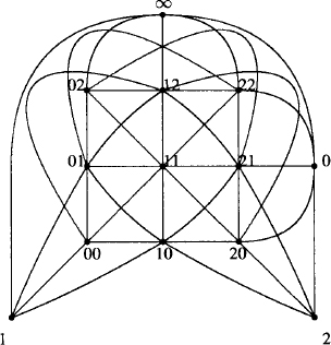
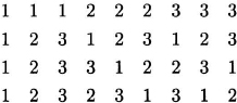
EXAMPLE 6.15 A projective plane of order 3
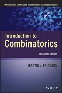
Let us use the description in the above proof to construct a projective plane of order 3 (Figure 6.1). The appropriate base field is F = GF(3), whose elements are 0, 1, 2. The 13 points are (i, j), with 0 ≤ i, j ≤ 2, which constitute the square array of the figure, and the ideal points i, with 0 ≤ i ≤ 2, and ∞, which are placed to the side. The lines are lm,b, where 0 ≤ m, b ≤ 2; lk, where 0 ≤ k ≤ 2; and l∞.
Figure 6.1 A projective plane of order 3.
By the Bruck–Chowla–Ryser theorem, if there is a projective plane of order n and if n ![]() 1, 2 (mod 4), then there is a solution in integers to the equation
1, 2 (mod 4), then there is a solution in integers to the equation
![]()
It follows that
![]()
i.e., n is expressible as the sum of the squares of two rational numbers. From elementary number theory, it follows that n is the sum of two squares of integers. Hence, there is no projective plane of order 6 or 14. However, 10 = 32 + 12, so the Bruck–Chowla–Ryser theorem does not rule out the possibility of a projective plane of order 10. In 1988 C. W. H. Lam, leading a team, used a computer to prove the nonexistence of a projective plane of order 10. See C. W. H. Lam, “The search for a finite projective plane of order 10,” American Mathematical Monthly, 98 (1991), pp. 305–318.
As we showed, there exists a projective plane of every prime power order. No projective plane of order not a prime power is known to exist, and it is conjectured that there is none.
Open problem. Construct a projective plane of order 12 or show that none exists.
A finite affine plane π’n is a projective plane of order n without the ideal points and the line at infinity. A π′n is an (n2, n2 + n, n + 1, n, 1) BIBD. For example, a π′3 is a (9, 12, 4, 3, 1) BIBD, which we have already seen is an S(2, 3, 9) Steiner system. In general, a π′n is an S(2, n, n2). A projective plane of order n exists if and only if there exists an affine plane of order n. See [20].
EXERCISES
6.4 Latin squares
A Latin square L of order n is an n × n array [L(i, j)] in which each row and each column contains all the elements of Nn. An r × n Latin rectangle consists of the first r rows of a Latin square of order n.
It is easy to create a Latin square of any order, as in the next example.
EXAMPLE 6.16 A Latin square of order 3
To create a Latin square of order 3, take the first row to be 1, 2, 3, and sucessive rows to be shifts of the first row.

EXAMPLE 6.17
The Cayley table of a finite group G with elements g1,…,gn yields a Latin square L of order n. Let the (i, j) entry of L be k, where gigj = gk. For instance, G = Z2 × Z2, with elements (0, 0), (0, 1), (1, 0), (1, 1), yields the Latin square

Not all Latin squares come from groups. However, Latin squares are equivalent to the multiplication tables of primitive algebraic structures called quasigroups. We record some interesting definitions. A groupoid is a nonempty set S and a binary operation * defined on S. A semigroup is a groupoid in which * is an associative operation. A monoid is a semigroup containing a two-sided identity element e (x * e = e * x = x for all x). A group is a monoid in which every element x in S has a two-sided inverse x−1 ![]() . A quasigroup is a groupoid such that given a, b
. A quasigroup is a groupoid such that given a, b ![]() S there exist unique x, y with a * x = b and y * a = b. A loop is a quasigroup containing a two-sided identity e. The literature abounds with examples of these algebraic structures. For instance, given any S(2, 3, n) Steiner triple system S we may define a quasigroup whose elements are members of S by setting, for a and b distinct, a * b = c, where c is the unique element in a triple with a and b, and setting a * a = a. By adding an identity element 1 and properly extending the definition of multiplication we may turn this quasigroup into a loop. Another example of a loop is the famous Cayley loop of order 16. To see some other loops the reader should consult [7].
S there exist unique x, y with a * x = b and y * a = b. A loop is a quasigroup containing a two-sided identity e. The literature abounds with examples of these algebraic structures. For instance, given any S(2, 3, n) Steiner triple system S we may define a quasigroup whose elements are members of S by setting, for a and b distinct, a * b = c, where c is the unique element in a triple with a and b, and setting a * a = a. By adding an identity element 1 and properly extending the definition of multiplication we may turn this quasigroup into a loop. Another example of a loop is the famous Cayley loop of order 16. To see some other loops the reader should consult [7].
Suppose that we have a quasigroup with n elements, g1,…,gn. By definition, each row and each column of its multiplication table is a permutation of the n elements. Therefore, replacing g1,…,gn by the numbers 1,…,n results in a Latin square of order n. Conversely, any Latin square of order n is the multiplication table of a quasigroup of order n.
Two Latin squares L1 and L2 are equivalent if L1 can be transformed into L2 by the following operations:
It is an open problem to determine an asymptotic formula for the number L(n) of Latin squares of order n (equivalently, the number of quasigroups of order n) and the number L* (n) of inequivalent Latin squares of order n. However, the following existence theorem allows us to formulate a lower bound for L(n).
Hall’s marriage theorem (1935). Let S1,…,Sn be finite sets. There exist distinct si ![]() Si (for each i) if and only if the following condition holds for each k with 1 ≤ k ≤ n: the union of any k of the Si contains at least k elements.
Si (for each i) if and only if the following condition holds for each k with 1 ≤ k ≤ n: the union of any k of the Si contains at least k elements.
The set {si} is called a system of distinct representatives (SDR) for the Si. If Si is a list of men whom woman i would like to marry, then an SDR is a feasible set of marriages; hence the title of the theorem.
Proof. The necessity of the conditions is obvious. We must prove that the conditions are sufficient. Certainly, there is a representative for the first set. Assume that distinct representatives exist for the first k of the sets. We will show that an SDR can be found for k + 1 sets. Let T1 be a set which has no representative assigned to it yet. If there is an element of T1 not already occurring as a representative of one of the other k sets, then we are done. Otherwise, note that T1 has at least one element, say t1, and suppose that t1 represents T2. By hypothesis, T1 ∪ T2 contains at least one element other than t1, say t2. If t2 is not already a representative, then stop. If t2 represents a set T3, then find t3 ![]() T1 ∪ T2 ∪ T3. Continuing in this manner, we find a collection {ti} such that ti
T1 ∪ T2 ∪ T3. Continuing in this manner, we find a collection {ti} such that ti ![]() T1 ∪ · · · ∪ Ti and ti represents Ti+1 (for i < a), and ta is not a representative yet. Now we change some representatives by pairing ta with a set Ta′ where a ≤ a′. This process continues until T1 is paired with a representative. These new pairings, together with the unchanged pairings, constitute an SDR for k + 1 sets.
T1 ∪ · · · ∪ Ti and ti represents Ti+1 (for i < a), and ta is not a representative yet. Now we change some representatives by pairing ta with a set Ta′ where a ≤ a′. This process continues until T1 is paired with a representative. These new pairings, together with the unchanged pairings, constitute an SDR for k + 1 sets.
The following corollary is proved in [12].
Corollary. If S1,…,Sn are sets possessing an SDR, and if the smallest set has size t < n, then the Si possess at least t! SDRs.
Lower bound for the number of Latin squares. L(n) ≥ n!(n – 1)! … 2!1!.
Proof. We will show that for each r, where 1 ≤ r ≤ n – 1, an r × n Latin rectangle may be extended to an (r + 1) × n Latin rectangle in at least (n – r)! ways. Given an r × n Latin rectangle, let Si be the set of numbers not yet used in column i. Clearly, an SDR could be used as the (r + 1)st row of the Latin square. Now, each element m, with 1 ≤ m ≤ n, has occurred in r rows and hence in r columns of the Latin rectangle thus far. Therefore, each element occurs in exactly n – r of the Si. For each k, the union of k of the Si contains k(n – r) elements (counting repetitions). As each element occurs in at most n – r of these Si, the union must contain at least k elements, and the criterion in Hall’s theorem is satisfied. Hence, there is an SDR for the Si.
Because each Si has size n – r, the corollary guarantees the existence of at least (n – r)! SDRs. The inequality on L(n) is established by applying the above estimate as each successive row is added to the Latin square.
By a permutation of its rows and columns, any Latin square may be written with 1,…,n as its first row and first column. Such a Latin square is said to be standardized. If L′(n) is the number of inequivalent standardized Latin squares of order n, then L(n) = n!(n – 1)!L′(n). Table 6.1 gives the values of L′(n) for 1 ≤ n ≤ 7.
Table 6.1 The number of standardized Latin squares.

Open problem. Find a formula for L′(n).
EXERCISES
6.5 MOLS and OODs
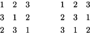
Two Latin squares L1 = [L1(i, j)] and L2 = [L2(i, j)] of order n are orthogonal if, for every (a, b) ![]() Nn × Nn, there is an ordered pair (i, j) with (L1(i, j), L2(i, j)) = (a, b). In other words, the ordered pairs (L1(i, j), L2(i, j)) take each of the n2 values in Nn × Nn exactly once. The two Latin squares of Figure 6.2 are orthogonal.
Nn × Nn, there is an ordered pair (i, j) with (L1(i, j), L2(i, j)) = (a, b). In other words, the ordered pairs (L1(i, j), L2(i, j)) take each of the n2 values in Nn × Nn exactly once. The two Latin squares of Figure 6.2 are orthogonal.
Figure 6.2 Two orthogonal Latin squares of order 3.
A set of mutually orthogonal Latin squares, or MOLS, is a set in which every pair is orthogonal. MOLS are also called pairwise orthogonal Latin squares. We define m(n) to be the maximum possible number of MOLS of order n. Leonhard Euler (1707–1783) introduced the ideas of Latin squares and MOLS in 1782 when he asked whether there are two MOLS of order 6. He believed the answer is no and therefore conjectured that m(6) = 1. This was proved by G. Tarry in 1900. Euler also conjectured that m(n) = 1 whenever n ![]() 2 (mod 4), but it was shown in 1960 by R. C. Bose, E. T. Parker, and S. S. Shrikhande that m(n) ≥ 2 except when n = 1, 2, or 6. For example, there are two MOLS of order 10. However, it is not known whether there are three MOLS of order 10.
2 (mod 4), but it was shown in 1960 by R. C. Bose, E. T. Parker, and S. S. Shrikhande that m(n) ≥ 2 except when n = 1, 2, or 6. For example, there are two MOLS of order 10. However, it is not known whether there are three MOLS of order 10.
Theorem. For all n ≥ 2, we have m(n) ≥ n – 1.
Proof. Suppose that there is a set of n MOLS of order n. By a permutation of symbols, the first row of each Latin square can be changed to 1,…,n, and permuting symbols clearly does not disturb orthogonality. Now, by the pigeonhole principle, since none of the (2, 1) entries of the n MOLS can equal 1, some two Latin squares have (2, 1) entry equal to i, with 2 ≤ i ≤ n. But these Latin squares are not orthogonal because the ordered pair (i, i) occurs twice in the list of ordered pairs of entries.
When n = pk for a prime p, we can construct n – 1 MOLS of order n. Suppose that F is the field GF(pk), and let F = {0 = f0,…,fn–1}. For each m, where 1 ≤ m ≤ n – 1, define the Latin square Lm = [Lm(i, j)]n × n, where 0 ≤ i, j ≤ n – 1, by Lm(i, j) = fmfi + fj. It is a simple matter to check that each Lm is a Latin square. To check the orthogonality condition, observe that ![]() =
= ![]() implies that fi = fk and fj = fl, so all the ordered pairs are distinct.
implies that fi = fk and fj = fl, so all the ordered pairs are distinct.
For example, starting with the three-element field {0, 1, 2}, we produce the two MOLS
or
(two orthogonal Latin squares equivalent to those in Figure 6.2).
We have described how a projective plane of order n can be constructed from the field GF(n). The above argument shows that n – 1 MOLS of order n can be constructed from GF(n). In fact, a projective plane of order n is equivalent to a set of n – 1 MOLS of order n.
Theorem. A set of n – 1 MOLS of order n is equivalent to a projective plane of order n.
Proof. Suppose that we are given n – 1 MOLS: L1,…,Ln−1. Let
![]()
and define
We leave it to the reader to check that the incidence matrix for the set of points S and the lines l∞,k, l0,k, lx,y, l∞ is an (n2 + n + 1, n + 1, 1) SBD.
Reversing the above construction completes the equivalence.
The reader may find it instructive to apply the construction technique to the two MOLS of Figure 6.2 to construct a projective plane of order 3. It will be equivalent to the one of Figure 6.1.
Let us extend the definition of orthogonality to any two square matrices (not necessarily Latin squares). We say that two n × n matrices A and B with entries from Nn are orthogonal if the ordered pairs (A(i, j), B(i, j)) take each of the n2 values in Nn × Nn exactly once. Observe that the matrices
are orthogonal. With this generalized definition of orthogonality, we can give an elegant characterization of Latin squares: an n × n matrix is an order n Latin square if and only if it is orthogonal to both R and C. Thus, any k MOLS of order n are part of a family of k + 2 mutually orthogonal matrices. Conversely, any k + 2 mutually orthogonal n × matrices may be transformed into R, C, and k MOLS of order n. For if a matrix M is orthogonal to another matrix, then M contains each of the numbers 1,…,n exactly n times. Therefore, choosing two matrices M and N from the set of k + 2 orthogonal matrices, we may transform M into R and N into C by a simultaneous permutation of the entries of all the matrices. Discarding R and C, we are left with k MOLS of order n.
This characterization replaces the notion of Latinicity with the more essential notion of orthogonality. Accordingly, we define an ordered orthogonal design of order n and depth s (an (n, s) OOD) to be an s × n2 matrix (mij) with entries 1,…,n such that every two rows are orthogonal. That is, for every pair of rows u and v, every ordered pair (a, b) with 1 ≤ a, b ≤ n occurs exactly once among the ordered pairs (mui, mvi). For example, Figure 6.3 shows a (3, 4) OOD derived from the two Latin squares of order 3 in Figure 6.2. An OOD is also called an OA (orthogonal array).
Figure 6.3 A (3,4) OOD.
The design inherent in the theorem can be produced directly from an (n, n + 1) OOD. In general, an OOD-net based on an (n, s) OOD is a collection of m points corresponding to the columns of the OOD and s pencils of parallel lines, where point xj is on line y of the ith pencil if the (i, j) entry of the matrix is y. The OOD-net of an (n, n + 1) OOD is an affine plane of order n which may be extended to a projective plane of order n by the addition of one ideal point for each row of the OOD and an ideal line.
In summary, we have shown the equivalence of the following discrete configurations:
Open problem. Determine the values of n for which these structures exist.
A possible conjecture consistent with what is known is that these structures exist if and only if n is a prime power.
EXERCISES
6.6 Hadamard matrices
In 1893 Jacques Hadamard considered a basic problem about the maximum absolute value of the determinant of a matrix with bounded entries.
Hadamard’s theorem (1893). Suppose A = [aij] is matrix of order m with –1 ≤ aij ≤ 1 for all i and j. Then |det A| ≤ mm/2, and the upper bound is obtained if and only if aij = ±1 for all i and j and AAt = mI.
Proof. The rows of A are vectors in Rn of length at most m1/2, and they span a parallelepiped of volume |det A|. This volume is clearly maximized when the vectors are mutually orthogonal and of maximum possible length, and in this case the volume is the product of the lengths, mm/2.
A matrix A = [aij]m × m with aij = ±1 and AAt = mI is called a Hadamard matrix of order m. The condition AAt = mI means that the dot product of any two distinct rows of A is zero. (The same is true for columns, as AtA = A−1 (AAt)A = A−1(mI)A = mI.) Therefore, without regard to the volume argument given in the proof above, if A is a Hadamard matrix of order m, then mm = det AAt = (det A)2, which implies that |det A| = mm/2.
Notice that the theorem does not address the question of the maximum value of |det A| when there is no Hadamard matrix of order m. However, |det A| does attain a maximum, as it is a continuous function defined on a compact set (the cube [ –1, 1]m2). Furthermore, because det A is a linear function of each entry aij (i.e., a straight line), the function y = |det A| is concave upward and therefore the maximum of |det A| occurs when each aij = –1 or 1. The maximum determinant may also occur for other matrices, in case the coefficient of the first-order term in the linear equation just described is 0. For example,
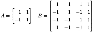
The Kronecker product A ⊗ B of two square matrices A = [aij]m1 × m1 and B = [bij]m2 × m2 is the square matrix A ⊗ B = [aijB]m1 m2 × m1m2. The Kronecker product produces larger Hadamard matrices from smaller ones. For example, Figure 6.4 shows Hadamard matrices A and B of orders 2 and 4, respectively, with B = A ⊗ A.
Figure 6.4 Hadamard matrices of orders 2 and 4.
If H is a Hadamard matrix, then so is

Theorem. There exists a Hadamard matrix of order m = 2k, where k is any positive integer.
If A is a Hadamard matrix, then any permutation of the rows or columns of A is a Hadamard matrix. Also, any row or column of A may be multiplied by –1 with the result still a Hadamard matrix. With these operations it is possible to alter any Hadamard matrix so that its first row and first column consist of all 1′s. Such a Hadamard matrix is said to be normalized.
Theorem. If A is a Hadamard matrix of order m > 2, then m is a multiple of 4.
Proof. Normalize A and permute its columns so that its first three rows look like this:
(The variables a, b, c, d are to be determined.) Four equations are immediate from the definition of a Hadamard matrix:
Adding the equations yields 4a = m, from which it follows that a = b = c = d = m/4. Therefore, m is a multiple of 4, and furthermore we have found that any row after the first has m/2 1′s and m/2 –1′s, and any two rows (not including the first) have 1′s together in m/4 columns.
It is conjectured that the condition of the theorem is sufficient as well as necessary.
Conjecture. There exists a Hadamard matrix of every order a multiple of 4.
The smallest order for which the existence of a Hadamard matrix is not certain is 668.
Open problem. Determine whether there is a Hadamard matrix of order 668.
Theorem. Let H be a normalized Hadamard matrix of order 4n ≥ 8. Deleting the first row and column of H and changing each –1 to a 0 results in an incidence matrix of a (4n – 1, 2n – 1, n – 1) SBD. Conversely, starting with an incidence matrix of a (4n – 1, 2n – 1, n – 1) SBD, changing each 0 to –1, and adding a first row and first column of all 1′s, yields a normalized Hadamard matrix of order 4n.
Proof. Let X be the submatrix of H formed by deleting its first row and column. The Hadamard conditions imply that XJ = JX = –J and XXt = 4nI – J. When each –1 is switched to 0 a new matrix Y = ![]() (X + J) results. We check that Y is the incidence matrix of a (4n – 1, 2n – 1, n – 1) SBD: JY = YJ =
(X + J) results. We check that Y is the incidence matrix of a (4n – 1, 2n – 1, n – 1) SBD: JY = YJ = ![]() (–J + (4n – 1)J) = (2n – 1)J and YYt =
(–J + (4n – 1)J) = (2n – 1)J and YYt = ![]() (X + J)(Xt + J) = nI + (n –1)J. The proof of the reverse construction is similar.
(X + J)(Xt + J) = nI + (n –1)J. The proof of the reverse construction is similar.
EXAMPLE 6.18
The (7, 3, 1) SBD is equivalent to a Hadamard matrix of order 8.
A (4n – 1, 2n – 1, n – 1) SBD created this way is called a Hadamard design of order n. A 3-(4n, 2n, n – 1) design may be formed by taking complements of a Hadamard design H together with the blocks of H joined to a new point ∞.
Hadamard designs and projective planes are two extreme types of (v, k, λ) designs. For if a (v, k, λ) design exists, then
(6.7) ![]()
where n = k –λ. To prove this inequality, we let λ′ = v – 2k + λ. Then λ + λ′ = v – 2n and λλ′ = n(n – 1). The upper bound follows from the observation that λ′ ≥ 1, and the lower bound from the arithmetic mean–geometric mean inequality, (λ + λ′)2 ≥ 4λλ′. One can show that the upper bound is met if and only if the design is a projective plane of order n (or its complement) and the lower bound is met only for a Hadamard design of order n (or its complement).
Let H be a normalized Hadamard matrix of order m = 4n, with each –1 changed to 0, and let A be the code consisting of the rows of H and the binary complements of these rows. Clearly, A is a code of dimension 4n containing 8n codewords. We claim that the distance of A is 2n. We are guaranteed that any two rows of H disagree in exactly 2n places. Therefore, any two rows of the binary complementary matrix H′ disagree in 2n entries. Suppose that a ![]() H and b
H and b ![]() H′. If a = bc, then d(a, b) = m. If not, then d(a, b) equals the number of components in which a and bc agree, which is 2n. This (4n, 8n, 2n) code is called a Hadamard code. It is capable of detecting 2n – 1 errors and correcting n – 1 errors.
H′. If a = bc, then d(a, b) = m. If not, then d(a, b) equals the number of components in which a and bc agree, which is 2n. This (4n, 8n, 2n) code is called a Hadamard code. It is capable of detecting 2n – 1 errors and correcting n – 1 errors.
EXAMPLE 6.19
The (7, 3, 1) SBD yields an (8, 16, 4) code. We saw this code in Chapter 5.
EXAMPLE 6.20
From the complement of the quadratic residues construction for p = 11, we obtain the incidence matrix of an (11, 5, 2) SBD:
From Y we construct a normalized Hadamard matrix of order 12. Thus
We shall see in the next section that Y is one of the main ingredients in producing a perfect (23, 212, 7) code. Switching –1 back to 0, the rows of H and their complements constitute a (12, 24, 6) code which detects five errors and corrects two errors. The words of this code are listed below.
The families of codes we have encountered can be arranged on a continuum from good rate/bad distance to bad rate/good distance, as in Figure 6.5. At the left extreme is the code Fn, in which every vector is a codeword. The rate is 1, but the code is incapable of correcting any errors. At the right extreme is a code consisting of any vector v and its complement vc. Although this code has the highest possible distance, d = n, its rate is 1/n, the lowest possible. The family of Hamming codes are capable of correcting e = 1 error, and the rates tend to 1. Therefore, the Hamming codes converge to the left endpoint of the continuum. For the Hadamard codes,
Figure 6.5 The world of codes.

(6.8) ![]()
Since their rates converge to 0, the Hadamard codes converge to the right endpoint of the continuum.
The (23, 212, 7) Golay code G23, which we will construct in the next section, has rate 12/23 and corrects e = 3 errors.
We conclude the discussion of combinatorial designs by constructing three large, interesting, related configurations, namely, the (23, 212, 7) Golay code G23 (the only perfect multi-error-correcting binary code), the S(5, 8, 24) Steiner system (consisting of the weight 8 codewords of the extended Golay code G24), and Leech’s lattice ![]() (a 24-dimensional lattice obtained from G24 which generates a surprisingly dense sphere packing).
(a 24-dimensional lattice obtained from G24 which generates a surprisingly dense sphere packing).
EXERCISES
6.7 The Golay code and S(5, 8, 24)
We have indicated that the only feasible parameters for perfect binary codes with e > 1 are (90, 278, 5) and (23, 212, 7). An exercise calls for a proof that no (90, 278, 5) code exists. We will construct a (23, 212, 7) code called the Golay code, G23, which was discovered by Marcel Golay (1902–1989). It is a perfect 3-error correcting code with 212 words, sitting inside F23. As a bonus, we will find that certain words in the extended Golay code G24 constitute a Steiner system S(5, 8, 24).
Let M be an (11, 6, 3) SBD based on quadratic residues modulo 11. Let G be the 12 × 24 matrix
where I11 is the order 11 identity matrix.
The matrix G defines a linear transformation G: F12 → F24, with x ![]() xG. The (linear) code G24 is the image {xG : x
xG. The (linear) code G24 is the image {xG : x ![]() F12}. We call G a generating matrix for G24. It is easy to use a computer to produce the codewords of G24 and thereby verify that it is a (24, 212, 8) code. But we can do so without a computer as follows.
F12}. We call G a generating matrix for G24. It is easy to use a computer to produce the codewords of G24 and thereby verify that it is a (24, 212, 8) code. But we can do so without a computer as follows.
We leave it to the reader to use elementary row operations to reduce G to row echelon form and thus show that G has rank 12. It follows that G24 has parameters (24, 212, d), where d is to be determined. We proceed to find the weight distribution of G24.
Recall from Exercise 5.3 that if x and y are any two vectors of the same length, then w(x + y) = w(x) + w(y) – 2x · y.
If ri and rj are different rows of G, then ri · rj is even. This follows from the row dot product property of M.
Now we show that if x ![]() G24, then w(x) is a multiple of 4. Any codeword is a linear combination (over F) of the rows of G, so we can write x = r1 + r2 + · · · rn (with relabeling of rows). We use induction on n. If n = 1, then by inspection w(x) is a multiple of 4 (the last row has weight 12 and every other row has weight 8). Now if x = r1 + r2 + · · · + rn rn+1 then
G24, then w(x) is a multiple of 4. Any codeword is a linear combination (over F) of the rows of G, so we can write x = r1 + r2 + · · · rn (with relabeling of rows). We use induction on n. If n = 1, then by inspection w(x) is a multiple of 4 (the last row has weight 12 and every other row has weight 8). Now if x = r1 + r2 + · · · + rn rn+1 then
![]()
which, by remarks made earlier, is a multiple of 4. This completes the induction.
Therefore, the possible weights of words of G24 are 0, 4, 8, 12, 16, 20, 24. Clearly, 0 ![]() G24 and w(0) = 0. Also, r1 + r2 + · · · + r24 = (1,…,1), so there is a word of weight 24. It follows that the binary complement of any codeword is also a codeword and therefore the weight distribution of G24 is symmetric. This distribution, as we have found so far, is given by Table 6.2. The variables α, β, γ have yet to be determined.
G24 and w(0) = 0. Also, r1 + r2 + · · · + r24 = (1,…,1), so there is a word of weight 24. It follows that the binary complement of any codeword is also a codeword and therefore the weight distribution of G24 is symmetric. This distribution, as we have found so far, is given by Table 6.2. The variables α, β, γ have yet to be determined.
Table 6.2 The partially determined weight distribution of G24.
Suppose that x ![]() G24. Let L(x) be the left-hand string of length 12 of x and R(x) the right-hand string. We can now represent x as x = [L(x), R(x)]. We claim that [R(x), L(x)]
G24. Let L(x) be the left-hand string of length 12 of x and R(x) the right-hand string. We can now represent x as x = [L(x), R(x)]. We claim that [R(x), L(x)] ![]() G24; that is, G24 is invariant under the permutation of coordinates
G24; that is, G24 is invariant under the permutation of coordinates
![]()
We say that G24 is self-symmetric. Let v′ denote the vector obtained from v by switching the right and left halves. We leave it to the reader to show that for each row r of G, the vector r′ is a linear combination of the rows ri. It follows that G24 is invariant under τ, as every codeword of G24 is a sum of rows ri.
Next we observe that w(L(x)) is even whenever x ![]() G24, because the sum of k rows when k is even yields w(L(x)) = k and the sum when k is odd yields w(L(x)) = k + 1.
G24, because the sum of k rows when k is even yields w(L(x)) = k and the sum when k is odd yields w(L(x)) = k + 1.
Because w(L(x)) + w(R(x)) is a multiple of 4, it follows that w(R(x)) is always even.
Finally, we will show that d ≥ 8, from which it follows that d = 8, because the first row of G has weight 8. We need only show that no codeword has weight 4. If x has weight 4, then (w(L(x)), w(R(x))) = (0, 4), (4, 0), or (2, 2). If w(L(x)) = 0, then x must be r12, but then w(R(x)) = 8 > 4. Because G24 is self-symmetric, the (4, 0) case is ruled out also. For the (2, 2) case, we can sum any one or two of the first 11 rows of G and then add or not add the 12th row. In each case the resulting codeword has weight 6, not 2.
Therefore, G24 is a (24, 212, 8) code. Deleting any coordinate of G24 produces the Golay code G23, a code with parameters (23, 212, 7).
Theorem. The Golay code G23 is a (perfect) (23, 212, 7) code.
Let us complete the weight distribution table of G24. We know that G24 has no codewords of weight 4 or 20. How many words have weight 8? If w(x) = 8, then (w(L(x)), w(R(x))) equals (0, 8), (2, 6), (4, 4), (6, 2), or (8, 0). A glance at G shows that (0, 8) is impossible, and hence by self-symmetry (8, 0) is impossible. To obtain a weight partition (2, 6), we can add one or two rows of the first 11 rows of G and then add or not add the 12th row. There are ![]() +
+ ![]() = 132 possibilities. Likewise, there are 132 ways to obtain a codeword with weight partition (6, 2). To get a (4, 4) weight partition, we add either three or four rows of G. The number of choices is
= 132 possibilities. Likewise, there are 132 ways to obtain a codeword with weight partition (6, 2). To get a (4, 4) weight partition, we add either three or four rows of G. The number of choices is ![]() +
+ ![]() = 495. Altogether, the number of words of weight 8 in G24 is 132 + 132 + 495 = 759.
= 495. Altogether, the number of words of weight 8 in G24 is 132 + 132 + 495 = 759.
We display the complete weight distribution of G24 in Table 6.3.
Table 6.3 The weight distribution of G24.
We are now ready to find the Steiner system S(5, 8, 24) sitting inside G24. From the parameter theorem for S(5, 8, 24), we obtain λ5 = 1, λ4 = 5, λ3 = 21, λ2 = 77, λ1 = 253, and λ0 = 759. As λ0 is the number of blocks, it is clear that the words of weight 8 in G24 should form the blocks of S(5, 8, 24). Let S be the set of coordinates 1,…,24 and let C be the collection of sets of eight coordinates which equal 1 in codewords of weight 8 in G24. We need to check that the t = 5 and λ = 1 conditions are met. This means that every five-element subset of S is contained in exactly one block in C. Equivalently, every vector of weight 5 is covered by exactly one codeword of weight 8 in G24.
A vector v of weight 5 cannot be covered by two different codewords x and y of weight 8, or else w(x + y) ≤ 6, a contradiction.
Therefore, it remains to demonstrate that there are enough codewords of weight 8 to satisfy the λ = 1 condition. There are ![]() vectors of weight 5, and each of the 759 codewords of weight 8 covers
vectors of weight 5, and each of the 759 codewords of weight 8 covers ![]() of them. A simple calculation shows that
of them. A simple calculation shows that ![]() . Therefore, S and C make up the desired Steiner system S(5, 8, 24).
. Therefore, S and C make up the desired Steiner system S(5, 8, 24).
Theorem. The weight 8 codewords of G24 are an S(5, 8, 24) Steiner system.
EXERCISES
![]()
6.8 Lattices and sphere packings
An n-dimensional lattice ![]() is a subset of Rn such that:
is a subset of Rn such that:
We assume that ![]() contains a point other than the origin (hence
contains a point other than the origin (hence ![]() is infinite) and that
is infinite) and that ![]() is discrete, which means that
is discrete, which means that ![]() has a finite intersection with any compact subset of Rn.
has a finite intersection with any compact subset of Rn.
The Euclidean distance between two points x and y in Rn is
(6.9) ![]()
and the norm of x is
(6.10) ![]()
If ![]() is a discrete n-dimensional lattice containing a non-origin point x, then the Euclidean sphere
is a discrete n-dimensional lattice containing a non-origin point x, then the Euclidean sphere ![]() contains only finitely many points of
contains only finitely many points of ![]() . The minimum positive distance between 0 and a point in this intersection is the minimum distance of
. The minimum positive distance between 0 and a point in this intersection is the minimum distance of ![]() , denoted d(
, denoted d(![]() ). Two lattice points are neighbors if they are separated by this minimum distance. Because a lattice is clearly translation invariant, any base point determines the same minimum distance d(
). Two lattice points are neighbors if they are separated by this minimum distance. Because a lattice is clearly translation invariant, any base point determines the same minimum distance d(![]() ) to a neighbor. If spheres of radius
) to a neighbor. If spheres of radius ![]() d(
d(![]() ) are centered at each lattice point, these spheres touch only at their surfaces. Such a placement of spheres is called a lattice sphere packing of Rn.
) are centered at each lattice point, these spheres touch only at their surfaces. Such a placement of spheres is called a lattice sphere packing of Rn.
It is desirable to know how densely spheres may be packed in Rn via a lattice packing or otherwise. Related to this question is the computation of the maximum number of spheres touching a given sphere in a lattice packing. Specifically, let c(![]() ), the contact number of
), the contact number of ![]() , be the number of spheres of radius
, be the number of spheres of radius ![]() d(L) which touch the sphere centered at the origin. Equivalently, c(
d(L) which touch the sphere centered at the origin. Equivalently, c(![]() ) is the number of lattice points at distance d(
) is the number of lattice points at distance d(![]() ) from 0.
) from 0.
Figure 6.6 shows part of a two-dimensional lattice with distance 2 and contact number 4. This lattice is called (2Z)2, as it consists of all points in the plane with even integer coordinates. In general, the n-dimensional lattice (2Z)n consists of all points in Rn with even integer coordinates.
Figure 6.6 A lattice packing with contact number 4 and density ![]() 0.79.
0.79.
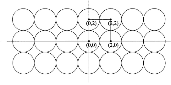
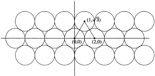
We can easily calculate the amount of the plane enclosed by the circles. Consider a square of area 4 whose vertices are four lattice points (as indicated in the figure). Such a square is called a fundamental region of the packing, as this region repeats periodically to give the complete pattern of the packing. Because the square contains four circular quadrants whose total area is π, we say that the density of the packing is π/4 ![]() 0.79. However, the densest possible packing in R2 is not based on the lattice (2Z)2, but on the triangular lattice T shown in Figure 6.7. The fundamental region of T is an equilateral triangle of side length 2 and area √3. As this triangle contains three sixths of a unit circle, the density of the packing is π/(2√3)
0.79. However, the densest possible packing in R2 is not based on the lattice (2Z)2, but on the triangular lattice T shown in Figure 6.7. The fundamental region of T is an equilateral triangle of side length 2 and area √3. As this triangle contains three sixths of a unit circle, the density of the packing is π/(2√3) ![]() = 0.90. The contact number, 6, is also greater for T than for (2Z)2. Because a unit sphere in the (2Z)n packing has two neighbors in each of n directions, this lattice has contact number 2n. We shall see that the contact number can be greatly improved in 24 dimensions.
= 0.90. The contact number, 6, is also greater for T than for (2Z)2. Because a unit sphere in the (2Z)n packing has two neighbors in each of n directions, this lattice has contact number 2n. We shall see that the contact number can be greatly improved in 24 dimensions.
Figure 6.7 A lattice packing with contact number 6 and density ![]() 0.90.
0.90.
Open problem. Find, for each k, the highest possible contact number of a lattice sphere packing in Rk.
EXERCISES
6.9 Leech’s lattice
In 1965 John Leech (1926–1992) proved that the extended Golay code G24 can be used to construct a 24-dimensional lattice with a remarkably high contact number. Leech’s lattice ![]() is defined as follows. For each codeword c = (c1,…,c24)
is defined as follows. For each codeword c = (c1,…,c24) ![]() G24 and each integer m, let
G24 and each integer m, let ![]() (c, m) be the set of integer 24-tuples (x1,…,x24) for which
(c, m) be the set of integer 24-tuples (x1,…,x24) for which
Leech’s lattice ![]() is the union of all the
is the union of all the ![]() (c, m).
(c, m).
We need to verify that ![]() is a lattice. Because the all-0 string is a codeword in G24, it follows that 0
is a lattice. Because the all-0 string is a codeword in G24, it follows that 0 ![]()
![]() (with m = 0). If x
(with m = 0). If x ![]()
![]() , then x
, then x ![]()
![]() (c, m) for some c
(c, m) for some c ![]() G24 and some integer m. It is easy to show that –x
G24 and some integer m. It is easy to show that –x ![]()
![]() (c, –m), and hence –x
(c, –m), and hence –x ![]() L. We will show that if x, y
L. We will show that if x, y ![]()
![]() with x
with x ![]()
![]() (c, m) and y
(c, m) and y ![]()
![]() (d, n), then x+y
(d, n), then x+y ![]()
![]() (c+d, m+n). Clearly,
(c+d, m+n). Clearly, ![]() , so condition (A) is satisfied. As for condition (B), if ci and di are of opposite parity, then ci + di = 1 and xi yi
, so condition (A) is satisfied. As for condition (B), if ci and di are of opposite parity, then ci + di = 1 and xi yi ![]() m + n + 2 (mod 4). If ci and di have the same parity, then ci + di = 0 and xi + yi = m + n (mod 4). Therefore, condition (B) is satisfied and
m + n + 2 (mod 4). If ci and di have the same parity, then ci + di = 0 and xi + yi = m + n (mod 4). Therefore, condition (B) is satisfied and ![]() is a lattice.
is a lattice.
So far, we have not used any particular property of the Golay code other than its linearity.
We now calculate the distance d(![]() ) of Leech’s lattice by finding the smallest value of
) of Leech’s lattice by finding the smallest value of ![]() for a lattice point other than the origin. Condition (B) implies that all the xi are even (if m is even) or all the xi are odd (if m is odd). If all the xi are odd and some xi satisfies |xi| ≥ 3, then
for a lattice point other than the origin. Condition (B) implies that all the xi are even (if m is even) or all the xi are odd (if m is odd). If all the xi are odd and some xi satisfies |xi| ≥ 3, then ![]() ≥ 23(1) + 32(1) = 32. We shall soon see than 32 is, in fact, the minimum value of ||x||2. Recall that the codewords of G24 have weights 0, 8, 12, 16, and 24. We say that they have shapes 024, 01618, 012112, 08116, and 124. If |xi| = 1 for all xi, then x has shape (+1)a (–1)b where (a, b) is one of (24, 0), (16, 8), (12, 12), (8, 16), (0, 24). Therefore Σ xi = 24, 8, 0, –8, or –24. In each case, the sum is 4m with m even, a contradiction. Hence, the minimum value of ||x|| for odd xi is √32 and is achievable only by lattice points of shape ±123 ± 3.
≥ 23(1) + 32(1) = 32. We shall soon see than 32 is, in fact, the minimum value of ||x||2. Recall that the codewords of G24 have weights 0, 8, 12, 16, and 24. We say that they have shapes 024, 01618, 012112, 08116, and 124. If |xi| = 1 for all xi, then x has shape (+1)a (–1)b where (a, b) is one of (24, 0), (16, 8), (12, 12), (8, 16), (0, 24). Therefore Σ xi = 24, 8, 0, –8, or –24. In each case, the sum is 4m with m even, a contradiction. Hence, the minimum value of ||x|| for odd xi is √32 and is achievable only by lattice points of shape ±123 ± 3.
Now suppose all the xi are even. If |xi| > 4 for some xi, then Σ ![]() ≥ 62 > 32, so we can disregard these vectors and assume |xi| = 0, 2, or 4. If there is at least one xi with |xi| = 2, then there are at least eight (by examining the shapes of the codewords). Therefore Σ x2i ≥ 8 · 22 = 32. If always |xi| = 0 or 4, then |xi| = 4 for at least two xi, or else Σ xi = ±4 = 4(±1), contradicting the fact that m is even. If |xi| = 4 for more than two xi, then ||x|| is too large. Thus, the minimum value of ||x|| for even xi is √32 and is achievable only by lattice points of shapes 016 ± 28 and 022 ± 42.
≥ 62 > 32, so we can disregard these vectors and assume |xi| = 0, 2, or 4. If there is at least one xi with |xi| = 2, then there are at least eight (by examining the shapes of the codewords). Therefore Σ x2i ≥ 8 · 22 = 32. If always |xi| = 0 or 4, then |xi| = 4 for at least two xi, or else Σ xi = ±4 = 4(±1), contradicting the fact that m is even. If |xi| = 4 for more than two xi, then ||x|| is too large. Thus, the minimum value of ||x|| for even xi is √32 and is achievable only by lattice points of shapes 016 ± 28 and 022 ± 42.
Theorem. The distance of Leech’s lattice is √32. The neighbors of the origin have shapes ±123 ± 3, 016 ± 28, and 022 ± 42.
We now calculate the contact number c(![]() ) of Leech’s lattice, noting first that each lattice point comes from a unique choice of c and m. The codewords that generate these lattice points have weights 8 or 16. Recalling Table 6.3, there are 759 codewords of weight 8 and 759 of weight 16. Since the lattice points of shape 016 ± 28 satisfy the m even condition, there are an even number of +2 and −2 components. Suppose that the number of +2′s is a and the number of −2′s is 8 − a. Then the possibilities for (a, b) are (8, 0), (2, 6), (4, 4), (6, 2), (0, 8). The first, third, and fifth of these come from codewords of weight 8 and the others from codewords of weight 16. Thus, there are 27 · 759 lattice points of shape 016 ± 28.
) of Leech’s lattice, noting first that each lattice point comes from a unique choice of c and m. The codewords that generate these lattice points have weights 8 or 16. Recalling Table 6.3, there are 759 codewords of weight 8 and 759 of weight 16. Since the lattice points of shape 016 ± 28 satisfy the m even condition, there are an even number of +2 and −2 components. Suppose that the number of +2′s is a and the number of −2′s is 8 − a. Then the possibilities for (a, b) are (8, 0), (2, 6), (4, 4), (6, 2), (0, 8). The first, third, and fifth of these come from codewords of weight 8 and the others from codewords of weight 16. Thus, there are 27 · 759 lattice points of shape 016 ± 28.
How many lattice points have shape 022 ± 42? Any choice of signs for the two 4′s satisfies the m even condition. Therefore, because there are ![]() choices for the placement of the 4′s (lattice points of this shape come from the all-0 codeword and the all-1 codeword), there are 22
choices for the placement of the 4′s (lattice points of this shape come from the all-0 codeword and the all-1 codeword), there are 22![]() lattice points of shape 022 ± 42.
lattice points of shape 022 ± 42.
To find the number of lattice points of shape ±123 ± 3, let z be the number of +1′s in a lattice vector. Then 4m = z(1) − (23 – z)± 3 = 2z – 23 ± 3. This equation forces the +3 to occur if z is even and the –3 if z is odd. Any of the 212 codewords generates a choice of +1′s and –1′s. The position of the ±3 may be chosen in 24 ways, and once it is chosen the sign is determined by the previous comment. Thus, there are 212 · 24 lattice points of shape ±123 ± 3.
Therefore c(![]() ) = 27 · 759 + 22
) = 27 · 759 + 22 ![]() + 212 · 24 = 196,560.
+ 212 · 24 = 196,560.
This is the highest possible contact number for a lattice packing in R24, as proved by A. M. Odlyzko and N. J. A. Sloane in 1979.
Theorem. The contact number of Leech’s lattice is 196560. Neighbors of the origin occur with the following multiplicities:
We end the discussion with this respectable achievement, although the story of combinatorial designs is far from finished. The interested reader can turn to [27] and [8] for a description of the groups which J. H. Conway found in connection with ![]() . Conway denoted the automorphism group of
. Conway denoted the automorphism group of ![]() by ·0 (pronounced “dotto”) and defined ·1 to be ·0 divided by its center. It turns out that ·1, along with two other automorphism groups, ·2 and ·3, are sporadic simple groups. The order bf ·1 is
by ·0 (pronounced “dotto”) and defined ·1 to be ·0 divided by its center. It turns out that ·1, along with two other automorphism groups, ·2 and ·3, are sporadic simple groups. The order bf ·1 is
![]()
Most simple groups belong to well-known families such as An, PSL(n, q), or the groups of Lie type. However, 26 simple groups do not fall into these categories and are therefore called sporadic simple groups. Several of the 26 sporadic simple groups are associated with Aut ![]() , including the largest, the Monster group, a group of symmetries in a space of 196,884 dimensions. The Monster group has order
, including the largest, the Monster group, a group of symmetries in a space of 196,884 dimensions. The Monster group has order
![]()
EXERCISES
Notes
In 1987 Luc Teirlinck proved the existence of t-designs for all values of t. However, there are many open problems. See the survey “Simple t-Designs with large t,” by Donald L. Kreher, at http://www.math.mtu.edu/~kreher/.
Fisher’s inequality was proved by the statistician and biologist Ronald A. Fisher (1890–1962). The Bruck-Chowla Ryser theorem was proved in 1949–1950 by Richard H. Bruck (1914–1991), Sarvadaman D. S. Chowla (1907–1995), and Herbert J. Ryser (1923–1985).
Philip Hall (1904–1982) published the marriage theorem in 1935. See [13] for a description of some equivalent theorems, such as the König–Egerváry theorem and Menger’s theorem. The König–Egerváry theorem states that the minimum number of rows and columns which cover the 1′s in a 0–1 matrix equals the maximum number of row- and column-independent 1′s in the matrix. Menger’s theorem states that the minimum number of points which separate two given nonadjacent points in a finite connected graph equals the maximum number of edge-disjoint paths which connect the two points.
The problem of finding the highest possible contact number for a lattice in Rk is very much unsolved. Conway and Sloane [8] call this the kissing number problem and give a wealth of results. They also consider the related packing problem, the covering problem (in which one wants the least dense covering), and the so-called quantizing problem (which has application to data compression). These subjects abound with open questions. Although the obvious packing in R3 was proved by R. Hoppe in 1874 to have the highest possible contact number (see [1]), it was not proved until recently to be the densest possible packing. This result, known as Kepler’s conjecture, was proved in 1998 by Thomas Hales at the University of Michigan. See http://www.math.lsa.umich.edurhales/.
In R4, the lattice packing with highest contact number, 24, is the D4 lattice. We may take one sphere with center at the origin and the other spheres with centers of the form (±1, ±1, 0, 0), where we can take any combination of signs and the 0′s can occur in any two of the four coordinates. This accounts for 22· ![]() = 24 neighbors of the origin. These neighbors are the vertices of a 24-cell, one of the six 4-dimensional Platonic solids.
= 24 neighbors of the origin. These neighbors are the vertices of a 24-cell, one of the six 4-dimensional Platonic solids.
In R8, the lattice packing with highest contact number is the E8 lattice. Let C be the (8, 16, 4) extended Hamming code. It has 14 codewords of weight 4. Define the lattice to be the set of 8-tuples (x1,…,x8) such that xi ![]() ci (mod 2) for 1 ≤ i ≤ 8 and each codeword ci
ci (mod 2) for 1 ≤ i ≤ 8 and each codeword ci ![]() C. The neighbors of the origin have the form (±2, 0, 0, 0, 0, 0, 0, 0), where the ±2 can be in any of the eight positions, or (±1, ±1, ±1, ±1, 0, 0, 0, 0), where we can take any combination of signs and the four 0′s correspond to the positions of 1′s in the weight 4 code words. There are 2 · 8 + 14 · 24 = 240 neighbors of the origin. The number of lattice points at distances 0, 2, 4, 6,… from the origin are the coefficients of the remarkable theta series formula
C. The neighbors of the origin have the form (±2, 0, 0, 0, 0, 0, 0, 0), where the ±2 can be in any of the eight positions, or (±1, ±1, ±1, ±1, 0, 0, 0, 0), where we can take any combination of signs and the four 0′s correspond to the positions of 1′s in the weight 4 code words. There are 2 · 8 + 14 · 24 = 240 neighbors of the origin. The number of lattice points at distances 0, 2, 4, 6,… from the origin are the coefficients of the remarkable theta series formula
![]()
where σ3 (n) is the sum of the cubes of the positive divisors of n.
In 1861 and 1873 Émile Mathieu (1835–1890) discovered five sporadic simple groups, M11, M12, M22, M23, and M24, which are related to Steiner systems. The groups M24 and M23 are the automorphism groups of the S(5, 8, 24) and S(4, 7, 23) Steiner systems, respectively. The group M22 has index 2 in the automorphism group of the S(3, 6, 22) Steiner system. The groups M12 and M11 are the automorphism groups of the S(5, 6, 12) and S(4, 5, 11) Steiner systems, respectively. These groups may also be defined in terms of permutations. For example, letting x = (1 2 3 4 5 6 7 8 9 10 11), y = (5 6 4 10)(11 8 3 7), and z = (1 12)(2 11)(3 6)(4 8)(5 9)(7 10), we can write M11 = ![]() x, y
x, y![]() and M12 =
and M12 = ![]() x, y, z
x, y, z![]() . We have |M11| = 8 · 9 · 10 · 11 and |M12| = 8 · 9 · 10 · 11 · 12. With 7920 elements, M11 is the smallest of the 26 sporadic simple groups.
. We have |M11| = 8 · 9 · 10 · 11 and |M12| = 8 · 9 · 10 · 11 · 12. With 7920 elements, M11 is the smallest of the 26 sporadic simple groups.