Chapter 1

Introducing digital video

1.1 Video as data

The most exciting aspects of digital video are the tremendous possibilities which were not available with analog technology. Error correction, compression, motion estimation and interpolation are difficult or impossible in the analog domain, but are straightforward in the digital domain. Once video is in the digital domain, it becomes data, and only differs from generic data in that it needs to be reproduced with a certain timebase.

The worlds of digital video, digital audio, communication and computation are closely related, and that is where the real potential lies. The time when television was a specialist subject which could evolve in isolation from other disciplines has gone. Video has now become a branch of information technology (IT); a fact which is reflected in the approach of this book.

Systems and techniques developed in other industries for other purposes can be used to store, process and transmit video. IT equipment is available at low cost because the volume of production is far greater than that of professional video equipment. Disk drives and memories developed for computers can be put to use in video products. Communications networks developed to handle data can happily carry digital video and accompanying audio over indefinite distances without quality loss. Techniques such as ADSL allow compressed digital video to travel over a conventional telephone line to the consumer.

As the power of processors increases, it becomes possible to perform under software control processes which previously required dedicated hardware. This causes a dramatic reduction in hardware cost. Inevitably the very nature of video equipment and the ways in which it is used is changing along with the manufacturers who supply it. The computer industry is competing with traditional manufacturers, using the economics of mass production.

Tape is a linear medium and it is necessary to wait for the tape to wind to a desired part of the recording. In contrast, the head of a hard disk drive can access any stored data in milliseconds. This is known in computers as direct access and in television as non-linear access. As a result the non-linear editing workstation based on hard drives has eclipsed the use of videotape for editing.

Digital TV Broadcasting uses coding techniques to eliminate the interference, fading and multipath reception problems of analog broadcasting. At the same time, more efficient use is made of available bandwidth.

One of the fundamental requirements of computer communication is that it is bidirectional. When this technology becomes available to the consumer, services such as video-on-demand and interactive video become available. Television programs may contain metadata which allows the viewer rapidly to access web sites relating to items mentioned in the program. When the TV set is a computer there is no difficulty in displaying both on the same screen.

The hard drive-based consumer video recorder gives the consumer more power. A consumer with random access may never watch another TV commercial again. The consequences of this technology are far-reaching.

Figure 1.1 shows what the television set of the future may look like. MPEG compressed signals may arrive in real time by terrestrial or satellite broadcast, via a cable, or on media such as DVD. The TV set is simply a display, and the heart of the system is a hard drive-based server. This can be used to time shift broadcast programs, to skip commercial breaks or to assemble requested movies transmitted in non-real time at low bit rates. If equipped with a web browser, the server may explore the web looking for material which is of the same kind the viewer normally watches. As the cost of storage falls, the server may download this material speculatively.

Figure 1.1 The TV set of the future may look something like this.

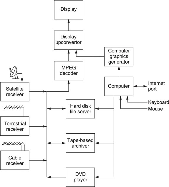
Note that when the hard drive is used to time shift or record, it simply stores the MPEG bitstream. On playback the bitstream is decoded and the picture quality will be unimpaired. The generation loss due to using an analog VCR is eliminated.

Ultimately digital technology will change the nature of television broadcasting out of recognition. Once the viewer has non-linear storage technology and electronic program guides, the traditional broadcaster’s transmitted schedule is irrelevant. Increasingly viewers will be able to choose what is watched and when, rather than the broadcaster deciding for them. The broadcasting of conventional commercials will cease to be effective when viewers have the technology to skip them. Anyone with a web site which can stream video can become a broadcaster.

1.2 What is a video signal?

When a two-dimensional image changes with time the basic information is three-dimensional. An analog electrical waveform is two-dimensional in that it carries a voltage changing with respect to time. In order to convey three-dimensional picture information down a two-dimensional channel it is necessary to resort to scanning. Instead of attempting to convey the brightness of all parts of a picture at once, scanning conveys the brightness of a single point which moves with time.

The scanning process converts spatial resolution on the image into the temporal frequency domain. The higher the resolution of the image, the more lines are necessary to resolve the vertical detail. The line rate is increased along with the number of cycles of modulation which need to be carried in each line. If the frame rate remains constant, the bandwidth goes up as the square of the resolution.

In an analog system, the video waveform is conveyed by some infinite variation of a continuous parameter such as the voltage on a wire or the strength or frequency of flux on a tape. In a recorder, distance along the medium is a further, continuous, analog of time. It does not matter at what point a recording is examined along its length, a value will be found for the recorded signal. That value can itself change with infinite resolution within the physical limits of the system.

Those characteristics are the main weakness of analog signals. Within the allowable bandwidth, any waveform is valid. If the speed of the medium is not constant, one valid waveform is changed into another valid waveform; a timebase error cannot be detected in an analog system. In addition, a voltage error simply changes one valid voltage into another; noise cannot be detected in an analog system. Noise might be suspected, but how is one to know what proportion of the received signal is noise and what is the original? If the transfer function of a system is not linear, distortion results, but the distorted waveforms are still valid; an analog system cannot detect distortion. Again distortion might be suspected, but it is impossible to tell how much of the energy at a given frequency is due to the distortion and how much was actually present in the original signal.

It is a characteristic of analog systems that degradations cannot be separated from the original signal, so nothing can be done about them. At the end of a system a signal carries the sum of all degradations introduced at each stage through which it passed. This sets a limit to the number of stages through which a signal can be passed before it is useless. Alternatively, if many stages are envisaged, each piece of equipment must be far better than necessary so that the signal is still acceptable at the end. The equipment will naturally be more expensive.

Digital video is simply an alternative means of carrying a moving image. Although there are a number of ways in which this can be done, there is one system, known as pulse code modulation (PCM) which is in virtually universal use.1 Figure 1.2 shows how PCM works. Instead of being continuous, the time axis is represented in a discrete, or stepwise manner. The video waveform is not carried by continuous representation, but by measurement at regular intervals. This process is called sampling and the frequency with which samples are taken is called the sampling rate or sampling frequency F_s

Figure 1.2 When a signal is carried in numerical form, either parallel or serial, the mechanisms described in the text ensure that the only degradation is in the conversion process.

In analog video systems, the time axis is sampled into frames, and the vertical axis is sampled into lines. Digital video simply adds a third sampling process along the lines. Each sample still varies infinitely as the original waveform did. To complete the conversion to PCM, each sample is then represented to finite accuracy by a discrete number in a process known as quantizing.

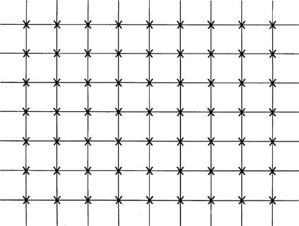
It is common to make the sampling rate a whole multiple of the line rate. Samples are then taken in the same place on every line. If this is done, a monochrome digital image becomes a rectangular array of points at which the brightness is stored as a number. The points are known as picture cells, pixels or pels. As shown in Figure 1.3, the array will generally be arranged with an even spacing between pixels, which are in rows and columns. Obviously the finer the pixel spacing, the greater the resolution of the picture will be, but the amount of data needed to store one picture will increase as the square of the resolution, and with it the costs.

Figure 1.3 A picture can be stored digitally by representing the brightness at each of the above points by a binary number. For a colour picture each point becomes a vector and has to describe the brightness, hue and saturation of that part of the picture. Samples are usually but not always formed into regular arrays of rows and columns, and it is most efficient if the horizontal and vertical spacing are the same.

At the ADC (analog-to-digital convertor), every effort is made to rid the sampling clock of jitter, or time instability, so every sample is taken at an exactly even time step. Clearly, if there is any subsequent timebase error, the instants at which samples arrive will be changed and the effect can be detected. If samples arrive at some destination with an irregular timebase, the effect can be eliminated by storing the samples temporarily in a memory and reading them out using a stable, locally generated clock. This process is called timebase correction and all properly engineered digital video systems must use it.

Those who are not familiar with digital principles often worry that sampling takes away something from a signal because it is not taking notice of what happened between the samples. This would be true in a system having infinite bandwidth, but no analog signal can have infinite bandwidth. All analog signal sources from cameras and so on have a resolution or frequency response limit, as indeed do devices such as CRTs and human vision. When a signal has finite bandwidth, the rate at which it can change is limited, and the way in which it changes becomes predictable. When a waveform can only change between samples in one way, it is then only necessary to convey the samples and the original waveform can be unambiguously reconstructed from them. A more detailed treatment of the principle will be given in Chapter 3.

As stated, each sample is also discrete, or represented in a stepwise manner. The magnitude of the sample, which will be proportional to the voltage of the video signal, is represented by a whole number. This process is known as quantizing and results in an approximation, but the size of the error can be controlled until it is negligible. The link between video quality and sample resolution is explored in Chapter 3. The advantage of using whole numbers is that they are not prone to drift.

If a whole number can be carried from one place to another without numerical error, it has not changed at all. By describing video waveforms numerically, the original information has been expressed in a way which is more robust.

Essentially, digital video carries the images numerically. Each sample is (in the case of luminance) an analog of the brightness at the appropriate point in the image.

1.3 Why binary?

Arithmetically, the binary system is the simplest numbering scheme possible. Figure 1.4(a) shows that there are only two symbols: 1 and 0. Each symbol is a binary digit, abbreviated to bit. One bit is a datum and many bits are data. Logically, binary allows a system of thought in which statements can only be true or false.

Figure 1.4 Binary digits (a) can only have two values. At (b) are shown some everyday binary terms, whereas (c) shows some terms which cannot be expressed by a binary digit.

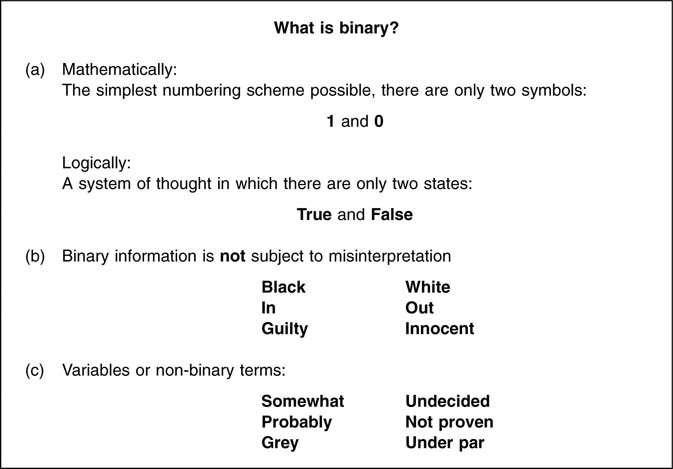
The great advantage of binary systems is that they are the most resistant to misinterpretation. In information terms they are robust. Figure 1.4(b) shows some binary terms and (c) some non-binary terms for comparison. In all real processes, the wanted information is disturbed by noise and distortion, but with only two possibilities to distinguish, binary systems have the greatest resistance to such effects.

Figure 1.5(a) shows an ideal binary electrical signal is simply two different voltages: a high voltage representing a true logic state or a binary 1 and a low voltage representing a false logic state or a binary 0. The ideal waveform is also shown at (b) after it has passed through a real system. The waveform has been considerably altered, but the binary information can be recovered by comparing the voltage with a threshold which is set half-way between the ideal levels. In this way any received voltage which is above the threshold is considered a 1 and any voltage below is considered a 0. This process is called slicing, and can reject significant amounts of unwanted noise added to the signal. The signal will be carried in a channel with finite bandwidth, and this limits the slew rate of the signal; an ideally upright edge is made to slope.

Figure 1.5 An ideal binary signal (a) has two levels. After transmission it may look like (b), but after slicing the two levels can be recovered. Noise on a sliced signal can result in jitter (c), but reclocking combined with slicing makes the final signal identical to the original as shown in (d).

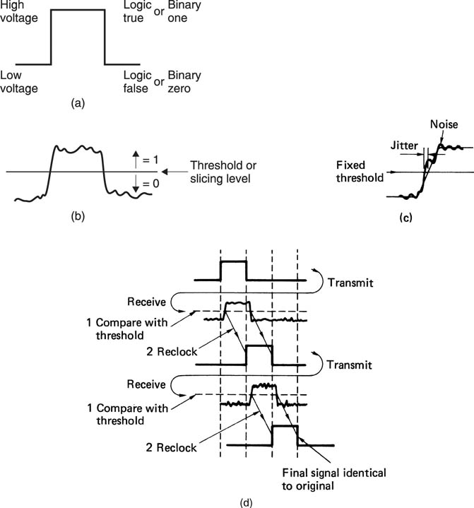
Noise added to a sloping signal (c) can change the time at which the slicer judges that the level passed through the threshold. This effect is also eliminated when the output of the slicer is reclocked. Figure 1.5(d) shows that however many stages the binary signal passes through, the information is unchanged except for a delay.

Of course, an excessive noise could cause a problem. If it had sufficient level and the correct sense or polarity, noise could cause the signal to cross the threshold and the output of the slicer would then be incorrect. However, as binary has only two symbols, if it is known that the symbol is incorrect, it need only be set to the other state and a perfect correction has been achieved. Error correction really is as trivial as that, although determining which bit needs to be changed is somewhat harder.

Figure 1.6 shows that binary information can be represented by a wide range of real phenomena. All that is needed is the ability to exist in two states. A switch can be open or closed and so represent a single bit. This switch may control the voltage in a wire which allows the bit to be transmitted. In an optical system, light may be transmitted or obstructed. In a mechanical system, the presence or absence of some feature can denote the state of a bit. The presence or absence of a radio carrier can signal a bit. In a random access memory (RAM), the state of an electric charge stores a bit.

Figure 1.6 A large number of real phenomena can be used to represent binary data.

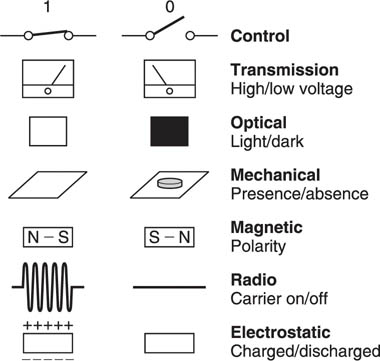
Figure 1.6 also shows that magnetism is naturally binary as two stable directions of magnetization are easily arranged and rearranged as required. This is why digital magnetic recording has been so successful: it is a natural way of storing binary signals.

The robustness of binary signals means that bits can be packed more densely onto storage media, increasing the performance or reducing the cost. In radio signalling, lower power can be used.

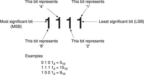
In decimal systems, the digits in a number (counting from the right, or least significant end) represent ones, tens, hundreds and thousands, etc. Figure 1.7 shows that in binary, the bits represent one, two, four, eight, sixteen, etc. A multidigit binary number is commonly called a word, and the number of bits in the word is called the wordlength. The right-hand bit is called the least significant bit (LSB) whereas the bit on the left-hand end of the word is called the most significant bit (MSB). Clearly more digits are required in binary than in decimal, but they are more easily handled. A word of eight bits is called a byte, which is a contraction of ‘by eight’.

Figure 1.7 also shows some binary numbers and their equivalent in decimal. The radix point has the same significance in binary: symbols to the right of it represent one half, one quarter and so on.

Figure 1.7 In a binary number, the digits represent increasing powers of two from the LSB. Also defined here are MSB and wordlength. When the wordlength is eight bits, the word is a byte. Binary numbers are used as memory addresses, and the range is defined by the address wordlength. Some examples are shown here.

Binary words can have a remarkable range of meanings. They may describe the magnitude of a number such as an audio sample or an image pixel or they may specify the address of a single location in a memory. In all cases the possible range of a word is limited by the wordlength. The range is found by raising two to the power of the wordlength. Thus a four-bit word has sixteen combinations, and could address a memory having sixteen locations. A sixteen-bit word has 65 536 combinations. Figure 1.8(a) shows some examples of wordlength and resolution.

Figure 1.8 The wordlength of a sample controls the resolution as shown in (a). In the same way the ability to address memory locations is also determined as in (b).

The capacity of memories and storage media is measured in bytes, but to avoid large numbers, kilobytes, megabytes and gigabytes are often used. A ten-bit word has 1024 combinations, which is close to one thousand. In digital terminology, 1 K is defined as 1024, so a kilobyte of memory contains 1024 bytes. A megabyte (1 MB) contains 1024 kilobytes and would need a twenty-bit address. A gigabyte contains 1024 megabytes and would need a thirty-bit address. Figure 1.8(b) shows some examples.

1.4 Colour

Colorimetry will be treated in Chapter 2 and it is intended to introduce only the basics here. Colour is created in television by the additive mixing in the display of three primary colours, red, green and blue. Effectively the display needs to be supplied with three video signals, each representing a primary colour. Since practical colour cameras generally also have three separate sensors, one for each primary colour, a camera and a display can be directly connected. RGB consists of three parallel signals each having the same spectrum, and is used where the highest accuracy is needed. RGB is seldom used for broadcast applications because of the high cost.

If RGB is used in the digital domain, it will be seen from Figure 1.9 that each image consists of three superimposed layers of samples, one for each primary colour. The pixel is no longer a single number representing a scalar brightness value, but a vector which describes in some way the brightness, hue and saturation of that point in the picture. In RGB, the pixels contain three unipolar numbers representing the proportion of each of the three primary colours at that point in the picture.

Some saving of bit rate can be obtained by using colour difference working. The human eye relies on brightness to convey detail, and much less resolution is needed in the colour information. Accordingly R, G and B are matrixed together to form a luminance (and monochrome-compatible) signal Y which needs full bandwidth. The eye is not equally sensitive to the three primary colours, as can be seen in Figure 1.10 and so the luminance signal is a weighted sum.

Figure 1.9 In the case of component video, each pixel site is described by three values and so the pixel becomes a vector quantity.

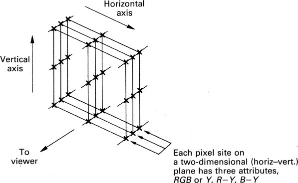
Figure 1.10 The response of the human eye to colour is not uniform.

The matrix also produces two colour difference signals, R–Y and B–Y. Colour difference signals do not need the same bandwidth as Y, because the eye’s acuity does not extend to colour vision. One half or one quarter of the bandwidth will do depending on the application.

In the digital domain, each pixel again contains three numbers, but one of these is a unipolar number representing the luminance and the other two are bipolar numbers representing the colour difference values. As the colour difference signals need less bandwidth, in the digital domain this translates to the use of a lower data rate, typically between one half and one sixteenth the bit rate of the luminance.

1.5 Why digital?

There are two main answers to this question, and it is not possible to say which is the most important, as it will depend on one’s standpoint.

Someone who is only interested in picture quality will judge the former the most relevant. If good-quality convertors can be obtained, all the shortcomings of analog recording and transmission can be eliminated to great advantage. One’s greatest effort is expended in the design of convertors, whereas those parts of the system which handle data need only be workmanlike. When a digital recording is copied, the same numbers appear on the copy: it is not a dub, it is a clone. If the copy is undistinguishable from the original, there has been no generation loss. Digital recordings can be copied indefinitely without loss of quality. This is, of course, wonderful for the production process, but when the technology becomes available to the consumer the issue of copyright becomes of great importance.

In the real world everything has a cost, and one of the greatest strengths of digital technology is low cost. When the information to be recorded is discrete numbers, they can be packed densely on the medium without quality loss. Should some bits be in error because of noise or dropout, error correction can restore the original value. Digital recordings take up less space than analog recordings for the same or better quality. Digital circuitry costs less to manufacture because more functionality can be put in the same chip.

Digital equipment can have self-diagnosis programs built-in. The machine points out its own failures so the the cost of maintenance falls. A small operation may not need maintenance staff at all; a service contract is sufficient. A larger organization will still need maintenance staff, but they will be fewer in number and their skills will be oriented more to systems than devices.

1.6 Some digital video processes outlined

Whilst digital video is a large subject, it is not necessarily a difficult one. Every process can be broken down into smaller steps, each of which is relatively easy to follow. The main difficulty with study is to appreciate where the small steps fit into the overall picture. Subsequent chapters of this book will describe the key processes found in digital technology in some detail, whereas this chapter illustrates why these processes are necessary and shows how they are combined in various ways in real equipment. Once the general structure of digital devices is appreciated, the following chapters can be put in perspective.

Figure 1.11(a) shows a minimal digital video system. This is no more than a point-to-point link which conveys analog video from one place to another. It consists of a pair of convertors and hardware to serialize and de-serialize the samples. There is a need for standardization in serial transmission so that various devices can be connected together. These standards for digital interfaces are described in Chapter 9.

Figure 1.11 In (a) two convertors are joined by a serial link. Although simple, this system is deficient because it has no means to prevent noise on the clock lines causing jitter at the receiver. In (b) a phase-locked loop is incorporated, which filters jitter from the clock.

Analog video entering the system is converted in the analog-to-digital convertor (ADC) to samples which are expressed as binary numbers. A typical sample would have a wordlength of eight bits. The sample is connected in parallel into an output register which controls the cable drivers. The cable also carries the sampling rate clock. The data are sent to the other end of the line where a slicer reflects noise picked up on each signal. Sliced data are then loaded into a receiving register by the clock, and sent to the digital-to-analog convertor (DAC), which converts the sample back to an analog voltage.

As Figure 1.5 showed, noise can change the timing of a sliced signal. Whilst this system rejects noise which threatens to change the numerical value of the samples, it is powerless to prevent noise from causing jitter in the receipt of the sample clock. Noise on the clock means that samples are not converted with a regular timebase and the impairment caused can be noticeable.

The jitter problem is overcome in Figure 1.11(b) by the inclusion of a phase-locked loop which is an oscillator that synchronizes itself to the average frequency of the clock but which filters out the instantaneous jitter.

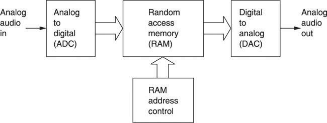
The system of Figure 1.11 is extended in Figure 1.12 by the addition of some random access memory (RAM). The operation of RAM is described in Chapter 2. What the device does is determined by the way in which the RAM address is controlled. If the RAM address increases by one every time a sample from the ADC is stored in the RAM, a recording can be made for a short period until the RAM is full. The recording can be played back by repeating the address sequence at the same clock rate but reading the memory into the DAC. The result is generally called a framestore.2 If the memory capacity is increased, the device can be used for recording. At a rate of 200 million bits per second, each frame needs a megabyte of memory and so the RAM recorder will be restricted to a fairly short playing time.

Figure 1.12 In the framestore, the recording medium is a random access memory (RAM). Recording time available is short compared with other media, but access to the recording is immediate and flexible as it is controlled by addressing the RAM.

Using compression, the playing time of a RAM-based recorder can be extended. For predetermined images such as test patterns and station IDs, read only memory (ROM) can be used instead as it is non-volatile.

1.7 Time compression and expansion

Data files such as computer programs are simply lists of instructions and have no natural time axis. In contrast, audio and video data are sampled at a fixed rate and need to be presented to the viewer at the same rate. In audiovisual systems the audio also needs to be synchronized to the video. Continuous bitstreams at a fixed bit rate are difficult for generic data recording and transmission systems to handle. Most digital recording and transmission systems work on blocks of data which can be individually addressed and/or routed. The bit rate may be fixed at the design stage at a value which may be too low or too high for the audio or video data to be handled.

The solution is to use time compression or expansion. Figure 1.13 shows a RAM which is addressed by binary counters which periodically overflow to zero and start counting again, giving the RAM a ring structure. If write and read addresses increment at the same speed, the RAM becomes a fixed data delay as the addresses retain a fixed relationship. However, if the read address clock runs at a higher frequency but in bursts, the output data are assembled into blocks with spaces in between. The data are now time compressed. Instead of being an unbroken stream which is difficult to handle, the data are in blocks with convenient pauses in between them. In these pauses numerous processes can take place. A hard disk might move its heads to another track. In all types of recording and transmission, the time compression of the samples allows time for synchronizing patterns, subcode and error-correction words to be inserted.

Figure 1.13 If the memory address is arranged to come from a counter which overflows, the memory can be made to appear circular. The write address then rotates endlessly, overwriting previous data once per revolution. The read address can follow the write address by a variable distance (not exceeding one revolution) and so a variable delay takes place between reading and writing.

Subsequently, any time compression can be reversed by time expansion. This requires a second RAM identical to the one shown. Data are written into the RAM in bursts, but read out at the standard sampling rate to restore a continuous bitstream. In a recorder, the time-expansion stage can be combined with the timebase correction stage so that speed variations in the medium can be eliminated at the same time. The use of time compression is universal in digital recording and widely used in transmission. In general the instantaneous data rate in the channel is not the same as the original rate although clearly the average rate must be the same.

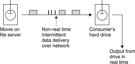
Where the bit rate of the communication path is inadequate, transmission is still possible, but not in real time. Figure 1.14 shows that the data to be transmitted will have to be written in real time on a storage device such as a disk drive, and the drive will then transfer the data at whatever rate is possible to another drive at the receiver. When the transmission is complete, the second drive can then provide the data at the corrrect bit rate.

Figure 1.14 In non-real-time transmission, the data are transferred slowly to a storage medium which then outputs real-time data. Movies can be downloaded to the home in this way.

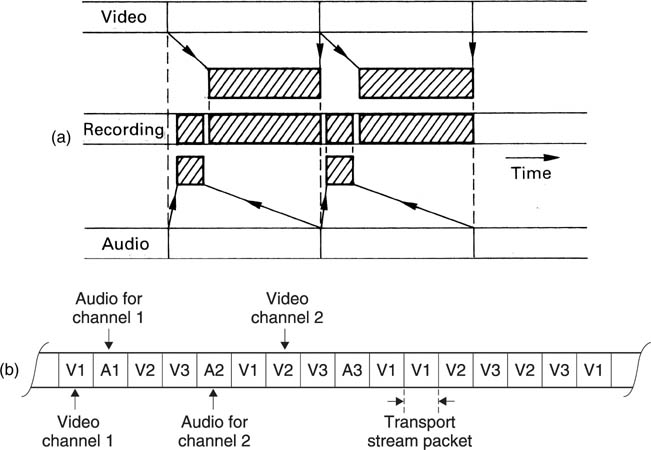
In the case where the available bit rate is higher than the correct data rate, the same configuration can be used to copy an audio or video data file faster than real time. Another application of time compression is to allow several streams of data to be carried along the same channel in a technique known as multiplexing. Figure 1.15 shows some examples. At (a) multiplexing allows audio and video data to be recorded on the same heads in a digital video recorder such as DVC. At (b), several TV channels are multiplexed into one MPEG transport stream.

Figure 1.15 (a) Time compression is used to shorten the length of track needed by the video. Heavily time-compressed audio samples can then be recorded on the same track using common circuitry. In MPEG, multiplexing allows data from several TV channels to share one bitstream (b).

1.8 Error correction and concealment

All practical recording and transmission media are imperfect. Magnetic media, for example, suffer from noise and dropouts. In a digital recording of binary data, a bit is either correct or wrong, with no intermediate stage. Small amounts of noise are rejected, but inevitably, infrequent noise impulses cause some individual bits to be in error. Dropouts cause a larger number of bits in one place to be in error. An error of this kind is called a burst error. Whatever the medium and whatever the nature of the mechanism responsible, data are either recovered correctly or suffer some combination of bit errors and burst errors. In optical disks, random errors can be caused by imperfections in the moulding process, whereas burst errors are due to contamination or scratching of the disk surface.

The visibility of a bit error depends upon which bit of the sample is involved. If the LSB of one sample was in error in a detailed, contrasty picture, the effect would be totally masked and no-one could detect it. Conversely, if the MSB of one sample was in error in a flat field, no-one could fail to notice the resulting spot. Clearly a means is needed to render errors from the medium inaudible. This is the purpose of error correction.

In binary, a bit has only two states. If it is wrong, it is only necessary to reverse the state and it must be right. Thus the correction process is trivial and perfect. The main difficulty is in identifying the bits which are in error. This is done by coding the data by adding redundant bits. Adding redundancy is not confined to digital technology, airliners have several engines and cars have twin braking systems. Clearly the more failures which have to be handled, the more redundancy is needed. If a four-engined airliner is designed to fly normally with one engine failed, three of the engines have enough power to reach cruise speed, and the fourth is redundant. The amount of redundancy is equal to the amount of failure which can be handled. In the case of the failure of two engines, the plane can still fly, but it must slow down; this is graceful degradation. Clearly the chances of a two-engine failure on the same flight are remote.

In digital recording, the amount of error which can be corrected is proportional to the amount of redundancy, and it will be shown in Chapter 6 that within this limit, the samples are returned to exactly their original value. Consequently corrected samples are undetectable. If the amount of error exceeds the amount of redundancy, correction is not possible, and, in order to allow graceful degradation, concealment will be used. Concealment is a process where the value of a missing sample is estimated from those nearby. The estimated sample value is not necessarily exactly the same as the original, and so under some circumstances concealment can be audible, especially if it is frequent. However, in a well-designed system, concealments occur with negligible frequency unless there is an actual fault or problem.

Concealment is made possible by rearranging the sample sequence prior to recording. This is shown in Figure 1.16 where odd-numbered samples are separated from even-numbered samples prior to recording. The odd and even sets of samples may be recorded in different places on the medium, so that an uncorrectable burst error affects only one set. On replay, the samples are recombined into their natural sequence, and the error is now split up so that it results in every other sample being lost in a two-dimensional structure. The picture is now described half as often, but can still be reproduced with some loss of accuracy. This is better than not being reproduced at all even if it is not perfect. Many digital video recorders use such an odd/even distribution for concealment. Clearly if any errors are fully correctable, the distribution is a waste of time; it is only needed if correction is not possible.

Figure 1.16 In cases where the error correction is inadequate, concealment can be used provided that the samples have been ordered appropriately in the recording. Odd and even samples are recorded in different places as shown here. As a result an uncorrectable error causes incorrect samples to occur singly, between correct samples. In the example shown, sample 8 is incorrect, but samples 7 and 9 are unaffected and an approximation to the value of sample 8 can be had by taking the average value of the two. This interpolated value is substituted for the incorrect value.

The presence of an error-correction system means that the video (and audio) quality is independent of the medium/head quality within limits. There is no point in trying to assess the health of a machine by watching a monitor or listening to the audio, as this will not reveal whether the error rate is normal or within a whisker of failure. The only useful procedure is to monitor the frequency with which errors are being corrected, and to compare it with normal figures.

1.9 Product codes

Digital systems such as broadcasting, optical disks and magnetic recorders are prone to burst errors. Adding redundancy equal to the size of expected bursts to every code is inefficient. Figure 1.17(a) shows that the efficiency of the system can be raised using interleaving. Sequential samples from the ADC are assembled into codes, but these are not recorded/transmitted in their natural sequence. A number of sequential codes are assembled along rows in a memory. When the memory is full, it is copied to the medium by reading down columns. Subsequently, the samples need to be de-interleaved to return them to their natural sequence. This is done by writing samples from tape into a memory in columns, and when it is full, the memory is read in rows. Samples read from the memory are now in their original sequence so there is no effect on the information. However, if a burst error occurs as is shown shaded on the diagram, it will damage sequential samples in a vertical direction in the de-interleave memory. When the memory is read, a single large error is broken down into a number of small errors whose size is exactly equal to the correcting power of the codes and the correction is performed with maximum efficiency.

Figure 1.17a Interleaving is essential to make error-correction schemes more efficient. Samples written sequentially in rows into a memory have redundancy P added to each row. The memory is then read in columns and the data sent to the recording medium. On replay the non-sequential samples from the medium are de-interleaved to return them to their normal sequence. This breaks up the burst error (shaded) into one error symbol per row in the memory, which can be corrected by the redundancy P.

An extension of the process of interleave is where the memory array has not only rows made into codewords but also columns made into codewords by the addition of vertical redundancy. This is known as a product code. Figure 1.17(b) shows that in a product code the redundancy calculated first and checked last is called the outer code, and the redundancy calculated second and checked first is called the inner code. The inner code is formed along tracks on the medium. Random errors due to noise are corrected by the inner code and do not impair the burst-correcting power of the outer code. Burst errors are declared uncorrectable by the inner code which flags the bad samples on the way into the de-interleave memory. The outer code reads the error flags in order to locate the erroneous data. As it does not have to compute the error locations, the outer code can correct more errors.

Figure 1.17b In addition to the redundancy P on rows, inner redundancy Q is also generated on columns. On replay, the Q code checker will pass on flag F if it finds an error too large to handle itself. The flags pass through the de-interleave process and are used by the outer error correction to identify which symbol in the row needs correcting with P redundancy. The concept of crossing two codes in this way is called a product code.

The interleave, de-interleave, time-compression and timebase-correction processes inevitably cause delay.

1.10 Shuffling

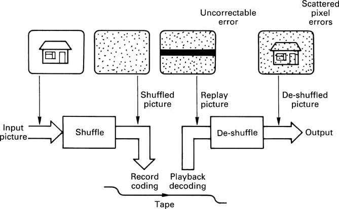
When a product code-based recording suffers an uncorrectable error the result is a rectangular block of failed sample values which require concealment. Such a regular structure would be visible even after concealment, and an additional process is necessary to reduce the visibility. Figure 1.18 shows that a shuffle process is performed prior to product coding in which the pixels are moved around the picture in a pseudo-random fashion. The reverse process is used on replay, and the overall effect is nullified. However, if an uncorrectable error occurs, this will only pass through the de-shuffle and so the regular structure of the failed data blocks will be randomized. The errors are spread across the picture as individual failed pixels in an irregular structure. Chapter 11 treats shuffling techniques in more detail.

Figure 1.18 The shuffle before recording and the corresponding de-shuffle after playback cancel out as far as the picture is concerned. However, a block of errors due to dropout only experiences the de-shuffle, which spreads the error randomly over the screen. The pixel errors are then easier to correct.

1.11 Channel coding

In most recorders used for storing digital information, the medium carries a track which reproduces a single waveform. Clearly data words representing video contain many bits and so they have to be recorded serially, a bit at a time. Some media, such as optical or magnetic disks, have only one active track, so it must be totally self-contained. DVTRs may have one, two or four tracks read or written simultaneously. At high recording densities, physical tolerances cause phase shifts, or timing errors, between tracks and so it is not possible to read them in parallel. Each track must still be self-contained until the replayed signal has been timebase corrected.

Recording data serially is not as simple as connecting the serial output of a shift register to the head. In digital video, samples may contain strings of identical bits. If a shift register is loaded with such a sample and shifted out serially, the output stays at a constant level for the period of the identical bits, and nothing is recorded on the track. On replay there is nothing to indicate how many bits were present, or even how fast to move the medium. Clearly, serialized raw data cannot be recorded directly, it has to be modulated into a waveform which contains an embedded clock irrespective of the values of the bits in the samples. On replay a circuit called a data separator can lock to the embedded clock and use it to separate strings of identical bits.

The process of modulating serial data to make it self-clocking is called channel coding. Channel coding also shapes the spectrum of the serialized waveform to make it more efficient. With a good channel code, more data can be stored on a given medium. Spectrum shaping is used in optical disks to prevent the data from interfering with the focus and tracking servos, and in hard disks and in certain DVTRs to allow rerecording without erase heads.

Channel coding is also needed to broadcast digital television signals where shaping of the spectrum is an obvious requirement to avoid interference with other services.

The techniques of channel coding for recording are covered in detail in Chapter 6, whereas the modulation schemes for digital television are described in Chapter 9.

1.12 Video compression and MPEG

In its native form, digital video suffers from an extremely high data rate, particularly in high definition. One approach to the problem is to use compression which reduces that rate significantly with a moderate loss of subjective quality of the picture. The human eye is not equally sensitive to all spatial frequencies, so some coding gain can be obtained by using fewer bits to describe the frequencies which are less visible. Video images typically contain a great deal of redundancy where flat areas contain the same pixel value repeated many times. Furthermore, in many cases there is little difference between one picture and the next, and compression can be achieved by sending only the differences.

Whilst these techniques may achieve considerable reduction in bit rate, it must be appreciated that compression systems reintroduce the generation loss of the analog domain to digital systems. As a result high compression factors are only suitable for final delivery of fully produced material to the viewer.

For production purposes, compression may be restricted to exploiting the redundancy within each picture individually and then with a mild compression factor. This allows simple algorithms to be used and also permits multiple-generation work without artifacts being visible. A similar approach is used in disk-based workstations. Where off-line editing is used (see Chapter 13) higher compression factors can be employed as the impaired pictures are not seen by the viewer.

Clearly, a consumer DVTR needs only single-generation operation and has simple editing requirements. A much greater degree of compression can then be used, which may take advantage of redundancy between fields. The same is true for broadcasting, where bandwidth is at a premium. A similar approach may be used in disk-based camcorders which are intended for ENG purposes.

The future of television broadcasting (and of any high-definition television) lies completely in compression technology. Compression requires an encoder prior to the medium and a compatible decoder after it. Extensive consumer use of compression could not occur without suitable standards. The ISO-MPEG coding standards were specifically designed to allow wide interchange of compressed video data. Digital television broadcasting and the digital video disk both use MPEG standard bitstreams.

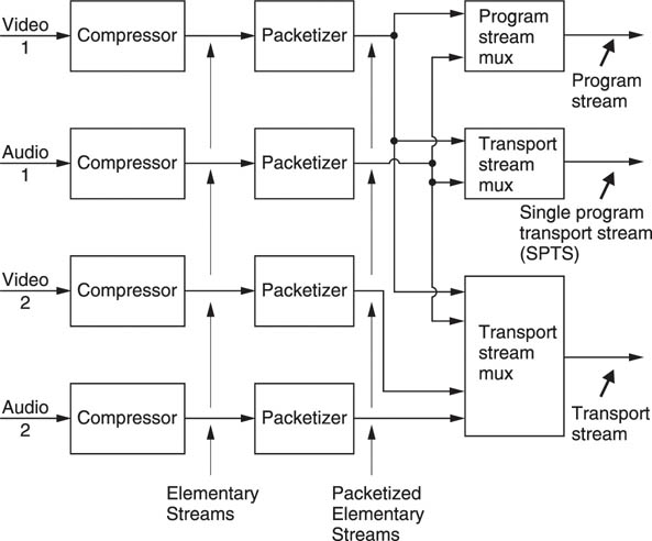
Figure 1.19 shows that the output of a single compressor is called an elementary stream. In practice audio and video streams of this type can be combined using multiplexing. The program stream is optimized for recording and is based on blocks of arbitrary size. The transport stream is optimized for transmission and is based on blocks of constant size.

Figure 1.19 The bitstream types of MPEG-2. See text for details.

In production equipment such as workstations and VTRs which are designed for editing, the MPEG standard is less useful and many successful products use non-MPEG compression.

Compression and the corresponding decoding are complex processes and take time, adding to existing delays in signal paths. Concealment of uncorrectable errors is also more difficult on compressed data.

1.13 Disk-based recording

The magnetic disk drive was perfected by the computer industry to allow rapid random access to data, and so it makes an ideal medium for editing. As will be seen in Chapter 7, the heads do not touch the disk, but are supported on a thin air film which gives them a long life but which restricts the recording density. Thus disks cannot compete with tape for lengthy recordings, but for short-duration work such as commercials or animation they have no equal. The data rate of digital video is too high for a single disk head, and so a number of solutions have been explored. One obvious solution is to use compression, which cuts the data rate and extends the playing time. Another approach is to operate a large array of conventional drives in parallel. The highest-capacity magnetic disks are not removable from the drive.

The disk drive provides intermittent data transfer owing to the need to reposition the heads. Figure 1.20 shows that disk-based devices rely on a quantity of RAM acting as a buffer between the real-time video environment and the intermittent data environment.

Figure 1.20 In a hard disk recorder, a large-capacity memory is used as a buffer or timebase corrector between the convertors and the disk. The memory allows the convertors to run constantly despite the interruptions in disk transfer caused by the head moving between tracks.

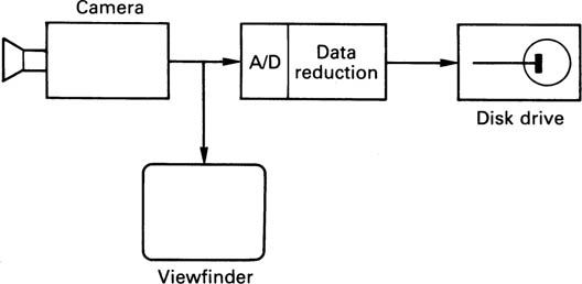
Figure 1.21 shows the block diagram of a camcorder based on hard disks and compression. The recording time and picture quality will not compete with full bandwidth tape-based devices, but following acquisition the disks can be used directly in an edit system, allowing a useful time saving in ENG applications.

Figure 1.21 In a disk-based camcorder, the PCM data rate from the camera is too high for direct recording on disk. Data reduction is used to cut the bit rate and extend playing time. If a standard file structure is used, disks may physically be transferred to an edit system after recording.

Development of the optical disk was stimulated by the availability of low-cost lasers. Optical disks are available in many different types, some which can only be recorded once, some which are erasable. These will be contrasted in Chapter 7. Optical disks have in common the fact that access is generally slower than with magnetic drives and it is difficult to obtain high data rates, but most of them are removable and can act as interchange media.

1.14 Rotary-head digital recorders

The rotary-head recorder has the advantage that the spinning heads create a high head-to-tape speed offering a high bit rate recording without high tape speed. Whilst mechanically complex, the rotary-head transport has been raised to a high degree of refinement and offers the highest recording density and thus lowest cost per bit of all digital recorders.3

Digital VTRs segment incoming fields into several tape tracks and invisibly reassemble them in memory on replay in order to keep the tracks reasonably short.

Figure 1.22 shows a representative block diagram of a DVTR. Following the convertors, a compression process may be found. In an uncompressed recorder, there will be distribution of odd and even samples and a shuffle process for concealment purposes. An interleaved product code will be formed prior to the channel coding stage which produces the recorded waveform. On replay the data separator decodes the channel code and the inner and outer codes perform correction as in section 1.9. Following the de-shuffle the data channels are recombined and any necessary concealment will take place. Any compression will be decoded prior to the output convertors.

Figure 1.22 Block diagram of a DVTR. Note optional data reduction unit which may be used to allow a common transport to record a variety of formats.

1.15 DVD and DVHS

DVD (digital video disk) and DVHS (digital VHS) are formats intended for home use. DVD is a prerecorded optical disk which carries an MPEG program stream containing a moving picture and one or more audio channels. DVD in many respects is a higher density development of Compact Disc technology.

DVHS is a development of the VHS system which records MPEG data. In a digital television broadcast receiver, an MPEG transport stream is demodulated from the off-air signal. Transport streams contain several TV programs and the one required is selected by demultiplexing. As DVHS can record a transport stream, it can record more than one program simultaneously, with the choice being made on playback.

1.16 Digital television broadcasting

Although it has given good service for many years, analog television broadcasting is extremely inefficient because the transmitted waveform is directly compatible with the CRT display, and nothing is transmitted during the blanking periods whilst the beam retraces. Using compression, digital modulation and error-correction techniques, the same picture quality can be obtained in a fraction of the bandwidth of analog. Pressure on spectrum use from other uses such as cellular telephones will only increase and this will ensure rapid changeover to digital television and radio broadcasts.

If broadcasting of high-definition television is ever to become widespread it will do so via digital compressed transmission as the bandwidth required will otherwise be hopelessly uneconomic. In addition to conserving spectrum, digital transmission is (or should be) resistant to multipath reception and gives consistent picture quality throughout the service area.

1.17 Networks

Communications networks allow transmission of data files whose content or meaning is irrelevant to the transmission medium. These files can therefore contain digital video. Video production systems can be based on high bit rate networks instead of traditional video-routing techniques. Contribution feeds between broadcasters and station output to transmitters no longer requires special-purpose links. Video delivery is also possible on the Internet. As a practical matter, most Internet users suffer from a relatively limited bit rate and if moving pictures are to be sent, a very high compression factor will have to be used. Pictures with a relatively small number of lines and much reduced frame rates will be needed. Whilst the quality does not compare with that of broadcast television, this is not the point. Internet video allows a wide range of services which traditional broadcasting cannot provide and phenomenal growth is expected in this area.

References

1. Devereux, V.G., Pulse code modulation of video signals: 8 bit coder and decoder. BBC Res. Dept. Rept., EL-42, No.25 (1970)

2. Pursell, S. and Newby, H., Digital frame store for television video. SMPTE Journal, 82, 402–403 (1973)

3. Baldwin, J.L.E., Digital television recording – history and background. SMPTE Journal, 95, 1206–1214 (1986)