
Simulator Overview
Simulation enables you to discover the distribution of model outputs as a function of the random variation in the factors and model noise. The simulation facility in the profilers provides a way to set up the random inputs and run the simulations, producing an output table of simulated values.
An example of this facility’s use would be to find out the defect rate of a process that has been fit, and see whether it is robust with respect to variation in the factors. If specification limits have been set in the responses, they are carried over into the simulation output, allowing a prospective capability analysis of the simulated model using new factors settings.
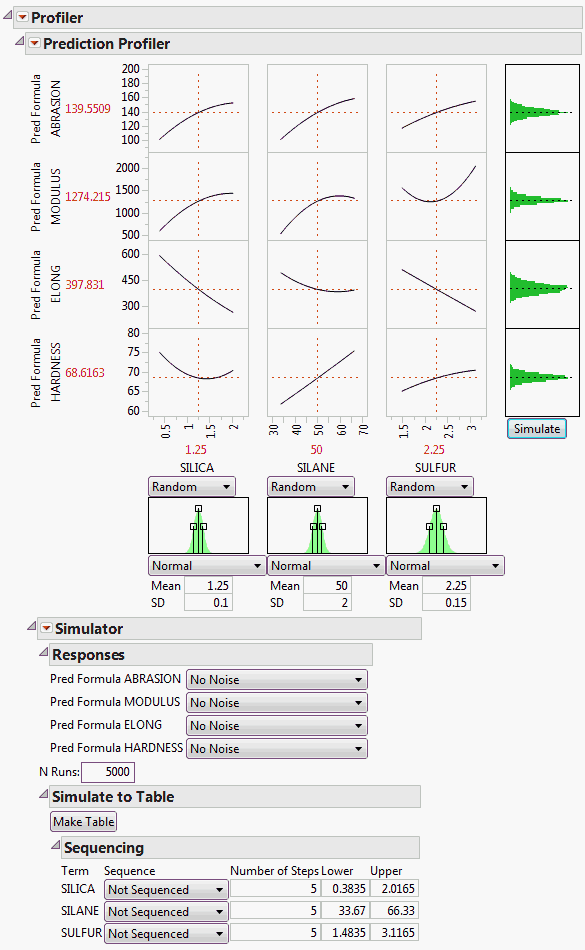
In the Profiler, the Simulator is integrated into the graphical layout. Factor specifications are aligned below each factor’s profile. A simulation histogram is shown on the right for each response.
Figure 8.2 Profiler with Simulator
In the other profilers, the Simulator is less graphical, and kept separate. There are no integrated histograms, and the interface is textual. However, the internals and output tables are the same.
Example of Running the Simulation
Tip: The Make Table and Sequencing options are most useful when you have random values. Sequencing options are available for the following distributions only: Normal, Uniform, and Triangular.
Specify the number of runs in the simulation by entering it in the N Runs box.
After the factor and response distributions are set, click the Simulate button to run the simulation. Or, use the Make Table button to create a table with N Runs for the number of rows. Each row is populated with a random draw from the specified distributions, and the corresponding response values are computed. If spec limits are given, the table also contains a column specifying whether a row is in or out of spec.
Use sequencing to examine how the distribution of the response changes when the mean (sequencing location) and variability (sequencing spread) of the inputs change.
Sequencing Example
1. Open the Tiretread.jmp sample data table.
2. Select Graph > Profiler.
3. Select Pred Formula ABRASION and Pred Formula MODULUS and click Y, Prediction Formula.
4. Click OK.
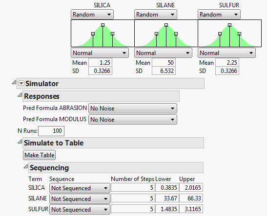
5. From the red triangle menu next to Prediction Profiler, select Simulator.
6. Change each factor to be Random instead of Fixed.
7. Change the N Runs value to 100.
8. Open Simulate to Table then Sequencing.
Figure 8.3 Simulator Settings
You want to examine how the responses change when the mean values change.
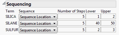
9. For SILICA, select Sequence Location. Keep the number of steps at 5. Because the mean is 1.25, change the values over a range of 1 (lower) to 2 (upper).
10. For SILANE, select Sequence Location. Keep the number of steps at 5. Because the mean is 50, change the values over a range of 40 (lower) to 50 (upper).
11. For SULFUR, select Sequence Location. Keep the number of steps at 5. Because the mean is 2.25, change the values over a range of 2 (lower) to 3 (upper).
Figure 8.4 Sequencing Settings
12. Click Make Table.
You can see that the SILICA Mean, SILANE Mean, and SULFUR Mean columns contain five steps for each range of values (Silica Mean is 1, 1.25, 1.5, 1.75, and 2; Silane Mean is 40, 42.5, 45, 47.5, and 50; and so on.) Pred Formula ABRASION and Pred Formula MODULUS values are calculated for each combination of values, so you can see how the responses change as the factor values change.
13. Select Analyze > Distribution.
14. Select Pred Formula ABRASION and SILICA Mean and click Y, Columns.
15. Click OK.
Figure 8.5 Distribution of SILICA Mean by Pred Formula ABRASION
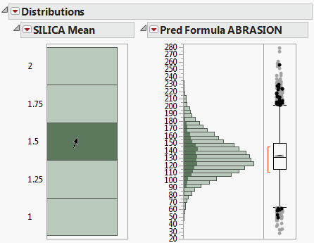
Click a histogram bar that corresponds to a SILICA mean to see how the prediction formula for ABRASION changes given the selected mean.
Specifying Factors
Factors (inputs) and responses (outputs) are already given roles by being in the Profiler. Additional specifications for the simulator are on how to give random values to the factors, and add random noise to the responses.
For each factor, the choices of how to give values are as follows:
Fixed
Fixes the factor at the specified value. The initial value is the current value in the profiler, which might be a value obtained through optimization.
Random
Gives the factor the specified distribution and distributional parameters.
See the Using JMP book for descriptions of most of these random functions. If the factor is categorical, then the distribution is characterized by probabilities specified for each category, with the values normalized to sum to 1.
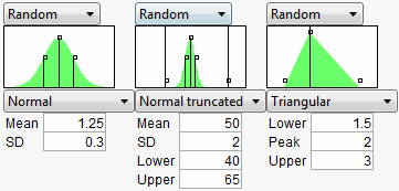
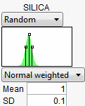
Normal weighted is normally distributed with the given mean and standard deviation, but a special stratified and weighted sampling system is used to simulate very rare events far out into the tails of the distribution. This is a good choice when you want to measure very low defect rates accurately. See “Statistical Details”.
Normal truncated is a normal distribution limited by lower and upper limits. Any random realization that exceeds these limits is discarded and the next variate within the limits is chosen. This is used to simulate an inspection system where inputs that do not satisfy specification limits are discarded or sent back.
Normal censored is a normal distribution limited by lower and upper limits. Any random realization that exceeds a limit is just set to that limit, putting a density mass on the limits. This is used to simulate a re-work system where inputs that do not satisfy specification limits are reworked until they are at that limit.
Sampled means that JMP selects values at random from that column in the data table.
External means that JMP selects values at random from a column in another table. You are prompted to choose the table and column.
The Aligned check box is used for two or more Sampled or External sources. When checked, the random draws come from the same row of the table. This is useful for maintaining the correlation structure between two columns. If the Aligned option is used to associate two columns in different tables, the columns must have equal number of rows.
In the Profiler, a graphical specification shows the form of the density for the continuous distributions, and provides control points that can be dragged to change the distribution. The drag points for the Normal are the mean and the mean plus or minus one standard deviation. The Normal truncated and censored add points for the lower and upper limits. The Uniform and Triangular have limit control points, and the Triangular adds the mode.
Figure 8.6 Distributions
Expression
Allows you to write your own expression in JMP Scripting Language (JSL) form into a field. This gives you flexibility to make up a new random distribution. For example, you could create a censored normal distribution that guaranteed nonnegative values with an expression like Max(0,RandomNormal(5,2)). In addition, character results are supported, so If(Random Uniform() < 0.2, “M”, “F”) works fine. After entering the expression, click the Reset button to submit the expression.
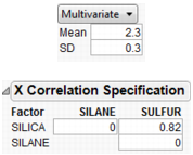
Multivariate
Allows you to generate a multivariate normal for when you have correlated factors. Specify the mean and standard deviation with the factor, and a correlation matrix separately.
Figure 8.7 Using a Correlation Matrix
Responses Report Options
If the model is only partly a function of the factors, and the rest of the variation of the response is attributed to random noise, then you will want to specify this with the responses. The choices are:
No Noise
Evaluates the response from the model, with no additional random noise added.
Add Random Noise
Obtains the response by adding a normal random number with the specified standard deviation to the evaluated model.
Add Random Weighted Noise
Is distributed like Add Random Noise, but with weighted sampling to enable good extreme tail estimates.
Add Multivariate Noise
Yields a response as follows: A multivariate random normal vector is obtained using a specified correlation structure, and it is scaled by the specified standard deviation and added to the value obtained by the model.
Simulator Report Options
Automatic Histogram Update
Toggles histogram update, which sends changes to all histograms shown in the Profiler, so that histograms update with new simulated values when you drag distribution handles.
Defect Profiler
Shows the defect rate as an isolated function of each factor. This command is enabled when spec limits are available, as described below.
Defect Parametric Profile
Shows the defect rate as an isolated function of the parameters of each factor’s distribution. It is enabled when the Defect Profiler is launched.
Simulation Experiment
Used to run a designed simulation experiment on the locations of the factor distributions. A window appears, allowing you to specify the number of design points, the portion of the factor space to be used in the experiment, and which factors to include in the experiment. For factors not included in the experiment, the current value shown in the Profiler is the one used in the experiment.
The experimental design is a Latin Hypercube. The output has one row for each design point. The responses include the defect rate for each response with spec limits, and an overall defect rate. After the experiment, it would be appropriate to fit a Gaussian Process model on the overall defect rate, or a root or a logarithm of it.
A simulation experiment does not sample the factor levels from the specified distributions. As noted above, the design is a Latin Hypercube. At each design point, N Runs random draws are generated with the design point serving as the center of the random draws, and the shape and variability coming from the specified distributions.
Spec Limits
Shows or edits specification limits.
N Strata
Is a hidden option accessible by holding down the Shift key before clicking the Simulator red triangle menu. This option enables you to specify the number of strata in Normal Weighted. For more information also see “Statistical Details”.
Set Random Seed
Is a hidden option accessible by holding down the Shift key before clicking the Simulator red triangle menu. This option enables you to specify a seed for the simulation starting point. This enables the simulation results to be reproducible, unless the seed is set to zero. The seed is set to zero by default. If the seed is nonzero, then the latest simulation results are output if the Make Table button is clicked.
Using Specification Limits
The profilers support specification limits on the responses, providing a number of features
• In the Profiler, if you do not have the Response Limits property set up in the input data table to provide desirability coordinates, JMP looks for a Spec Limits property and constructs desirability functions appropriate to those Spec Limits.
• If you use the Simulator to output simulation tables, JMP copies Spec Limits to the output data tables, making accounting for defect rates and capability indices easy.
• Adding Spec Limits enables a feature called the Defect Profiler.
In the following example, we assume that the following Spec Limits have been specified.
|
Response
|
LSL
|
USL
|
|
Abrasion
|
110
|
|
|
Modulus
|
|
2000
|
|
Elong
|
350
|
550
|
|
Hardness
|
66
|
74
|
To set these limits in the data table, highlight a column and select Cols > Column Info. Then, click the Column Properties button and select the Spec Limits property.
If you are already in the Simulator in a profiler, another way to enter them is to use the Spec Limits command in the Simulator red triangle menu.
Figure 8.8 Spec Limits
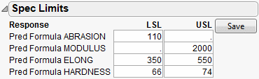
After entering the spec limits, they are incorporated into the profilers. Click the Save button if you want the spec limits saved back to the data table as a column property.
With these specification limits, and the distributions shown in Figure 8.2, click the Simulate button. Notice the spec limit lines in the output histograms.
Figure 8.9 Spec Limits in the Prediction Profiler
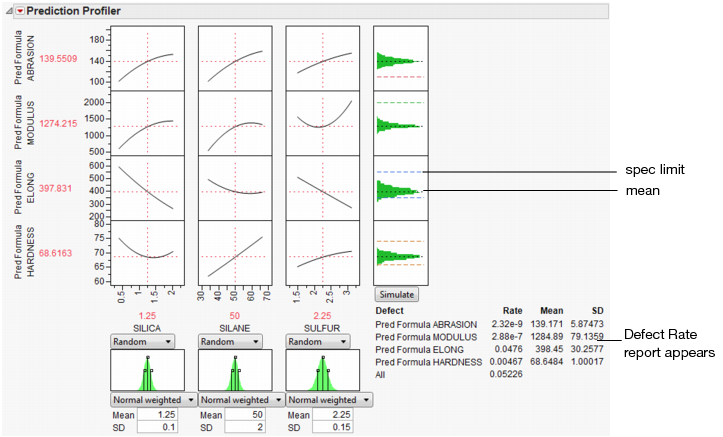
Look at the histogram for Abrasion. The lower spec limit is far above the distribution, yet the Simulator is able to estimate a defect rate for it. This despite only having 5000 runs in the simulation. It can do this rare-event estimation when you use a Normal weighted distribution.
Note that the Overall defect rate is close to the defect rate for ELONG, indicating that most of the defects are in the ELONG variable.
To see this weighted simulation in action, click the Make Table button and examine the Weight column.
JMP generates extreme values for the later observations, using very small weights to compensate. Because the Distribution platform handles frequencies better than weights, there is also a column of frequencies, which is simply the weights multiplied by 1012.
The output data set contains a Distribution script appropriate to analyze the simulation data completely with a capability analysis.
Simulating General Formulas
Though the profiler and simulator are designed to work from formulas stored from a model fit, they work for any formula that can be stored in a column. A typical application of simulation is to exercise financial models under certain probability scenarios to obtain the distribution of the objectives. This can be done in JMP—the key is to store the formulas into columns, set up ranges, and then conduct the simulation.
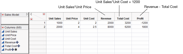
|
Inputs
(Factors)
|
Unit Sales
|
random uniform between 1000 and 2000
|
|
Unit Price
|
fixed
|
|
|
Unit Cost
|
random normal with mean 2.25 and std dev 0.1
|
|
|
Outputs
(Responses)
|
Revenue
|
formula: Unit Sales*Unit Price
|
|
Total Cost
|
formula: Unit Sales*Unit Cost + 1200
|
|
|
Profit
|
formula: Revenue – Total Cost
|
The following JSL script creates the data table below with some initial scaling data and stores formulas into the output variables. It also launches the Profiler.
dt = newTable("Sales Model");
dt<<newColumn("Unit Sales",Values({1000,2000}));
dt<<newColumn("Unit Price",Values({2,4}));
dt<<newColumn("Unit Cost",Values({2,2.5}));
dt<<newColumn("Revenue",Formula(:Unit Sales*:Unit Price));
dt<<newColumn("Total Cost",Formula(:Unit Sales*:Unit Cost + 1200));
dt<<newColumn("Profit",Formula(:Revenue-:Total Cost), Set Property(“Spec Limits”,{LSL(0)}));
Profiler(Y(:Revenue,:Total Cost,:Profit), Objective Formula(Profit));
Figure 8.10 Data Table Created from Script
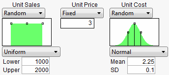
Once they are created, select the Simulator from the Prediction Profiler. Use the specifications from Table 8.2 to fill in the Simulator.
Figure 8.11 Profiler Using the Data Table
Now, run the simulation, which produces the following histograms in the Profiler.
Figure 8.12 Simulator
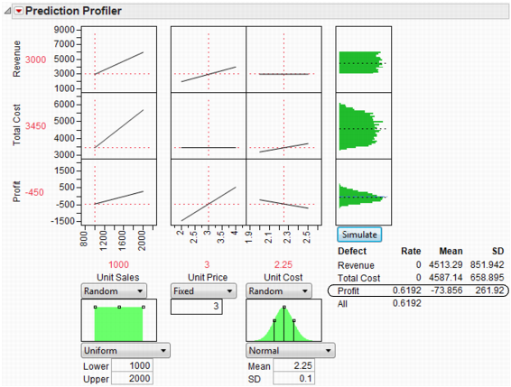
It looks like we are not very likely to be profitable. By putting a lower specification limit of zero on Profit, the defect report would say that the probability of being unprofitable is 62%.
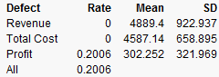
So we raise the Unit Price to $3.25 and rerun the simulation. Now the probability of being unprofitable is down to about 21%.
Figure 8.13 Results
If unit price cannot be raised anymore, you should now investigate lowering your cost, or increasing sales, if you want to further decrease the probability of being unprofitable.
The Defect Profiler
The defect profiler shows the probability of an out-of-spec output defect as a function of each factor, while the other factors vary randomly. This is used to help visualize which factor’s distributional changes the process is most sensitive to, in the quest to improve quality and decrease cost.
Specification limits define what is a defect, and random factors provide the variation to produce defects in the simulation. Both need to be present for a Defect Profile to be meaningful.
At least one of the Factors must be declared Random for a defect simulation to be meaningful, otherwise the simulation outputs would be constant. These are specified though the simulator Factor specifications.
Important: If you need to estimate very small defect rates, use Normal weighted instead of just Normal. This allows defect rates of just a few parts per million to be estimated well with only a few thousand simulation runs.
About Tolerance Design
Tolerance Design is the investigation of how defect rates on the outputs can be controlled by controlling variability in the input factors.
The input factors have variation. Specification limits are used to tell the supplier of the input what range of values are acceptable. These input factors then go into a process producing outputs, and the customer of the outputs then judges if these outputs are within an acceptable range.
Sometimes, a Tolerance Design study shows that spec limits on input are unnecessarily tight, and loosening these limits results in cheaper product without a meaningful sacrifice in quality. In these cases, Tolerance Design can save money.
In other cases, a Tolerance Design study might find that either tighter limits or different targets result in higher quality. In all cases, it is valuable to learn which inputs the defect rate in the outputs are most sensitive to.
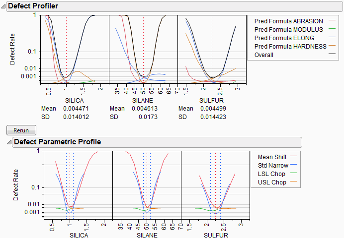
This graph shows the defect rate as a function of each factor as if it were a constant, but all the other factors varied according to their random specification. If there are multiple outputs with Spec Limits, then there is a defect rate curve color-coded for each output. A black curve shows the overall defect rate—this curve is above all the colored curves.
Figure 8.14 Defect Profiler
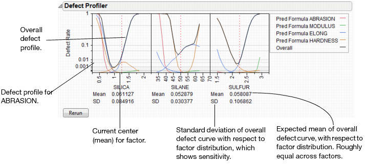
Graph Scale
Defect rates are shown on a cubic root scale, so that small defect rates are shown in some detail even though large defect rates might be visible. A log scale is not used because zero rates are not uncommon and need to be shown.
Expected Defects
Reported below each defect profile plot is the mean and standard deviation (SD). The mean is the overall defect rate, calculated by integrating the defect profile curve with the specified factor distribution.
In this case, the defect rate that is reported below all the factors is estimating the same quantity, the rate estimated for the overall simulation below the histograms (that is, if you clicked the Simulate button). Because each estimate of the rate is obtained in a different way, they might be a little different. If they are very different, you might need to use more simulation runs. In addition, check that the range of the factor scale is wide enough so that the integration covers the distribution well.
The standard deviation is a good measure of the sensitivity of the defect rates to the factor. It is quite small if either the factor profile were flat, or the factor distribution has a very small variance. Comparing SD's across factors is a good way to know which factor should get more attention to reducing variation.
The mean and SD are updated when you change the factor distribution. This is one way to explore how to reduce defects as a function of one particular factor at a time. You can click and drag a handle point on the factor distribution, and watch the mean and SD change as you drag. However, changes are not updated across all factors until you click the Rerun button to do another set of simulation runs.
Simulation Method and Details
Assume we want a defect profile for factor X1, in the presence of random variation in X2 and X3. A series of n=N Runs simulation runs is done at each of k points in a grid of equally spaced values of X1. (k is generally set at 17). At each grid point, suppose that there are m defects due to the specification limits. At that grid point, the defect rate is m/n. With normal weighted, these are done in a weighted fashion. These defect rates are connected and plotted as a continuous function of X1.
Notes
Recalculation
The profile curve is not recalculated automatically when distributions change, though the expected value is. It is done this way because the simulations could take a while to run.
Limited goals
Profiling does not address the general optimization problem, that of optimizing quality against cost, given functions that represent all aspects of the problem. This more general problem would benefit from a surrogate model and space filling design to explore this space and optimize to it.
Jagged Defect Profiles
The defect profiles tend to get uneven when they are low. This is due to exaggerating the differences for low values of the cubic scale. If the overall defect curve (black line) is smooth, and the defect rates are somewhat consistent, then you are probably taking enough runs. If the Black line is jagged and not very low, then increase the number of runs. 20,000 runs is often enough to stabilize the curves.
Defect Profiler Example
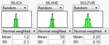
To show a common workflow with the Defect profiler, we use Tiretread.jmp with the specification limits from Table 8.1. We also give the following random specifications to the three factors.
Figure 8.15 Profiler
Select Defect Profiler to see the defect profiles. The curves, Means, and SDs will change from simulation to simulation, but will be relatively consistent.
Figure 8.16 Defect Profiler
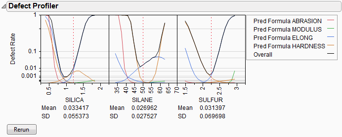
The black curve on each factor shows the defect rate if you could fix that factor at the x-axis value, but leave the other features random.
Look at the curve for SILICA. As its values vary, its defect rate goes from the lowest 0.001 at SILICA=0.95, quickly up to a defect rate of 1 at SILICA=0.4 or 1.8. However, SILICA is itself random. If you imagine integrating the density curve of SILICA with its defect profile curve, you could estimate the average defect rate 0.033, also shown as the Mean for SILICA. This is estimating the overall defect rate shown under the simulation histograms, but by numerically integrating, rather than by the overall simulation. The Means for the other factors are similar. The numbers are not exactly the same. However, we now also get an estimate of the standard deviation of the defect rate with respect to the variation in SILICA. This value (labeled SD) is 0.055. The standard deviation is intimately related to the sensitivity of the defect rate with respect to the distribution of that factor.
Looking at the SDs across the three factors, we see that the SD for SULFUR is higher than the SD for SILICA, which is in turn much higher than the SD for SILANE. This means that to improve the defect rate, improving the distribution in SULFUR should have the greatest effect. A distribution can be improved in three ways: changing its mean, changing its standard deviation, or by chopping off the distribution by rejecting parts that do not meet certain specification limits.
In order to visualize all these changes, there is another command in the Simulator red triangle menu, Defect Parametric Profile, which shows how single changes in the factor distribution parameters affect the defect rate.
Figure 8.17 Defect Parametric Profile
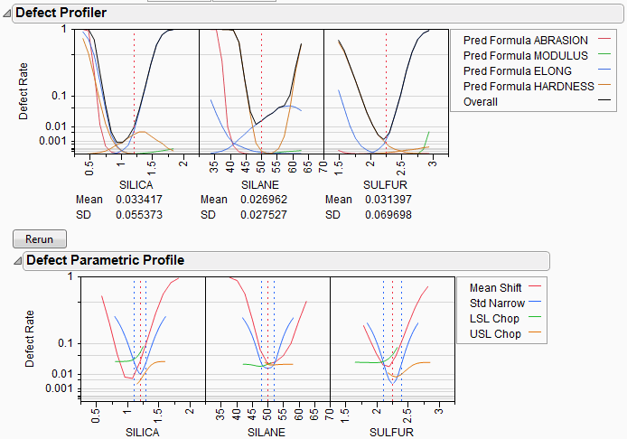
Let’s look closely at the SULFUR situation. You might need to enlarge the graph to see more detail.
First, note that the current defect rate (0.03) is represented in four ways corresponding to each of the four curves.
For the red curve, Mean Shift, the current rate is where the red solid line intersects the vertical red dotted line. The Mean Shift curve represents the change in overall defect rate by changing the mean of SULFUR. One opportunity to reduce the defect rate is to shift the mean slightly to the left. If you use the crosshair tool on this plot, you see that a mean shift reduces the defect rate to about 0.02.
For the blue curve, Std Narrow, the current rate represents where the solid blue line intersects the two dotted blue lines. The Std Narrow curves represent the change in defect rate by changing the standard deviation of the factor. The dotted blue lines represent one standard deviation below and above the current mean. The solid blue lines are drawn symmetrically around the center. At the center, the blue line typically reaches a minimum, representing the defect rate for a standard deviation of zero. That is, if we totally eliminate variation in SULFUR, the defect rate is still around 0.003. This is much better than 0.03. If you look at the other Defect parametric profile curves, you can see that this is better than reducing variation in the other factors, something that we suspected by the SD value for SULFUR.
For the green curve, LSL Chop, there are no interesting opportunities in this example, because the green curve is above current defect rates for the whole curve. This means that reducing the variation by rejecting parts with too-small values for SULFUR will not help.
For the orange curve, USL Chop, there are good opportunities. Reading the curve from the right, the curve starts out at the current defect rate (0.03), then as you start rejecting more parts by decreasing the USL for SULFUR, the defect rate improves. However, moving a spec limit to the center is equivalent to throwing away half the parts, which might not be a practical solution.
Looking at all the opportunities over all the factors, it now looks like there are two good options for a first move: change the mean of SILICA to about 1, or reduce the variation in SULFUR. Because it is generally easier in practice to change a process mean than process variation, the best first move is to change the mean of SILICA to 1.
Figure 8.18 Adjusting the Mean of Silica
After changing the mean of SILICA, all the defect curves become invalid and need to be rerun. After clicking Rerun, we get a new perspective on defect rates.
Figure 8.19 Adjusted Defect Rates
Now, the defect rate is down to about 0.004, much improved. Further reduction in the defect rate can occur by continued investigation of the parametric profiles, making changes to the distributions, and rerunning the simulations.
As the defect rate is decreased further, the mean defect rates across the factors become relatively less reliable. The accuracy could be improved by reducing the ranges of the factors in the Profiler a little so that it integrates the distributions better.
This level of fine-tuning is probably not practical, because the experiment that estimated the response surface is probably not at this high level of accuracy. Once the ranges have been refined, you might need to conduct another experiment focusing on the area that you know is closer to the optimum.
Stochastic Optimization Example
This example is adapted from Box and Draper (1987) and uses Stochastic Optimization.jmp. A chemical reaction converts chemical “A” into chemical “B”. The resulting amount of chemical “B” is a function of reaction time and reaction temperature. A longer time and hotter temperature result in a greater amount of “B”. But, a longer time and hotter temperature also result in some of chemical “B” getting converted to a third chemical “C”. What reaction time and reaction temperature will maximize the resulting amount of “B” and minimize the amount of “A” and “C”? Should the reaction be fast and hot, or slow and cool?
Figure 8.20 Chemical Reaction
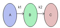
The goal is to maximize the resulting amount of chemical “B”. One approach is to conduct an experiment and fit a response surface model for reaction yield (amount of chemical “B”) as a function of time and temperature. But, due to well known chemical reaction models, based on the Arrhenius laws, the reaction yield can be directly computed. The column Yield contains the formula for yield. The formula is a function of Time (hours) and reaction rates k1 and k2. The reaction rates are a function of reaction Temperature (degrees Kelvin) and known physical constants θ1, θ2, θ3, θ4. Therefore, Yield is a function of Time and Temperature.
Figure 8.21 Formula for Yield
You can use the Profiler to find the maximum Yield. Open Stochastic Optimization.jmp and run the attached script called Profiler. Profiles of the response are generated as follows.
Figure 8.22 Profile of Yield
To maximize Yield use a desirability function. See the “Desirability Profiling and Optimization” in the “Profiler” chapter. One possible desirability function was incorporated in the script. To view the function choose Desirability Functions from the Prediction Profiler red triangle menu.
Figure 8.23 Prediction Profiler
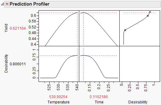
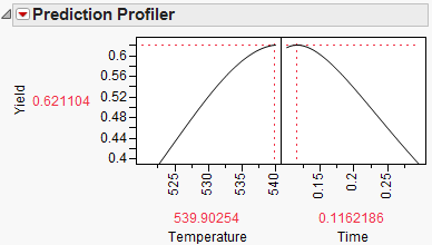
To maximize Yield, select Maximize Desirability from the Prediction Profiler red triangle menu. The Profiler then maximizes Yield and sets the graphs to the optimum value of Time and Temperature.
Figure 8.24 Yield Maximum
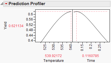
The maximum Yield is approximately 0.62 at a Time of 0.116 hours and Temperature of 539.92 degrees Kelvin, or hot and fast. [Your results might differ slightly due to random starting values in the optimization process. Optimization settings can be modified (made more stringent) by selecting Maximization Options from the Prediction Profiler red triangle menu. Decreasing the Covergence Tolerance will enable the solution to be reproducible.]
In a production environment, process inputs cannot always be controlled exactly. What happens to Yield if the inputs (Time and Temperature) have random variation? Furthermore, if Yield has a spec limit, what percent of batches will be out of spec and need to be discarded? The Simulator can help us investigate the variation and defect rate for Yield, given variation in Time and Temperature.
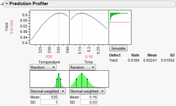
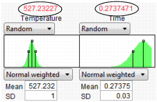
Select Simulator from the Prediction Profiler red triangle menu. As shown in Figure 8.25, fill in the factor parameters so that Temperature is Normal weighted with standard deviation of 1, and Time is Normal weighted with standard deviation of 0.03. The Mean parameters default to the current factor values. Change the number of runs to 15,000. Yield has a lower spec limit of 0.55, set as a column property, and shows on the chart as a red line. If it does not show by default, enter it by selecting Spec Limits on the Simulator red triangle menu.
Figure 8.25 Initial Simulator Settings
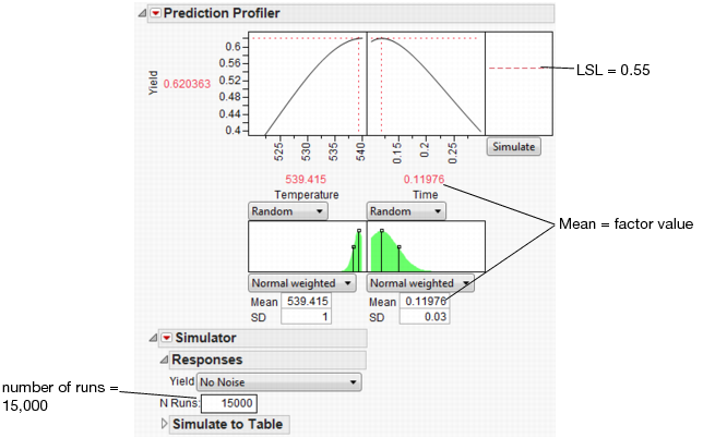
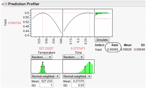
With the random variation set for the input factors, you are ready to run a simulation to study the resulting variation and defect rate for Yield. Click the Simulate button.
Figure 8.26 Simulation Results
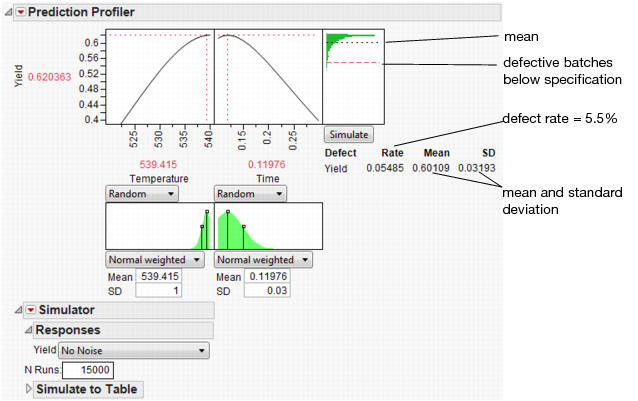
The predicted Yield is 0.62, but if the factors have the given variation, the average Yield is 0.60 with a standard deviation of 0.03.
The defect rate is about 5.5%, meaning that about 5.5% of batches are discarded. A defect rate this high is not acceptable.
What is the defect rate for other settings of Temperature and Time? Suppose you change the Temperature to 535, then set Time to the value that maximizes Yield? Enter settings as shown in Figure 8.27 then click Simulate.
Figure 8.27 Defect Rate for Temperature of 535
The defect rate decreases to about 1.8%, which is much better than 5.5%. So, what you see is that the fixed (no variability) settings that maximize Yield are not the same settings that minimize the defect rate in the presence of factor variation.
By running a Simulation Experiment you can find the settings of Temperature and Time that minimize the defect rate. To do this you simulate the defect rate at each point of a Temperature and Time design, then fit a predictive model for the defect rate and minimize it.
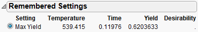
Before running the Simulation Experiment, save the factor settings that maximize Yield so you can reference them later. To do this, re-enter the factor settings (Mean and SD) from Figure 8.25 and select Factor Settings > Remember Settings from Prediction Profiler red triangle menu. A window prompts you to name the settings then click OK. The settings are appended to the report window.
Figure 8.28 Remembered Settings
Select Simulation Experiment from the Simulator red triangle menu. Enter 80 runs, and 1 to use the whole factor space in the experiment. A Latin Hypercube design with 80 design points is chosen within the specified factor space, and N Runs random draws are taken at each of the design points. The design point are the center of the random draws, and the shape and variance of the random draws coming from the factor distributions.
A table is created with the results of the experiment. The Overall Defect Rate is given at each design point. You can now fit a model that predicts the defect rate as a function of Temperature and Time. To do this, run the attached Guassian Process script and wait for the results. The results are shown below. Your results will be slightly different due to the random draws in the simulation.
Figure 8.29 Results of Gaussian Process Model Fit
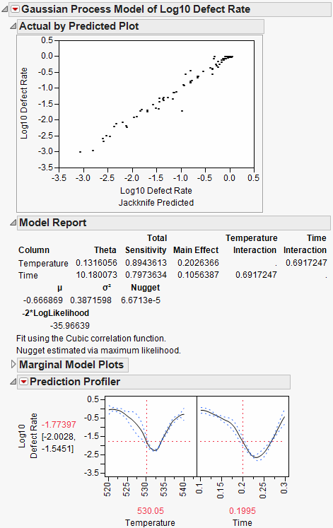
The Gaussian Process platform automatically starts the Prediction Profiler. The desirability function is already set up to minimize the defect rate. To find the settings of Temperature and Time that minimizes the defect rate, select Maximize Desirability from the Prediction Profiler red triangle menu.
Figure 8.30 Settings for Minimum Defect Rate
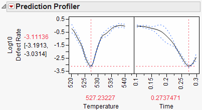
The settings that minimize the defect rate are approximately Temperature = 527 and Time = 0.27. Select Factor Settings > Copy Settings Script from the Prediction Profiler red triangle menu. Return to the original Profiler report window and select Factor Settings > Paste Settings Script. This sets Temperature and Time to those settings that minimize the defect rate. Use Remember Settings as before to save these new settings.
Figure 8.31 Minimum Defect Settings
With the new settings in place, click the Simulate button to estimate the defect rate at the new settings.
Figure 8.32 Lower Defect Rate
At the new settings the defect rate is 0.066%, much better than the 5.5% for the settings that maximize Yield. That is a reduction of about 100x. Recall the average Yield from the first settings is 0.60 and the new average is 0.59. The decrease in average Yield of 0.01 is very acceptable when the defect rate decreases by 100x.
Because we saved the settings using Remember Settings, we can easily compare the old and new settings. The Differences report summarizes the difference. Click the Remembered Settings radio buttons to view the profiler for each setting.
Figure 8.33 Settings Comparison
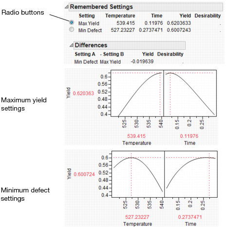
The chemist now knows what settings to use for a quality process. If the factors have no variation, the settings for maximum Yield are hot and fast. But, if the process inputs have variation similar to what we have simulated, the settings for maximum Yield produce a high defect rate. Therefore, to minimize the defect rate in the presence of factor variation, the settings should be cool and slow.
Statistical Details
This section contains statistical details for the Simulator profiler.
Normal Weighted Distribution
JMP uses the multivariate radial strata method for each factor that uses the Normal Weighted distribution. This seems to work better than a number of Importance Sampling methods, as a multivariate Normal Integrator accurate in the extreme tails.
First, define strata and calculate corresponding probabilities and weights. For d random factors, the strata are radial intervals as follows.
|
Strata Number
|
Inside Distance
|
Outside Distance
|
|
0
|
0
|
|
|
1
|
|
|
|
2
|
|
|
|
i
|
|
|
|
NStrata – 1
|
previous
|
|
The default number of strata is 12. To change the number of strata, a hidden command N Strata is available if you hold the Shift key down while clicking on the red triangle next to Simulator. Increase the sample size as needed to maintain an even number of strata.
For each simulation run:
1. Select a strata as mod(i – 1, NStrata) for run i.
2. Determine a random n-dimensional direction by scaling multivariate Normal (0,1) deviates to unit norm.
3. Determine a random distance using a chi-square quantile appropriate for the strata of a random uniform argument.
4. Scale the variates so that the norm is the random distance.
5. Scale and re-center the variates individually to be as specified for each factor.
The resulting factor distributions are multivariate normal with the appropriate means and standard deviations when estimated with the right weights. Note that you cannot use the Distribution standard deviation with weights, because it does not estimate the desired value. However, multiplying the weight by a large value, like 1012, and using that as a Freq value results in the correct standard deviation.
..................Content has been hidden....................
You can't read the all page of ebook, please click here login for view all page.