Excel Profiler Overview
The JMP Add-In for Excel uses the JMP Profiler to visualize models (or formulas) stored in Excel worksheets. The Excel add-in is automatically installed when you install JMP. Profiling in the Excel Add-In is a two-step process:
1. Click the Create/Edit Model button (Excel 2007 through 2013) to enter information about the model that JMP needs. This needs to be done only once per model. For more information, click Help in the Create/Edit Model window.
2. Click the Run Model button (Excel 2007 through 2013) to launch the JMP Profiler and run the Excel model. For more information, see “Running the JMP Profiler”.
Note: The Preferences, Data Table, Graph Builder, and Distribution buttons are not needed to profile an Excel model. For more information about these features, see Using JMP.
Running the JMP Profiler
Once you create the model using the Excel Add-In, you can run it in the JMP Profiler. From the Excel Add-In, perform the following actions:
1. Click the Run Model button (Excel 2007 through 2013).
2. Select the model that you want to run.
3. Click Profile in JMP.
Note: To ensure that your original Excel spreadsheet is not altered, JMP runs a hidden copy of Excel in the background that controls all of the Profiler calculations.
Example of an Excel Model
An Excel model is one or more Excel formulas. Each formula must be a function of one or more other cells. This example uses the Demand.xls file, located within C:Program FilesSASJMP<version number>SamplesImport Data).
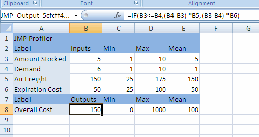
Figure 10.2 Demand Model in Excel

The formula is in cell B8, and is a calculation of the Overall Cost associated with having different amounts of product in stock. The formula can be seen in the Formula Bar, and is a function of four cells:
• Amount Stocked is the amount of product in stock.
• Demand is the customer demand for the product.
• Air Freight is the cost per unit to ship additional product by air when the demand exceeds the amount in stock.
• Expiration Cost is the cost per unit of disposing of unused product when the demand is less than the amount in stock.
The calculations of the formula are as follows:
• If Amount Stocked is less than Demand, then the company has to ship additional units, at a cost of (Demand-Amount Stocked) x Air Freight. For example, if the demand is 8, but the company has only 6 in stock, then it has to ship 8-6=2 units at a cost of 2x150=300.
• If Amount Stocked is greater than Demand, then the company has to dispose of unused product, at a cost of (Amount Stocked-Demand) x Expiration Cost. For example, if the demand is 5, but the company has 8 in stock, then it has to dispose of 8-5=3 units at a cost of 3x50=150.
• If Amount Stocked is equal to Demand, then there is no shipping cost or disposal cost.
• There is never both a shipping cost and a disposal cost at the same time.
Using the model in Excel, you can get the cost for only a given set of inputs at once. It is difficult to visualize how changing the value of one input affects the output. You can choose a different combination of the inputs to see how the cost is affected, but doing so for many combinations can take a long time.
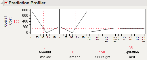
Use the JMP Profiler to simultaneously see the effect of all inputs on the output. Also, you can quickly simulate a range of input combinations to see the resulting range of output values.
Figure 10.3 Example of the Profiler Using Excel Models

Using Linear Constraints
Within the JMP Profiler, you can alter the linear constraints in order to restrict the model input values. You are prompted to save the constraints to the Excel workbook. After constraints are saved to the Excel workbook, whenever the model is profiled from the Excel Add-In, the constraints are incorporated.
1. From the red triangle menu next to Prediction Profiler, select Alter Linear Constraints.
2. Click Add Constraint.
3. Type in the constraining values.
4. Click OK.
5. From the red triangle menu next to Prediction Profiler, select Save Linear Constraints.
You are prompted to save the constraints to the Excel workbook.
6. Click Yes.
Note: When you save the .xls file in Excel 2007, you might see a compatibility error. If so, click Continue to save the file.
The workbook opens in Excel. When you run the model, the constraints are reflected in the JMP Profiler. For more information about linear constraints, see “Linear Constraints” in the “Profiler” chapter.
Tip: To delete a linear constraint, set all constraint values to zero.
Resolution of Profile Lines
The Default N Levels option on the red triangle menu next to Prediction Profiler affects the resolution of the profile lines. Note the following information:
• This option defaults to 17 when the Profiler runs a model stored in Excel.
• This option defaults to 41 when the model is stored directly in JMP.
If the same model is stored in both Excel and JMP, then the profile lines can appear differently when the models are profiled. Increasing this value causes the Excel Profiler to run slower.
Using the Excel Profiler from JMP
Once an Excel file has the model inputs and outputs defined, you can profile the model from within JMP.
1. Select Graph > Excel Profiler.
2. Locate the Excel file containing the model and then click Open.
3. If the Excel file contains multiple models, you are prompted to select the model that you want to profile.
Note that the Excel Profiler is also scriptable, as follows:
Excel Profiler( "path to workbook", <"model name"> ) ;
If more than one model exists, and no model is specified, a window with the list of available models appears. For more information about scripting the Excel Profiler, see the Scripting Guide.
Statistical Details
Normal Weighted Distribution
JMP uses the multivariate radial strata method for each factor that uses the Normal Weighted distribution. This seems to work better than a number of Importance Sampling methods, as a multivariate Normal Integrator accurate in the extreme tails.
First, define strata and calculate corresponding probabilities and weights. For d random factors, the strata are radial intervals as follows.
|
Strata Number
|
Inside Distance
|
Outside Distance
|
|
0
|
0
|
|
|
1
|
|
|
|
2
|
|
|
|
i
|
|
|
|
NStrata – 1
|
previous
|
|
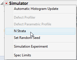
The default number of strata is 12. To change the number of strata, a hidden command N Strata is available if you hold the Shift key down while clicking on the red triangle next to Simulator.
Figure 10.4 Showing the N Strata Menu Option

Increase the sample size as needed to maintain an even number of strata.
For each simulation run,
1. Select a strata as mod(i – 1, NStrata) for run i.
2. Determine a random n-dimensional direction by scaling multivariate Normal (0,1) deviates to unit norm.
3. Determine a random distance using a chi-square quantile appropriate for the strata of a random uniform argument.
4. Scale the variates so that the norm is the random distance.
5. Scale and re-center the variates individually to be as specified for each factor.
The resulting factor distributions are multivariate normal with the appropriate means and standard deviations when estimated with the right weights. Note that you cannot use the Distribution standard deviation with weights, because it does not estimate the desired value. However, multiplying the weight by a large value, like 1012, and using that as a Freq value results in the correct standard deviation.
..................Content has been hidden....................
You can't read the all page of ebook, please click here login for view all page.
