Chapter 10: Processing LLVM IR
In the previous chapter, we learned about PassManager and AnalysisManager in LLVM. We went through some tutorials for developing an LLVM pass and how to retrieve program analysis data via AnalysisManager. The knowledge and skills we acquired help to build the foundation for developers to create composable building blocks for code transformation and program analysis.
In this chapter, we are going to focus on the methodology of processing LLVM IR. LLVM IR is a target-independent intermediate representation for program analysis and compiler transformation. You can think of LLVM IR as an alternative form of the code you want to optimize and compile. However, different from the C/C++ code you're familiar with, LLVM IR describes the program in a different way – we will give you a more concrete idea later. The majority of the magic that's done by LLVM that makes the input program faster or smaller after the compilation process is performed on LLVM IR. Recall that in the previous chapter, Chapter 9, Working with PassManager and AnalysisManager, we described how different passes are organized in a pipeline fashion – that was the high-level structure of how LLVM transforms the input code. In this chapter, we are going to show you the fine-grained details of how to modify LLVM IR in an efficient way.
Although the most straightforward and visual way to view LLVM IR is by its textual representation, LLVM provides libraries that contain a set of powerful modern C++ APIs to interface with the IR. These APIs can inspect the in-memory representation of LLVM IR and help us manipulate it, which effectively changes the target program we are compiling. These LLVM IR libraries can be embedded in a wide variety of applications, allowing developers to transform and analyze their target source code with ease.
LLVM APIs for different programming languages
Officially, LLVM only supports APIs for two languages: C and C++. Between them, C++ is the most feature-complete and update to date, but it also has the most unstable interface – it might be changed at any time without backward compatibility. On the other hand, C APIs have stable interfaces but come at the cost of lagging behind new feature updates, or even keeping certain features absent. The API bindings for OCaml, Go, and Python are in the source tree as community-driven projects.
We will try to guide you with generally applicable learning blocks driven by commonly seen topics and tasks that are supported by many realistic examples. Here is the list of topics we'll cover in this chapter:
- Learning LLVM IR basics
- Working with values and instructions
- Working with loops
We will start by introducing LLVM IR. Then, we will learn about two of the most essential elements in LLVM IR – values and instructions. Finally, we'll end this chapter by looking at loops in LLVM – a more advanced topic that is crucial for working on performance-sensitive applications.
Technical requirements
The tools we'll need in this chapter are the opt command-line utility and clang. Please build them using the following command:
$ ninja opt clang
Most of the code in this chapter can be implemented inside LLVM pass – and the pass plugin – as introduced in Chapter 9, Working with PassManager and AnalysisManager.
In addition, please install the Graphviz tool. You can consult the following page for an installation guide for your system: https://graphviz.org/download. On Ubuntu, for instance, you can install that package via the following command:
$ sudo apt install graphviz
We will use a command-line tool – the dot command – provided by Graphviz to visualize the control flow of a function.
The code example mentioned in this chapter can be implemented inside LLVM pass, if not specified otherwise.
Learning LLVM IR basics
LLVM IR is an alternative form of the program you want to optimize and compile. It is, however, structured differently from normal programming languages such as C/C++. LLVM IR is organized in a hierarchical fashion. The levels in this hierarchy – counting from the top – are Module, function, basic block, and instruction. The following diagram shows their structure:

Figure 10.1 – Hierarchy structure of LLVM IR
A module represents a translation unit – usually a source file. Each module can contain multiple functions (or global variables). Each contains a list of basic blocks where each of the basic blocks contains a list of instructions.
Quick refresher – basic block
A basic block represents a list of instructions with only one entry and one exit point. In other words, if a basic block is executed, the control flow is guaranteed to walk through every instruction in the block.
Knowing the high-level structure of LLVM IR, let's look at one of the LLVM IR examples. Let's say we have the following C code, foo.c:
int foo(int a, int b) {
return a > 0? a – b : a + b;
}
We can use the following clang command to generate its textual LLVM IR counterpart:
$ clang -emit-llvm -S foo.c
The result will be put in the foo.ll file. The following diagram shows part of its content, with annotations for the corresponding IR unit:
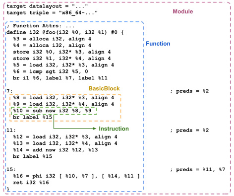
Figure 10.2 – Part of the content in foo.ll, annotated with the corresponding IR unit
In textual form, an instruction is usually presented in the following format:
<result> = <operator / op-code> <type>, [operand1, operand2, …]
For instance, let's assume we have the following instruction:
%12 = load i32, i32* %3
Here, %12 is the result value, load is the op-code, i32 is the data type of this instruction, and %3 is the only operand.
In addition to the textual representation, nearly every component in LLVM IR has a C++ class counterpart with the same name. For instance, a function and a basic block are simply represented by Function and the BasicBlock C++ class, respectively.
Different kinds of instructions are represented by classes that are all derived from the Instruction class. For example, the BinaryOperator class represents a binary operation instruction, while ReturnInst class represents a return statement. We will look at Instruction and its child classes in more detail later.
The hierarchy depicted in Figure 10.1 is the concrete structure of LLVM IR. That is, this is how they are stored in memory. On top of that, LLVM also provides other logical structures to view the relationships of different IR units. They are usually evaluated from the concrete structures and stored as auxiliary data structures or treated as analysis results. Here are some of the most important ones in LLVM:
- Control Flow Graph (CFG): This is a graph structure that's organized into basic blocks to show their control flow relations. The vertices in this graph represent basic blocks, while the edges represent a single control flow transfer.
- Loop: This represents the loop we are familiar with, which consists of multiple basic blocks that have at least one back edge – a control flow edge that goes back to its parent or ancestor vertices. We will look at this in more detail in the last section of this chapter, the Working with loops section.
- Call graph: Similar to CFG, the call graph also shows control flow transfers, but the vertices become individual functions and the edges become function call relations.
In the next section, we are going to learn how to iterate through different IR units in both concrete and logical structures.
Iterating different IR units
Iterating IR units – such as basic blocks or instructions – are essential to LLVM IR development. It is usually one of the first steps we must complete in many transformation or analysis algorithms – scanning through the whole code and finding an interesting area in order to apply certain measurements. In this section, we are going to learn about the practical aspects of iterating different IR units. We will cover the following topics:
- Iterating instructions
- Iterating basic blocks
- Iterating the call graph
- Learning the GraphTraits
Let's start by discussing how to iterate instructions.
Iterating instructions
An instruction is one of the most basic elements in LLVM IR. It usually represents a single action in the program, such as an arithmetic operation or a function call. Walking through all the instructions in a single basic block or function is the cornerstone of most program analyses and compiler optimizations.
To iterate through all the instructions in a basic block, you just need to use a simple for-each loop over the block:
// `BB` has the type of `BasicBlock&`
for (Instruction &I : BB) {
// Work on `I`
}
We can iterate through all the instructions in a function in two ways. First, we can iterate over all the basic blocks in the function before visiting the instructions. Here is an example:
// `F` has the type of `Function&`
for (BasicBlock &BB : F) {
for (Instruction &I : BB) {
// Work on `I`
}
}
Second, you can leverage a utility called inst_iterator. Here is an example:
#include "llvm/IR/InstIterator.h"
…
// `F` has the type of `Function&`
for (Instruction &I : instructions(F)) {
// Work on `I`
}
Using the preceding code, you can retrieve all the instructions in this function.
Instruction visitor
There are many cases where we want to apply different treatments to different types of instructions in a basic block or function. For example, let's assume we have the following code:
for (Instruction &I : instructions(F)) {
switch (I.getOpcode()) {
case Instruction::BinaryOperator:
// this instruction is a binary operator like `add` or `sub`
break;
case Instruction::Return:
// this is a return instruction
break;
…
}
}
Recall that different kinds of instructions are modeled by (different) classes derived from Instruction. Therefore, an Instruction instance can represent any of them. The getOpcode method shown in the preceding snippet can give you a unique token – namely, Instruction::BinaryOperator and Instruction::Return in the given code – that tells you about the underlying class. However, if we want to work on the derived class ( ReturnInst, in this case) instance rather than the "raw" Instruction, we need to do some type casting.
LLVM provides a better way to implement this kind of visiting pattern –InstVisitor. InstVisitor is a class where each of its member methods is a callback function for a specific instruction type. You can define your own callbacks after inheriting from the InstVisitor class. For instance, check out the following code snippet:
#include "llvm/IR/InstVisitor.h"
class MyInstVisitor : public InstVisitor<MyInstVisitor> {
void visitBinaryOperator(BinaryOperator &BOp) {
// Work on binary operator instruction
…
}
void visitReturnInst(ReturnInst &RI) {
// Work on return instruction
…
}
};
Each visitXXX method shown here is a callback function for a specific instruction type. Note that we are not overriding each of these methods (there was no override keyword attached to the method). Also, instead of defining callbacks for all the instruction types, InstVisitor allows you to only define those that we are interested in.
Once MyInstVisitor has been defined, we can simply create an instance of it and invoke the visit method to launch the visiting process. Let's take the following code as an example:
// `F` has the type of `Function&`
MyInstVisitor Visitor;
Visitor.visit(F);
There are also visit methods for Instruction, BasicBlock, and Module.
Ordering basic blocks and instructions
All the skills we've introduced in this section assume that the ordering of basic blocks or even instructions to visit is not your primary concern. However, it is important to know that Function doesn't store or iterate its enclosing BasicBlock instances in a particular linear order. We will show you how to iterate through all the basic blocks in various meaningful orders shortly.
With that, you've learned several ways to iterate instructions from a basic block or a function. Now, let's learn how to iterate basic blocks in a function.
Iterating basic blocks
In the previous section, we learned how to iterate basic blocks of a function using a simple for loop. However, developers can only receive basic blocks in an arbitrary order in this way – that ordering gave you neither the execution order nor the control flow information among the blocks. In this section, we will show you how to iterate basic blocks in a more meaningful way.
Basic blocks are important elements for expressing the control flow of a function, which can be represented by a directed graph – namely, the CFG. To give you a concrete idea of what a typical CFG looks like, we can leverage one of the features in the opt tool. Assuming you have an LLVM IR file, foo.ll, you can use the following command to print out the CFG of each function in Graphviz format:
$ opt -dot-cfg -disable-output foo.ll
This command will generate one .dot file for each function in foo.ll.
The .dot File might be hidden
The filename of the CFG .dot file for each function usually starts with a dot character ('.'). On Linux/Unix systems, this effectively hides the file from the normal ls command. So, use the ls -a command to show those files instead.
Each .dot file contains the Graphviz representation of that function's CFG. Graphviz is a general and textual format for expressing graphs. People usually convert a .dot file into other (image) formats before studying it. For instance, using the following command, you can convert a .dot file into a PNG image file that visually shows the graph:
$ dot -Tpng foo.cfg.dot > foo.cfg.png
The following diagram shows two examples:

Figure 10.3 – Left: CFG for a function containing branches; right: CFG for a function containing a loop
The left-hand side of the preceding diagram shows a CFG for a function containing several branches; the right-hand side shows a CFG for a function containing a single loop.
Now, we know that basic blocks are organized as a directed graph – namely, the CFG. Can we iterate this CFG so that it follows the edges and nodes? LLVM answers this question by providing utilities for iterating a graph in four different ways: topological order, depth first (essentially doing DFS), breadth first (essentially doing BFS), and Strongly Connected Components (SCCs). We are going to learn how to use each of these utilities in the following subsections.
Let's start with topological order traversal.
Topological order traversal
Topological ordering is a simple linear ordering that guarantees that for each node in the graph, it will only be visited after we've visited all of its parent (predecessor) nodes. LLVM provides po_iterator and some other utility functions to implement reversed topological ordering (reversed topological ordering is easier to implement) on the CFG. The following snippet gives an example of using po_iterator:
#include "llvm/ADT/PostOrderIterator.h"
#include "llvm/IR/CFG.h"
// `F` has the type of `Function*`
for (BasicBlock *BB : post_order(F)) {
BB->printAsOperand(errs());
errs() << " ";
}
The post_order function is just a helper function to create an iteration range of po_iterator. Note that the llvm/IR/CFG.h header is necessary to make po_iterator work on Function and BasicBlock.
If we apply the preceding code to the function containing branches in the preceding diagram, we'll get the following command-line output:
label %12
label %9
label %5
label %7
label %3
label %10
label %1
Alternatively, you can traverse from a specific basic block using nearly the same syntax; for instance:
// `F` has the type of `Function*`
BasicBlock &EntryBB = F->getEntryBlock();
for (BasicBlock *BB : post_order(&EntryBB)) {
BB->printAsOperand(errs());
errs() << " ";
}
The preceding snippet will give you the same result as the previous one since it's traveling from the entry block. You're free to traverse from the arbitrary block, though.
Depth-first and breadth-first traversal
DFS and BFS are two of the most famous and iconic algorithms for visiting topological structures such as a graph or a tree. For each node in a tree or a graph, DFS will always try to visit its child nodes before visiting other nodes that share the same parents (that is, the sibling nodes). On the other hand, BFS will traverse all the sibling nodes before moving to its child nodes.
LLVM provides df_iterator and bf_iterator (and some other utility functions) to implement depth-first and breadth-first ordering, respectively. Since their usages are nearly identical, we are only going to demonstrate df_iterator here:
#include "llvm/ADT/DepthFirstIterator.h"
#include "llvm/IR/CFG.h"
// `F` has the type of `Function*`
for (BasicBlock *BB : depth_first(F)) {
BB->printAsOperand(errs());
errs() << " ";
}
Similar to po_iterator and post_order, depth_first is just a utility function for creating an iteration range of df_iterator. To use bf_iterator, simply replace depth_first with breadth_first. If you apply the preceding code to the containing branches in the preceding diagram, it will give you the following command-line output:
label %1
label %3
label %5
label %9
label %12
label %7
label %10
When using bf_iterator/breadth_first, we will get the following command-line output for the same example:
label %1
label %3
label %10
label %5
label %7
label %12
label %9
df_iterator and bf_iterator can also be used with BasicBlock, in the same way as po_iterator shown previously.
SSC traversal
An SCC represents a subgraph where every enclosing node can be reached from every other node. In the context of CFG, it is useful to traverse CFG with loops.
The basic block traversal methods we introduced earlier are useful tools to reason about the control flow in a function. For a loop-free function, these methods give you a linear view that closely reflects the execution orders of enclosing basic blocks. However, for a function that contains loops, these (linear) traversal methods cannot show the cyclic execution flow that's created by the loops.
Recurring control flow
Loops are not the only programming constructs that create recurring control flows within a function. A few other directives – the goto syntax in C/C++, for example – will also introduce a recurring control flow. However, those corner cases will make analyzing the control flow more difficult (which is one of the reasons you shouldn't use goto in your code), so when we are talking about recurring control flows, we are only referring to loops.
Using scc_iterator in LLVM, we can traverse strongly connected basic blocks in a CFG. With this information, we can quickly spot a recurring control flow, which is crucial for some analysis and program transformation tasks. For example, we need to know the back edges and recurring basic blocks in order to accurately propagate the branch probability data along the control flow edges.
Here is an example of using scc_iterator:
#include "llvm/ADT/SCCIterator.h"
#include "llvm/IR/CFG.h"
// `F` has the type of `Function*`
for (auto SCCI = scc_begin(&F); !SCCI.isAtEnd(); ++SCCI) {
const std::vector<BasicBlock*> &SCC = *SCCI;
for (auto *BB : SCC) {
BB->printAsOperand(errs());
errs() << " ";
}
errs() << "==== ";
}
Different from the previous traversal methods, scc_iterator doesn't provide a handy range-style iteration. Instead, you need to create a scc_iterator instance using scc_begin and do manual increments. More importantly, you should use the isAtEnd method to check the exit condition, rather than doing a comparison with the "end" iterator like we usually do with C++ STL containers. A vector of BasicBlock can be dereferenced from a single scc_iterator. These BasicBlock instances are the basic blocks within a SCC. The ordering among these SCC instances is roughly the same as in the reversed topological order – namely, the post ordering we saw earlier.
If you run the preceding code over the function that contains a loop in the preceding diagram, it gives you the following command-line output:
label %6
====
label %4
label %2
====
label %1
====
This shows that basic blocks %4 and %2 are in the same SCC.
With that, you've learned how to iterate basic blocks within a function in different ways. In the next section, we are going to learn how to iterate functions within a module by following the call graph.
Iterating the call graph
A call graph is a direct graph that represents the function call relationships in a module. It plays an important role in inter-procedural code transformation and analysis, namely, analyzing or optimizing code across multiple functions. A famous optimization called function inlining is an example of this.
Before we dive into the details of iterating nodes in the call graph, let's take a look at how to build a call graph. LLVM uses the CallGraph class to represent the call graph of a single Module. The following sample code uses a pass module to build a CallGraph:
#include "llvm/Analysis/CallGraph.h"
struct SimpleIPO : public PassInfoMixin<SimpleIPO> {
PreservedAnalyses run(Module &M, ModuleAnalysisManager &MAM) {
CallGraph CG(M);
for (auto &Node : CG) {
// Print function name
if (Node.first)
errs() << Node.first->getName() << " ";
}
return PreservedAnalysis::all();
}
};
This snippet built a CallGraph instance before iterating through all the enclosing functions and printing their names.
Just like Module and Function, CallGraph only provides the most basic way to enumerate all its enclosing components. So, how do we traverse CallGraph in different ways – for instance, by using SCC – as we saw in the previous section? The answer to this is surprisingly simple: in the exact same way – using the same set of APIs and the same usages.
The secret behind this is a thing called GraphTraits.
Learning about GraphTraits
GraphTraits is a class designed to provide an abstract interface over various different graphs in LLVM – CFG and call graph, to name a few. It allows other LLVM components – analyses, transformations, or iterator utilities, as we saw in the previous section – to build their works independently of the underlying graphs. Instead of asking every graph in LLVM to inherit from GraphTraits and implement the required functions, GraphTraits takes quite a different approach by using template specialization.
Let's say that you have written a simple C++ class that has a template argument that accepts arbitrary types, as shown here:
template <typename T>
struct Distance {
static T compute(T &PointA, T &PointB) {
return PointA – PointB;
}
};
This C++ class will compute the distance between two points upon calling the Distance::compute method. The types of those points are parameterized by the T template argument.
If T is a numeric type such as int or float, everything will be fine. However, if T is a struct of a class, like the one here, then the default compute method implementation will not be able to compile:
Distance<int>::compute(94, 87); // Success
…
struct SimplePoint {
float X, Y;
};
SimplePoint A, B;
Distance<SimplePoint>::compute(A, B); // Compilation Error
To solve this issue, you can either implement a subtract operator for SimplePoint, or you can use template specialization, as shown here:
// After the original declaration of struct Distance…
template<>
struct Distance<SimplePoint> {
SimplePoint compute(SimplePoint &A, SimplePoint &B) {
return std::sqrt(std::pow(A.X – B.X, 2),…);
}
};
…
SimplePoint A, B;
Distance<SimplePoint>::compute(A, B); // Success
Distance<SimplePoint> in the previous code describes what Distance<T> looks like when T is equal to SimplePoint. You can think of the original Distance<T> as some kind of interface and Distance<SimplePoint> being one of its implementations. But be aware that the compute method in Distance<SimplePoint> is not an override method of the original compute in Distance<T>. This is different from normal class inheritance (and virtual methods).
GraphTraits in LLVM is a template class that provides an interface for various graph algorithms, such as df_iterator and scc_iterator, as we saw previously. Every graph in LLVM will implement this interface via template specialization. For instance, the following GraphTraits specialization is used for modeling the CFG of a function:
template<>
struct GraphTraits<Function*> {…}
Inside the body of GraphTraits<Function*>, there are several (static) methods and typedef statements that implement the required interface. For example, nodes_iterator is the type that's used for iterating over all the vertices in CFG, while nodes_begin provides you with the entry/starting node of this CFG:
template<>
struct GraphTraits<Function*> {
typedef pointer_iterator<Function::iterator> nodes_iterator;
static node_iterator nodes_begin(Function *F) {
return nodes_iterator(F->begin());
}
…
};
In this case, nodes_iterator is basically Function::iterator. nodes_begin simply returns the first basic block in the function (via an iterator). If we look at GraphTraits for CallGraph, it has completely different implementations of nodes_iterator and nodes_begin:
template<>
struct GraphTraits<CallGraph*> {
typedef mapped_iterator<CallGraph::iterator,
decltype(&CGGetValuePtr)> nodes_iterator;
static node_iterator nodes_begin(CallGraph *CG) {
return nodes_iterator(CG->begin(), &CGGetValuePtr);
}
};
When developers are implementing a new graph algorithm, instead of hardcoding it for each kind of graph in LLVM, they can build their algorithms by using GraphTraits as an interface to access the key properties of arbitrary graphs.
For example, let's say we want to create a new graph algorithm, find_tail, which finds the first node in the graph that has no child nodes. Here is the skeleton of find_tail:
template<class GraphTy,
typename GT = GraphTraits<GraphTy>>
auto find_tail(GraphTy G) {
for(auto NI = GT::nodes_begin(G); NI != GT::nodes_end(G); ++NI) {
// A node in this graph
auto Node = *NI;
// Child iterator for this particular node
auto ChildIt = GT::child_begin(Node);
auto ChildItEnd = GT::child_end(Node);
if (ChildIt == ChildItEnd)
// No child nodes
return Node;
}
…
}
With the help of this template and GraphTraits, we can reuse this function on Function, CallGraph, or any kind of graph in LLVM; for instance:
// `F` has the type of `Function*`
BasicBlock *TailBB = find_tail(F);
// `CG` has the type of `CallGraph*`
CallGraphNode *TailCGN = find_tail(CG);
In short, GraphTraits generalizes algorithms – such as df_iterator and scc_iterator, as we saw previously – in LLVM to arbitrary graphs using the template specialization technique. This is a clean and efficient way to define interfaces for reusable components.
In this section, we learned the hierarchy structure of LLVM IR and how to iterate different IR units – either concrete or logical units, such as CFGs. We also learned the important role of GraphTraits for encapsulating different graphs – CFGs and call graphs, to name a few – and exposed a common interface to various algorithms in LLVM, thus making those algorithms more concise and reusable.
In the next section, we will learn about how values are represented in LLVM, which describes a picture of how different LLVM IR components are associated with each other. In addition, we will learn about the correct and efficient way to manipulate and update values in LLVM.
Working with values and instructions
In LLVM, a value is a unique construct – not only does it represent values stored in variables, but it also models a wide range of concepts from constants, global variables, individual instructions, and even basic blocks. In other words, it is one of the foundations of LLVM IR.
The concept of value is especially important for instructions as it directly interacts with values in the IR. Therefore, in this section, we will put them into the same discussion. We are going to see how values work in LLVM IR and how values are associated with instructions. On top of that, we are going to learn how to create and insert new instructions, as well as how to update them.
To learn how to use values in LLVM IR, we must understand the important theory behind this system, which dictates the behavior and the format of LLVM instructions – the Single Static Assignment (SSA) form.
Understanding SSA
SSA is a way of structuring and designing IR to make program analysis and compiler transformation easier to perform. In SSA, a variable (in the IR) will only be assigned a value exactly once. This means that we cannot manipulate a variable like this:
// the following code is NOT in SSA form
x = 94;
x = 87; // `x` is assigned the second time, not SSA!
Although a variable can only be assigned once, it can be used multiple times in arbitrary instructions. For instance, check out the following code:
x = 94;
y = x + 4; // first time `x` is used
z = x + 2; // second time `x` is used
You might be wondering how normal C/C++ code – which is clearly not in SSA form – gets transformed into an SSA form of IR, such as LLVM. While there is a whole class of different algorithms and research papers that answer this question, which we are not going to cover here, most of the simple C/C++ code can be transformed using trivial techniques such as renaming. For instance, let's say we have the following (non-SSA) C code:
x = 94;
x = x * y; // `x` is assigned more than once, not SSA!
x = x + 5;
Here, we can rename x in the first assignment with something like x0 and x on the left-hand side of the second and third assignments with alternative names such as x1 and x2, respectively:
x0 = 94;
x1 = x0 * y;
x2 = x1 + 5;
With these simple measurements, we can obtain the SSA form of our original code with the same behavior.
To have a more comprehensive understanding of SSA, we must change our way of thinking about what instructions look like in a program. In imperative programming languages such as C/C++, we often treat each statement (instruction) as an action. For instance, in the following diagram, on the left-hand side, the first line represents an action that "assigns 94 to variable x" where the second line means "do some multiplication using x and y before storing the result in the x variable":
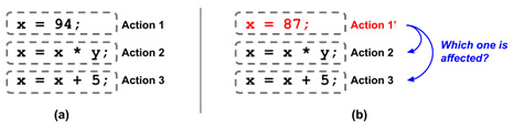
Figure 10.4 – Thinking instructions as "actions"
These interpretations sound intuitive. However, things get tricky when we make some transformations – which is, of course, a common thing in a compiler – on these instructions. In the preceding diagram, on the right-hand side, when the first instruction becomes x = 87, we don't know if this modification affects other instructions. If it does, we are not sure which one of these gets affected. This information not only tells us whether there are other potential opportunities to optimize, but it is also a crucial factor for the correctness of compiler transformation – after all, no one wants a compiler that will break your code when optimization is enabled. What's worse, let's say we are inspecting the x variable on the right-hand side of Action 3. We are interested in the last few instructions that modify this x. Here, we have no choice but to list all the instructions that have x on their left-hand side (that is, using x as the destination), which is pretty inefficient.
Instead of looking at the action aspect of an instruction, we can focus on the data that's generated by an instruction and get a clear picture of the provenance of each instruction – that is, the region that can be reached by its resulting value. Furthermore, we can easily find out the origins of arbitrary variables/values. The following diagram illustrates this advantage:

Figure 10.5 – SSA highlighting the dataflow among instructions
In other words, SSA highlights the dataflow in a program so that the compiler will have an easier time tracking, analyzing, and modify the instructions.
Instructions in LLVM are organized in SSA form. This means we are more interested in the value, or the data flow generated by an instruction, rather than which variable it stores the result in. Since each instruction in LLVM IR can only produce a single result value, an Instruction object – recall that Instruction is the C++ class that represents an instruction in LLVM IR – also represents its result value. To be more specific, the concept of value in LLVM IR is represented by a C++ class called Value. Instruction is one of its child classes. This means that given an Instruction object, we can, of course, cast it to a Value object. That particular Value object is effectively the result of that Instruction:
// let's say `I` represents an instruction `x = a + b`
Instruction *I = …;
Value *V = I; // `V` effectively represents the value `x`
This is one of the most important things to know in order to work with LLVM IR, especially to use most of its APIs.
While the Instruction object represents its own result value, it also has operands that are served as inputs to the instruction. Guess what? We are also using Value objects as operands. For example, let's assume we have the following code:
Instruction *BinI = BinaryOperator::Create(Instruction::Add,…);
Instruction *RetI = ReturnInst::Create(…, BinI, …);
The preceding snippet is basically creating an arithmetic addition instruction (represented by BinaryOperator), whose result value will be the operand of another return instruction. The resulting IR is equivalent to the following C/C++ code:
x = a + b;
return x;
In addition to Instruction, Constant (the C++ class for different kinds of constant values), GlobalVariable (the C++ class for global variables), and BasicBlock are all subclasses of Value. This means that they're also organized in SSA form and that you can use them as the operands for an Instruction.
Now, you know what SSA is and learned what impact it has on the design of LLVM IR. In the next section, we are going to discuss how to modify and update values in LLVM IR.
Working with values
SSA makes us focus on the data flow among instructions. Since we have a clear view of how values go from one instruction to the other, it's easy to replace the usage of certain values in an instruction. But how is the concept of "value usage" represented in LLVM? The following diagram shows two important C++ classes that answer this question – User and Use:
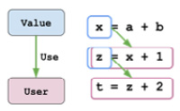
Figure 10.6 – The relationship between Value, User, and Use
As we can see, User represents the concept of an IR instance (for example, an Instruction) that uses a certain Value. Furthermore, LLVM uses another class, Use, to model the edge between Value and User. Recall that Instruction is a child class of Value – which represents the result that's generated by this instruction. In fact, Instruction is also derived from User, since almost all instructions take at least one operand.
A User might be pointed to by multiple Use instances, which means it uses many Value instances. You can use value_op_iterator provided by User to check out each of these Value instances; for example:
// `Usr` has the type of `User*`
for (Value *V : Usr->operand_values()) {
// Working with `V`
}
Again, operand_values is just a utility function to generate a value_op_iterator range.
Here is an example of why we want to iterate through all the User instances of a Value: imagine we are analyzing a program where one of its Function instances will return sensitive information – let's say, a get_password function. Our goal is to ensure that whenever get_password is called within a Function, its returned value (sensitive information) won't be leaked via another function call. For example, we want to detect the following pattern and raise an alarm:
void vulnerable() {
v = get_password();
…
bar(v); // WARNING: sensitive information leak to `bar`!
}
One of the most naïve ways to implement this analysis is by inspecting all User instances of the sensitive Value. Here is some example code:
User *find_leakage(CallInst *GetPWDCall) {
for (auto *Usr : GetPWDCall->users()) {
if (isa<CallInst>(Usr)) {
return Usr;
}
}
…
}
The find_leackage function takes a CallInst argument – which represents a get_password function call – and returns any User instance that uses the Value instance that's returned from that get_password call.
A Value instance can be used by multiple different User instances. So, similarly, we can iterate through all of them using the following snippet:
// `V` has the type of `Value*`
for (User *Usr : V->users()) {
// Working with `Usr`
}
With that, you've learned how to inspect the User instance of a Value, or the Value instance that's used by the current User. In addition, when we're developing a compiler transformation, it is pretty common to change the Value instance that's used by a User to another one. LLVM provides some handy utilities to do this.
First, the Value::replaceAllUsesWith method can, as its name suggests, tell all of its User instances to use another Value instead of it. The following diagram illustrates its effect:
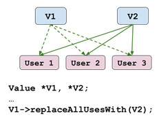
Figure 10.7 – Effect of Value::replaceAllUsesWith
This method is really useful when you're replacing an Instruction with another Instruction. Using the preceding diagram to explain this, V1 is the original Instruction and V2 is the new one.
Another utility function that does a similar thing is User::replaceUsesOfWith(From,To). This method effectively scans through all of the operands in this User and replaces the usage of a specific Value (the From argument) with another Value (the To argument).
The skills you've learned in this section are some of the most fundamental tools for developing a program transformation in LLVM. In the next section, we will talk about how to create and modify instructions.
Working with instructions
Previously, we learned the basics of Value – including its relationship with Instruction – and the way to update Value instances under the framework of SSA. In this section, we are going to learn some more basic knowledge and skills that give you a better understanding of Instruction and help you modify Instruction instances in a correct and efficient way, which is the key to developing a successful compiler optimization.
Here is the list of topics we are going to cover in this section:
- Casting between different instruction types
- Inserting a new instruction
- Replacing an instruction
- Processing instructions in batches
Let's start by looking at different instruction types.
Casting between different instruction types
In the previous section, we learned about a useful utility called InstVisitor. The InstVisitor class helps you determine the underlying class of an Instruction instance. It also saves you the efforts of casting between different instruction types. However, we cannot always rely on InstVisitor for every task that involves type casting between Instruction and its derived classes. More generally speaking, we want a simpler solution for type casting between parent and child classes.
Now, you might be wondering, but C++ already provided this mechanism via the dynamic_cast directive, right? Here is an example of dynamic_cast:
class Parent {…};
class Child1 : public Parent {…};
class Child2 : public Parent {…};
void foo() {
Parent *P = new Child1();
Child1 *C = dynamic_cast<Child1*>(P); // OK
Child2 *O = dynamic_cast<Child2*>(P); // Error: bails out at // runtime
}
In the foo function used in the preceding code, we can see that in its second line, we can convert P into a Child1 instance because that is its underlying type. On the other hand, we cannot convert P into Child2 – the program will simply crash during runtime if we do so.
Indeed, dynamic_cast has the exact functionality we are looking for – more formally speaking, the Runtime Type Info (RTTI) feature – but it also comes with high overhead in terms of runtime performance. What's worse, the default implementation of RTTI in C++ is quite complex, making the resulting program difficult to optimize. Therefore, LLVM disables RTTI by default. Due to this, LLVM came up with its own system of runtime type casting that is much simpler and more efficient. In this section, we are going to talk about how to use it.
LLVM's casting framework provides three functions for dynamic type casting:
- isa<T>(val)
- cast<T>(val)
- dyn_cast<T>(val)
The first function, isa<T> – pronounced "is-a" – checks if the val pointer type can be cast to a pointer of the T type. Here is an example:
// `I` has the type of `Instruction*`
if (isa<BinaryOperator>(I)) {
// `I` can be casted to `BinaryOperator*`
}
Note that differently from dynamic_cast, you don't need to put BinaryOperator* as the template argument in this case – only a type without a pointer qualifier.
The cast<T> function performs the real type casting from (pointer-type) val to a pointer of the T type. Here is an example:
// `I` has the type of `Instruction*`
if (isa<BinaryOperator>(I)) {
BinaryOperator *BinOp = cast<BinaryOperator>(I);
}
Again, you don't need to put BinaryOperator* as the template argument. Note that if you don't perform type checking using isa<T> before calling cast<T>, the program will just crash during runtime.
The last function, dyn_cast<T>, is a combination of isa<T> and cast<T>; that is, you perform type casting if applicable. Otherwise, it returns a null. Here is an example:
// `I` has the type of `Instruction*`
if (BinaryOperator *BinOp = dyn_cast<BinaryOperator>(I)) {
// Work with `BinOp`
}
Here, we can see some neat syntax that combines the variable declaration (of BinOp) with the if statement.
Be aware that none of these APIs can take null as the argument. On the contrary, dyn_cast_or_null<T> doesn't have this limitation. It is basically a dyn_cast<T> API that accepts null as input.
Now, you know how to check and cast from an arbitrary Instruction instance to its underlying instruction type. Starting from the next section, we are finally going to create and modify some instructions.
Inserting a new instruction
In one of the code examples from the previous Understanding SSA section, we saw a snippet like this:
Instruction *BinI = BinaryOperator::Create(…);
Instruction *RetI = ReturnInst::Create(…, BinI, …);
As suggested by the method's name – Create – we can infer that these two lines created a BinaryOperator and a ReturnInst instruction.
Most of the instruction classes in LLVM provide factory methods – such as Create here – to build a new instance. People are encouraged to use these factory methods versus allocating instruction objects manually via the new keyword or malloc function. LLVM will manage the instruction object's memory for you – once it's been inserted into a BasicBlock. There are several ways to insert a new instruction into a BasicBlock:
- Factory methods in some instruction classes provide an option to insert the instruction right after it is created. For instance, one of the Create method variants in BinaryOperator allows you to insert it before another instruction after the creation. Here is an example:
Instruction *BeforeI = …;
auto *BinOp = BinaryOperator::Create(Opcode, LHS, RHS,
"new_bin_op", BeforeI);
In such a case, the instruction represented by BinOp will be placed before the one represented by BeforeI. This method, however, can't be ported across different instruction classes. Not every instruction class has factory methods that provide this feature and even if they do provide them, the API might not be the same.
- We can use the insertBefore/insertAfter methods provided by the Instruction class to insert a new instruction. Since all instruction classes are subclasses of Instruction, we can use insertBefore or insertAfter to insert the newly created instruction instance before or after another Instruction.
- We can also use the IRBuilder class. IRBuilder is a powerful tool for automating some of the instruction creation and insertion steps. It implements a builder design pattern that can insert new instructions one after another when developers invoke one of its creation methods. Here is an example:
// `BB` has the type of `BasicBlock*`
IRBuilder<> Builder(BB /*the insertion point*/);
// insert a new addition instruction at the end of `BB`
auto *AddI = Builder.CreateAdd(LHS, RHS);
// Create a new `ReturnInst`, which returns the result
// of `AddI`, and insert after `AddI`
Builer.CreateRet(AddI);
First, when we create an IRBuilder instance, we need to designate an insertion point as one of the constructor arguments. This insertion point argument can be a BasicBlock, which means we want to insert a new instruction at the end of BasicBlock; it can also be an Instruction instance, which means that new instructions are going to be inserted before that specific Instruction.
You are encouraged to use IRBuilder over other mechanisms if possible whenever you need to create and insert new instructions in sequential order.
With that, you've learned how to create and insert new instructions. Now, let's look at how to replace existing instructions with others.
Replacing an instruction
There are many cases where we will want to replace an existing instruction. For instance, a simple optimizer might replace an arithmetic multiplication instruction with a left-shifting instruction when one of the multiplication's operands is a power-of-two integer constant. In this case, it seems straightforward that we can achieve this by simply changing the operator (the opcode) and one of the operands in the original Instruction. That is not the recommended way to do things, however.
To replace an Instruction in LLVM, you need to create a new Instruction (as the replacement) and reroute all the SSA definitions and usages from the original Instruction to the replacement one. Let's use the power-of-two-multiplication we just saw as an example:
- The function we are going to implement is called replacePow2Mul, whose argument is the multiplication instruction to be processed (assuming that we have ensured the multiplication has a constant, power-of-two integer operand). First, we will retrieve the constant integer – represented by the ConstantInt class – operand and convert it into its base-2 logarithm value (via the getLog2 utility function; the exact implementation of getLog2 is left as an exercise for you):
void replacePow2Mul(BinaryOperator &Mul) {
// Find the operand that is a power-of-2 integer // constant
int ConstIdx = isa<ConstantInt>(Mul.getOperand(0))? 0 : 1;
ConstantInt *ShiftAmount = getLog2(Mul. getOperand(ConstIdx));
}
- Next, we will create a new left-shifting instruction – represented by the ShlOperator class:
void replacePow2Mul(BinaryOperator &Mul) {
…
// Get the other operand from the original instruction
auto *Base = Mul.getOperand(ConstIdx? 0 : 1);
// Create an instruction representing left-shifting
IRBuilder<> Builder(&Mul);
auto *Shl = Builder.CreateShl(Base, ShiftAmount);
}
- Finally, before we remove the Mul instruction, we need to tell all the users of the original Mul to use our newly created Shl instead:
void replacePow2Mul(BinaryOperator &Mul) {
…
// Using `replaceAllUsesWith` to update users of `Mul`
Mul.replaceAllUsesWith(Shl);
Mul.eraseFromParent(); // remove the original // instruction
}
Now, all the original users of Mul are using Shl instead. Thus, we can safely remove Mul from the program.
With that, you've learned how to replace an existing Instruction properly. In the final subsection, we are going to talk about some tips for processing multiple instructions in a BasicBlock or a Function.
Tips for processing instructions in batches
So far, we have been learning how to insert, delete, and replace a single Instruction. However, in real-world cases, we usually perform such actions on a sequence of Instruction instances (that are in a BasicBlock, for instance). Let's try to do that by putting what we've learned into a for loop that iterates through all the instructions in a BasicBlock; for instance:
// `BB` has the type of `BasicBlock&`
for (Instruction &I : BB) {
if (auto *BinOp = dyn_cast<BinaryOperator>(&I)) {
if (isMulWithPowerOf2(BinOp))
replacePow2Mul(BinOp);
}
}
The preceding code used the replacePow2Mul function we just saw in the previous section to replace the multiplications in this BasicBlock with left-shifting instructions if the multiplication fulfills certain criteria. (This is checked by the isMulWithPowerOf2 function. Again, the details of this function have been left as an exercise to you.)
This code looks pretty straightforward but unfortunately, it will crash while running this transformation. What happened here was that the iterator that's used for enumerating Instruction instances in BasicBlock became stale after running our replacePow2Mul. The Instruction iterator is unable to keep updated with the changes that have been applied to the Instruction instances in this BasicBlock. In other words, it's really hard to change the Instruction instances while iterating them at the same time.
The simplest way to solve this problem is to push off the changes:
// `BB` has the type of `BasicBlock&`
std::vector<BinaryOperator*> Worklist;
// Only perform the feasibility check
for (auto &I : BB) {
if (auto *BinOp = dyn_cast<BinaryOperator>(&I)) {
if (isMulWithPowerOf2(BinOp)) Worklist.push_back(BinOp);
}
}
// Replace the target instructions at once
for (auto *BinOp : Worklist) {
replacePow2Mul(BinOp);
}
The preceding code separates the previous code example into two parts (as two separate for loops). The first for loop is still iterating through all the Instruction instances in BasicBlock. But this time, it only performs the checks (that is, calling isMulWithPowerOf2) without replacing the Instruction instance right away if it passes the checks. Instead, this for loop pushes the candidate Instruction into array storage – a worklist. After finishing the first for loop, the second for loop inspects the worklist and performs the real replacement by calling replacePow2Mul on each worklist item. Since the replacements in the second for loop don't invalidate any iterators, we can finally transform the code without any crashes occurring.
There are, of course, other ways to circumvent the aforementioned iterator problem, but they are mostly complicated and less readable. Using a worklist is the safest and most expressive way to modify instructions in batches.
Value is a first-class construction in LLVM that outlines the data flow among different entities such as instructions. In this section, we introduced how values are represented in LLVM IR and the model of SSA that makes it easier to analyze and transform it. We also learned how to update values in an efficient way and some useful skills for manipulating instructions. This will help build the foundation for you to build more complex and advanced compiler optimizations using LLVM.
In the next section, we will look at a slightly more complicated IR unit – a loop. We are going to learn how loops are represented in LLVM IR and how to work with them.
Working with loops
So far, we have learned about several IR units such as modules, functions, basic blocks, and instructions. We have also learned about some logical units such as CFG and call graphs. In this section, we are going to look at a more logical IR unit: a loop.
Loops are ubiquitous constructions that are heavily used by programmers. Not to mention that nearly every programming language contains this concept, too. A loop repeatedly executes a certain number of instructions multiple times, which, of course, saves programmers lots of effort from repeating that code by themselves. However, if the loop contains any inefficient code – for example, a time-consuming memory load that always delivers the same value – the performance slowdown will also be magnified by the number of iterations.
Therefore, it is the compiler's job to eliminate as many flaws as possible from a loop. In addition to removing suboptimal code from loops, since loops are on the critical path of the runtime's performance, people have always been trying to further optimize them with special hardware-based accelerations; for example, replacing a loop with vector instructions, which can process multiple scalar values in just a few cycles. In short, loop optimization is the key to generating faster, more efficient programs. This is especially important in the high-performance and scientific computing communities.
In this section, we are going to learn how to process loops with LLVM. We will try to tackle this topic in two parts:
- Learning about loop representation in LLVM
- Learning about loop infrastructure in LLVM
In LLVM, loops are slightly more complicated than other (logical) IR units. Therefore, we will learn about the high-level concept of a loop in LLVM and its terminologies first. Then, in the second part, we are going to get our hands on the infrastructure and tools that are used for processing loops in LLVM.
Let's start with the first part.
Learning about loop representation in LLVM
A loop is represented by the Loop class in LLVM. This class captures any control flow structure that has a back edge from an enclosing basic block in one of its predecessor blocks. Before we dive into its details, let's learn how to retrieve a Loop instance.
As we mentioned previously, a loop is a logical IR unit in LLVM IR. Namely, it is derived (or calculated) from physical IR units. In this case, we need to retrieve the calculated Loop instances from AnalysisManager – which was first introduced in Chapter 9, Working with PassManager and AnalysisManager. Here is an example showing how to retrieve it in a Pass function:
#include "llvm/Analysis/LoopInfo.h"
…
PreservedAnalyses run(Function &F, FunctionAnalysisManager &FAM) {
LoopInfo &LI = FAM.getResult<LoopAnalysis>(F);
// `LI` contains ALL `Loop` instances in `F`
for (Loop *LP : LI) {
// Working with one of the loops, `LP`
}
…
}
LoopAnalysis is an LLVM analysis class that provides us with a LoopInfo instance, which includes all the Loop instances in a Function. We can iterate through a LoopInfo instance to get an individual Loop instance, as shown in the preceding code.
Now, let's look into a Loop instance.
Learning about loop terminologies
A Loop instance contains multiple BasicBlock instances for a particular loop. LLVM assigns a special meaning/name to some of these blocks, as well as the (control flow) edges among them. The following diagram shows this terminology:

Figure 10.8 – Structure and terminology used in a loop
Here, every rectangle is a BasicBlock instance. However, only blocks residing within the dash line area are included in a Loop instance. The preceding diagram also shows two important control flow edges. Let's explain each of these terminologies in detail:
- Header Block: This block marks the entry to a loop. Formally speaking, it dominates all the blocks in the loop. It is also the destination of any back edge.
Pre-Header Block: Though it is not part of a Loop, it represents the block that has the header block as the only successor. In other words, it's the only predecessor of the header block.
The existence of a pre-header block makes it easier to write some of the loop transformations. For instance, when we want to hoist an instruction to the outside of the loop so that it is only executed once before entering the loop, the pre-header block can be a good place to put this. If we don't have a pre-header block, we need to duplicate this instruction for every predecessor of the header block.
- Back Edge: This is the control flow edge that goes from one of the blocks in the loop to the header block. A loop might contain several back edges.
- Latch Block: This is the block that sits at the source of a back edge.
- Exiting Block and Exit Block: These two names are slightly confusing: the exiting block is the block that has a control flow edge – the Exit Edge – that goes outside the loop. The other end of the exit edge, which is not part of the loop, is the exit block. A loop can contain multiple exit blocks (and exiting blocks).
These are the important terminologies for blocks in a Loop instance. In addition to the control flow structure, compiler engineers are also interested in a special value that might exist in a loop: the induction variable. For example, in the following snippet, the i variable is the induction variable:
for (int i = 0; i < 87; ++i){…}
A loop might not contain an induction variable – for example, many while loops in C/C++ don't have one. Also, it's not always easy to find out about an induction variable, nor its boundary – the start, end, and stopping values. We will show some of the utilities in the next section to help you with this task. But before that, we are going to discuss an interesting topic regarding the canonical form of a loop.
Understanding canonical loops
In the previous section, we learned several pieces of terminology for loops in LLVM, including the pre-header block. Recall that the existence of a pre-header block makes it easier to develop a loop transformation because it creates a simpler loop structure. Following this discussion, there are other properties that make it easier for us to write loop transformations, too. If a Loop instance has these nice properties, we usually call it a canonical loop. The optimization pipeline in LLVM will try to "massage" a loop into this canonical form before sending it to any of the loop transformations.
Currently, LLVM has two canonical forms for Loop: a simplified form and a rotated form. The simplified form has the following properties:
- A pre-header block.
- A single back edge (and thus a single latch block).
- The predecessors of the exit blocks come from the loop. In other words, the header block dominates all the exit blocks.
To get a simplified loop, you can run LoopSimplfyPass over the original loop. In addition, you can use the Loop::isLoopSimplifyForm method to check if a Loop is in this form.
The benefits of having a single back edge include that we can analyze recursive data flow – for instance, the induction variable – more easily. For the last property, if every exit block is dominated by the loop, we can have an easier time "sinking" instructions below the loop without any interference from other control flow paths.
Let's look at the rotated canonical form. Originally, the rotated form was not a formal canonical form in LLVM's loop optimization pipeline. But with more and more loop passes depending on it, it has become the "de facto" canonical form. The following diagram shows what this form looks like:
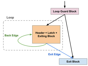
Figure 10.9 – Structure and terminology of a rotated loop
To get a rotated loop, you can run LoopRotationPass over the original loop. To check if a loop is rotated, you can use the Loop::isRotatedForm method.
This rotated form is basically transforming an arbitrary loop into a do{…}while(…) loop (in C/C++) with some extra checks. More specifically, let's say we have the following for loop:
// `N` is not a constant
for (int i = 0; i < N; ++i){…}
Loop rotation effectively turns it into the following code:
if (i < N) {
do {
…
++i;
} while(i < N);
}
The highlighted boundary check in the preceding code is used to ensure that the loop won't execute if the i variable is out of bounds at the very beginning. We also call this check the loop guard, as shown in the preceding diagram.
In addition to the loop guard, we also found that a rotated loop has a combined header, latch, and exiting block. The rationale behind this is to ensure that every instruction in this block has the same execution count. This is a useful property for compiler optimizations such as loop vectorization.
With that, we have learned about the various loop terminologies and the definition of canonical loops in LLVM. In the next section, we will learn about some APIs that can help you inspect some of these properties and process loops in an efficient way.
Learning about loop infrastructure in LLVM
In the Learning about loop representation in LLVM section, we learned about the high-level construction and important properties of a loop in LLVM IR. In this section, we are going to see what APIs are available for us to inspect those properties and further transform the loops. Let's start our discussion from the loop pass – the LLVM pass that applies to Loop instances.
In Chapter 9, Working with PassManager and AnalysisManager, we learned that there are different kinds of LLVM pass that work on different IR units – for instance, we have seen passes for Function and Module. These two kinds of passes have a similar function signature for their run method – the main entry point of an LLVM pass – as shown here:
PreservedAnalyses run(<IR unit class> &Unit,
<IR unit>AnalysisManager &AM);
Both of their run methods take two arguments – a reference to the IR unit instance and an AnalysisManager instance.
In contrast, a loop pass has a slightly more complicated run method signature, as shown here:
PreservedAnalyses run(Loop &LP, LoopAnalysisManager &LAM,
LoopStandardAnalysisResults &LAR,
LPMUpdater &U);
The run method takes four arguments, but we already know about the first two. Here are the descriptions for the other two:
- The third argument, LoopStandardAnalysisResults, provides you with some analysis data instances, such as AAResults (alias analysis data), DominatorTree, and LoopInfo. These analyses are extensively used by many loop optimizations. However, most of them are managed by either FunctionAnalysisManager or ModuleAnalysisManager. This means that, originally, developers needed to implement more complicated methods – for example, using the OuterAnalysisManagerProxy class – to retrieve them. The LoopStandardAnalysisResults instance basically helps you retrieve this analysis data ahead of time.
- The last argument is used for notifying PassManager of any newly added loops so that it can put those new loops into the queue before processing them later. It can also tell the PassManager to put the current loop into the queue again.
When we are writing a pass, we will want to use the analysis data provided by AnalysisManager – in this case, it is the LoopAnalysisManager instance. LoopAnalysisManager has a similar usage to other versions of AnalysisManager (FunctionAnalysisManager, for example) we learned about in the previous chapter. The only difference is that we need to supply an additional argument to the getResult method. Here is an example:
PreservedAnalyses run(Loop &LP, LoopAnalysisManager &LAM,
LoopStandardAnalysisResults &LAR,
LPMUpdater &U) {
…
LoopNest &LN = LAM.getResult<LoopNestAnalysis>(LP, LAR);
…
}
LoopNest is the analysis data that's generated by LoopNestAnalysis. (We will talk about both shortly in the Dealing with nested loops section.)
As shown in the previous snippet, LoopAnalysisManager::getResult takes another LoopStandarAnalysisResults type argument, in addition to the Loop instance.
Except for having different a run method signature and a slightly different usage of LoopAnalysisManager, developers can build their loop passes in the same way as other kinds of passes. Now that we've looked at the foundation provided by loop pass and AnalysisManager, it's time to look at some specialized loops. The first one we are going to introduce is the nested loop.
Dealing with nested loops
So far, we have been talking about loops with only one layer. However, nested loops – loops with other loop(s) enclosed in them – are also common in real-world scenarios. For example, most of the matrix multiplication implementations require at least two layers of loops.
Nested loops are usually depicted as a tree – called a loop tree. In a loop tree, every node represents a loop. If a node has a parent node, this means that the corresponding loop is enclosed within the loop being modeled by the parent. The following diagram shows an example of this:

Figure 10.10 – A loop tree example
In the preceding diagram, loops j and g are enclosed within loop i, so they are both child nodes of loop i in the loop tree. Similarly, loop k – the innermost loop – is modeled as the child node of loop j in the tree.
The root of a loop tree also represents a top-level loop in a Function. Recall that, previously, we learned how to retrieve all Loop instances in a Function by iterating through the LoopInfo object – each of the Loop instances that were retrieved in this way are top-level loops. For a given Loop instance, we can retrieve its subloops at the next layer in a similar way. Here is an example:
// `LP` has the type of `Loop&`
for (Loop *SubLP : LP) {
// `SubLP` is one of the sub-loops at the next layer
}
Note that the preceding snippet only traversed the subloops at the next level, rather than all the descendant subloops. To traverse all descendant subloops in a tree, you have two options:
- By using the Loop::getLoopsInPreorder() method, you can traverse all the descendant loops of a Loop instance in a pre-ordered fashion.
- In the Iterating different IR units section, we have learned what GraphTraits is and how LLVM uses it for graph traversal. It turns out that LLVM also has a default implementation of GraphTraits for the loop tree. Therefore, you can traverse a loop tree with existing graph iterators in LLVM, such as post-ordering and depth-first, to name a few. For example, the following code tries to traverse a loop tree rooted at RootL in a depth-first fashion:
#include "llvm/Analysis/LoopInfo.h"
#include "llvm/ADT/DepthFirstIterator.h"
…
// `RootL` has the type of `Loop*`
for (Loop *L : depth_first(RootL)) {
// Work with `L`
}
With the help of GraphTraits, we can have more flexibility when it comes to traversing a loop tree.
In addition to dealing with individual loops in a loop tree, LLVM also provides a wrapper class that represents the whole structure – LoopNest.
LoopNest is analysis data that's generated by LoopNestAnalysis. It encapsulates all the subloops in a given Loop instance and provides several "shortcut" APIs for commonly used functionalities. Here are some of the important ones:
- getOutermostLoop()/getInnermostLoop(): These utilities retrieve the outer/innermost Loop instances. These are pretty handy because many loop optimizations only apply to either the inner or outermost loop.
- areAllLoopsSimplifyForm()/areAllLoopsRotatedForm(): These useful utilities tell you if all the enclosing loops are in a certain canonical form, as we mentioned in the previous section.
- getPerfectLoops(…): You can use this to get all the perfect loops in the current loop hierarchy. By perfect loops, we are referring to loops that are nested together without a "gap" between them. Here is an example of perfect loops and non-perfect loops:
// Perfect loops
for(int i=…) {
for(int j=…){…}
}
// Non-perfect loops
for(int x=…) {
foo();
for(int y=…){…}
}
In the non-perfect loops example, the foo call site is the gap between the upper and lower loops.
Perfect loops are preferrable in many loop optimizations. For example, it's easier to unroll perfectly nested loops – ideally, we only need to duplicate the body of the innermost loop.
With that, you've learned how to work with nested loops. In the next section, we are going to learn about another important topic for loop optimization: induction variables.
Retrieving induction variables and their range
The induction variable is a variable that progresses by a certain pattern in each loop iteration. It is the key to many loop optimizations. For example, in order to vectorize a loop, we need to know how the induction variable is used by the array – the data we want to put in a vector – within the loop. The induction variable can also help us resolve the trip count – the total number of iterations – of a loop. Before we dive into the details, the following diagram shows some terminology related to induction variables and where they're located in the loop:

Figure 10.11 – Terminology for an induction variable
Now, let's introduce some APIs that can help you retrieve the components shown in the preceding diagram.
First, let's talk about the induction variable. The Loop class already provides two convenient methods for retrieving the induction variable: getCanonicalInductionVariable and getInductionVariable. Both methods return a PHINode instance as the induction variable (if there are any). The first method can only be used if the induction variable starts from zero and only increments by one on each iteration. On the other hand, the second method can handle more complicated cases, but requires a ScalarEvolution instance as the argument.
ScalarEvolution is an interesting and powerful framework in LLVM. Simply put, it tries to track how values change – for example, through arithmetic operation – over the program path. Putting this into the context of loop optimization, it is used to capture recurrence value-changing behaviors in the loop, which has a strong relationship with the induction variable.
To find out more about the induction variable's behavior in a loop, you can retrieve an InductionDescriptor instance via Loop::getInductionDescriptor. An InductionDescriptor instance provides information such as the initial value, the step value, and the instruction that updates the induction variable at each iteration. The Loop class also provides another similar data structure for realizing the boundaries of the induction variable: the Loop::LoopBounds class. LoopBounds not only provides the initial and step values of the induction variable, but also the prospective ending value, as well as the predicate that's used for checking the exit condition. You can retrieve a LoopBounds instance via the Loop::getBounds method.
Loops are crucial for a program's runtime performance. In this section, we learned how loops are represented in LLVM IR and how to work with them. We also looked at their high-level concepts and various practical APIs for retrieving the desired loop properties. With this knowledge, you are one step closer to creating a more effective, aggressive loop optimization and gaining even higher performance from your target applications.
Summary
In this section, we learned about LLVM IR – the target-independent intermediate representation that sits at the core of the entire LLVM framework. We provided an introduction to the high-level structure of LLVM IR, followed by practical guidelines on how to walk through different units within its hierarchy. We also focused on instructions, values, and SSA form at, which are crucial for working with LLVM IR efficiently. We also presented several practical skills, tips, and examples on the same topic. Last but not least, we learned how to process loops in LLVM IR – an important technique for optimizing performance-sensitive applications. With these abilities, you can perform a wider range of program analysis and code optimization tasks on LLVM IR.
In the next chapter, we will learn about a collection of LLVM utilities APIs that can improve your productivity when it comes to developing, diagnosing, and debugging with LLVM.