Chapter 4
Fully Connected Networks Applied to Multiclass Classification
In the first three chapters, we used our neural network to solve simple problems that set a foundation for learning deep learning (DL). We reviewed the basic workings of a neuron, how multiple neurons can be connected, and how to devise a suitable learning algorithm. Combining this knowledge, we built a network that can act as an XOR gate—something that arguably can be done in a simpler way.
In this chapter, we finally get to the point where we build a network that does something nontrivial. We show how to build a network that can take an image of a handwritten digit as input, identify which one of the ten digits 0 through 9 the image represents, and present this information on its outputs.
Before showing how to build such a network, we introduce some concepts that are central to both traditional machine learning (ML) and deep learning (DL), namely, datasets and generalization.
The programming example also provides more details on how to modify both the networks and the learning algorithm to handle the case of multiclass classification. This modification is needed because recognizing handwritten digits implies that each input example needs to be classified as belonging to one of ten classes.
Introduction to Datasets Used When Training Networks
As we saw in the previous chapters, we train a neural network by presenting an input example to the network. We then compare the network output to the expected output and use gradient descent to adjust the weights to try to make the network provide the correct output for a given input. A reasonable question is from where to get these training examples that are needed to train the network. For our previous toy examples this was not an issue. A two-input XOR gate has only four input combinations, so we could easily create a list of all combinations. This assumes that we interpret the input and output values as binary variables, which typically would not be the case but was true in our toy example.
In real applications of DL, obtaining these training examples can be a big challenge. One of the key reasons that DL has gained so much traction lately is that large online databases of images, videos, and natural language text have made it possible to obtain large sets of training data. If a supervised learning technique is used, it is not sufficient to obtain the input to the network. We also need to know the expected output, the ground truth, for each example. The process of associating each training input with an expected output is known as labeling, which is often a manual process. That is, a human must add a label to each example, detailing whether it is a dog, a cat, or a car. This process can be tedious because we often need many thousands of examples to achieve good results.
Starting to experiment with DL might be hard if the first step involved putting together a large collection of labeled training examples. Fortunately, other people have already done so and have made these examples publicly available. This is where the concept of datasets comes in. A (labeled) dataset consists of a collection of labeled training examples that can be used for training ML models. In this book, we will become familiar with a handful of different datasets within the fields of images, historical housing-price data, and natural languages. A section about datasets would not be complete without mentioning the classic Iris Dataset (Fisher, 1936), which is likely the first widely available dataset. It contains 150 instances of iris flowers, each instance belonging to one of three iris species. Each instance consists of four measurements (sepal length and width, petal length and width) of the particular plant. The Iris Dataset is extremely small and simple, so instead we start with a more complicated, although still simple, dataset: the Modified National Institute of Standards and Technology (MNIST) database of handwritten digits, also known simply as the MNIST dataset.
The MNIST dataset contains 60,000 training images and 10,000 test images. (We detail the differences between training and test images later in the chapter.) In addition to the images, the dataset consists of labels that describe which digit each image represents. The original images are 32×32 pixels, and the outermost two pixels around each image are blank, so the actual image content is found in the centered 28×28 pixels. In the version of the dataset that we use, the blank pixels have been stripped out, so each image is 28×28 pixels. Each pixel is represented by a grayscale value ranging from 0 to 255. The source of the handwritten digits is a mix of employees at the American Census Bureau and American high school students. The dataset was made available in 1998 (LeCun, Bottou, Bengio, et al., 1998). Some of the training examples are shown in Figure 4-1.
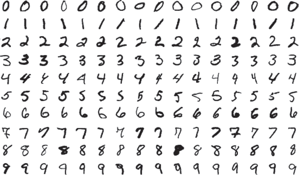
Figure 4-1 Images from the MNIST dataset. (Source: LeCun, Y., L. Bottou, Y. Bengio, and P. Haffner. “Gradient-Based Learning Applied to Document Recognition” in Proceedings of the IEEE vol. 86, no. 11 (Nov. 1998), pp. 2278–2324.)
Exploring the Dataset
We start with getting our hands dirty by exploring the dataset a little bit. First, you need to download it according to the instructions in Appendix I under “MNIST.” The file format is not a standard image format, but it is easy to read the files using the idx2numpy library.1 Code Snippet 4-1 shows how we load the files into NumPy arrays and then print the dimensions of these arrays.
1. Our understanding is that this library is not available on all platforms. Many online programming examples use a comma-separated value (CSV) version of the MNIST dataset instead. Consult the book’s website, http://www.ldlbook.com, for additional information.
Code Snippet 4-1 Load the MNIST Dataset and Inspect Its Dimensions
import idx2numpy
TRAIN_IMAGE_FILENAME = '../data/mnist/train-images-idx3-ubyte'
TRAIN_LABEL_FILENAME = '../data/mnist/train-labels-idx1-ubyte'
TEST_IMAGE_FILENAME = '../data/mnist/t10k-images-idx3-ubyte'
TEST_LABEL_FILENAME = '../data/mnist/t10k-labels-idx1-ubyte'

# Read files.
train_images = idx2numpy.convert_from_file(
    TRAIN_IMAGE_FILENAME)
train_labels = idx2numpy.convert_from_file(
    TRAIN_LABEL_FILENAME)
test_images = idx2numpy.convert_from_file(TEST_IMAGE_FILENAME)
test_labels = idx2numpy.convert_from_file(TEST_LABEL_FILENAME)

# Print dimensions.
print('dimensions of train_images: ', train_images.shape)
print('dimensions of train_labels: ', train_labels.shape)
print('dimensions of test_images: ', test_images.shape)
print('dimensions of test_images: ', test_labels.shape)
The output follows:
dimensions of train_images:  (60000, 28, 28)
dimensions of train_labels:  (60000,)
dimensions of test_images:  (10000, 28, 28)
dimensions of test_images:  (10000,)
The image arrays are 3D arrays where the first dimension selects one of the 60,000 training images or 10,000 test images. The other two dimensions represent the 28×28 pixel values (integers between 0 and 255). The label arrays are 1D arrays where each element corresponds to one of the 60,000 (or 10,000) images. Code Snippet 4-2 prints out the first training label and image pattern, and the resulting output follows.
Code Snippet 4-2 Print Out One Training Example
# Print one training example.
print('label for first training example: ', train_labels[0])
print('---beginning of pattern for first training example---')
for line in train_images[0]:
    for num in line:
        if num > 0:
            print('*', end = ' ')
        else:
            print(' ', end = ' ')
    print('')
print('---end of pattern for first training example---')
label for first training example:  5
---beginning of pattern for first training example---


                        * * * * * * * * * * * *
                * * * * * * * * * * * * * * * *
              * * * * * * * * * * * * * * * *
              * * * * * * * * * * *
                * * * * * * * * *
                  * * * * *
                      * * * *
                      * * * *
                        * * * * * *
                          * * * * * *
                            * * * * * *
                              * * * * *
                                  * * * *
                            * * * * * * *
                        * * * * * * * *
                    * * * * * * * * *
                * * * * * * * * * *
            * * * * * * * * * *
        * * * * * * * * * *
        * * * * * * * *


---end of pattern for first training example---
As shown from the example, it is straightforward to load and use this dataset.
Human Bias in Datasets
Because ML models learn from input data, they are susceptible to the garbage-in/garbage-out (GIGO) problem. It is therefore important to ensure that any used dataset is of high quality. A subtle problem to look out for is if the dataset suffers from human bias (or any other kind of bias). For example, a popular dataset available online is the CelebFaces Attributes (CelebA) dataset (Liu et al., 2015), which is derived from the CelebFaces dataset (Sun, Wang, and Tang, 2013). It consists of a large number of images of celebrities’ faces. Given how resource intensive it is to create a dataset, using a publicly available dataset makes sense. However, this dataset is biased in that it contains a larger proportion of white, young-looking individuals than is representative of society. This bias can have the effect that a model trained on this dataset does not work well for older or dark-skinned individuals.
Even if you have good intentions, you must actively consider the unintended consequences. A dataset that is influenced by structural racism in society can result in a model that discriminates against minorities.
To illustrate this point, it is worth noting that even a simple dataset like MNIST is susceptible to bias. The handwritten digits in MNIST originate from the American Census Bureau employees and American high school students. Not surprisingly, the digits will therefore be biased toward how people in the United States write digits. In reality, there are slight variations in the handwriting style across different geographical regions in the world. In particular, in some European and Latin American countries, it is common to add a second horizontal line when writing the digit 7. If you explore the MNIST dataset, you will see that although such examples are included, they are far from the majority of the examples of the digit 7 (only two of the 16 examples in Figure 4-1 have a second horizontal line). That is, as expected, the dataset is biased toward how people in the United States write these digits. Therefore, it may well be that a model trained on MNIST works better for people in the United States than for people from countries that use a different style for the digit 7.
Although this example likely is harmless in most cases, it serves as a reminder of how easy it is to overlook problems with the input data. Consider a self-driving car where the model needs to distinguish between a human being and a less vulnerable object. If the model has not been trained on a diverse dataset with enough representation of minority groups, then it can have fatal consequences.
Note that a good dataset does not necessarily reflect the real world. Using the self-driving car example, it is very important that the car can handle rare but dangerous events, such as an airplane emergency landing on the road. Therefore, a good dataset might well contain an overrepresentation of such events compared to what is present in the real world. This is somewhat different from human bias but is another example of how easy it is to make mistakes when selecting the dataset and how such mistakes can lead to serious consequences. Gebru and colleagues (2018) proposed datasheets for datasets to address this problem. Each released dataset should be accompanied by a datasheet that describes its recommended use and other details.
Training Set, Test Set, and Generalization
A reasonable question to ask is why we would go through the convoluted process of building a neural network to create a function that correctly predicts the output for a set of labeled examples. After all, it would be much simpler to just create a lookup table based on all the training examples. This brings us to the concept of generalization. The goal for an ML model is not just to provide correct predictions for data that it has been trained on; the more important goal is to provide correct predictions for previously unseen data. Therefore, we typically divide our dataset into a training dataset and a test dataset. The training dataset is used to train the model, and the test dataset is used to later evaluate how well the model was able to generalize to previously unseen data. If it turns out that the model does well on the training dataset but does poorly on the test dataset, then that is an indication that the model has failed to learn the general solution needed to solve similar but not identical examples. For example, it might have memorized only the specific training examples. To make this more concrete, consider the case of teaching children addition. You can tell them that 1 + 1 = 2 and 2 + 2 = 4 and 3 + 2 = 5, and they might later successfully repeat the answer when asked, What is 3 + 2? yet be unable to answer, What is 1 + 3? or even What is 2 + 3? (reversing the order of 3 and 2 compared to the training examples). This would indicate that the child has memorized the three examples but not understood the concept of addition.
We think that even somebody who knows addition and multiplication typically uses memorized answers for many small numbers and invoke generalized knowledge only for large numbers. On the other hand, we could argue that this is an example of deep learning whereby we hierarchically combine simpler representations into the final answer.
We can monitor the training error and test error during training to establish whether the model is learning to generalize; see Figure 4-2.
In general, the training error will show a downward trend until it finally flattens out. The test error, on the other hand, will often show a U-curve where it decreases in the beginning but then at some point starts increasing again. If it starts increasing while the training error is still decreasing, then that is a sign that the model is overfitting to the training data. That is, it learns a function that does really well on the training data but that is not useful on not-yet-seen data. Memorizing individual examples from the training set is one strong form of overfitting, but other forms of overfitting also exist. Overfitting is not the only reason for lack of generalization. It can also be that the training examples are simply not representative of the examples in the test set or, more important, the examples it will be used on in production.

Figure 4-2 How training error and test error can evolve during learning process
An effective technique to avoid overfitting is to increase the size of the training dataset, but there exist a number of other techniques, collectively known as regularization techniques, which are designed to reduce or avoid overfitting. One obvious method is early stopping. Simply monitor the test error during training and stop when it starts to increase. It is often the case that the error fluctuates during training and is not strictly moving in one direction or another, so it is not necessarily obvious when it is time to stop. One approach to determining when to stop is to save the weights of the model at fixed intervals during training (i.e., create checkpoints of the model along the way). At the end of training, identify the point with the lowest test error from a chart like the one in Figure 4-2, and reload the corresponding model.
The goal is for the network to learn to generalize. If the network does well on the training set but not on the test set, then that indicates overfitting to the training set. We increase the training dataset size or employ regularization techniques to avoid overfitting. One such technique is early stopping.
Hyperparameter Tuning and Test Set Information Leakage
It is extremely important to not leak information from the test set during the training process. Doing so can lead to the model memorizing the test set, and we end up with an overly optimistic assessment of how good our model is compared to how the model will perform in production. Information leakage can happen in subtle ways. When training a model, there is sometimes a need to tune various parameters that are not adjusted by the learning algorithm itself. These parameters are known as hyperparameters, and we have already encountered a few examples: learning rate, network topology (number of neurons per layer, number of layers, and how they are connected), and type of activation function. Hyperparameter tuning can be either a manual or an automated process. If we change these hyperparameters on the basis of how the model performs on the test set, then the test set risks influencing the training process. That is, we have introduced information leakage from the test set to the training process.
One way to avoid such leakage is to introduce an intermediate validation dataset. It is used for evaluating hyperparameter settings before doing a final evaluation on the test dataset. In our examples in this book, we keep it simple and only do manual tuning of hyperparameters, and we do not use a separate validation set. We recognize that by not using a validation set we run the risk of getting somewhat optimistic results. We discuss hyperparameter tuning and the validation dataset concept in more detail in Chapter 5, “Toward DL: Frameworks and Network Tweaks.”
Using a validation set for hyperparameter tuning is an important concept. See “Using a Validation Set to Avoid Overfitting,” in Chapter 5.
Training and Inference
Our experiments and discussion so far have focused on the process of training the network. We have interleaved testing of the network in the training process to assess how well the network is learning. The process of using the network without adjusting the weights is known as inference because the network is used to infer a result.
Training refers to coming up with the weights for the network and is typically done before deploying it into production. In production, the network is often used only for inference.
It is often the case that the training process is done only before the network is deployed in a production setting, and once the network is deployed, it is used only for inference. In such cases, training and inference may well be done on different hardware implementations. For instance, training might be done on servers in the cloud, and inference might be done on a less powerful device such as a phone or tablet.
Extending the Network and Learning Algorithm to Do Multiclass Classification
In the programming example in Chapter 3, our neural network had only a single output, and we saw how we could use that to identify a certain pattern. Now we want to extend our network to be able to indicate to which of ten possible classes a pattern belongs. One naïve way of doing that would be to simply create ten different networks. Each of them is responsible for identifying one specific digit type. It turns out that this is a somewhat inefficient approach. Regardless of what digit we want to classify, there are some commonalities among the different digits, so it is more efficient if each “digit identifier” shares many of the neurons. This strategy also forces the shared neurons to generalize better and can reduce the risk of overfitting.
One way of arranging a network to do multiclass classification is to create one output neuron per class and teach the network to output a one-hot encoded number. One-hot encoding implies that only one of the outputs is excited (hot) at any one point in time. One-hot encoding is an example of a sparse encoding, which means that most of the signals are 0. Readers familiar with binary numbers might find this inefficient and wonder if it would make more sense to use binary encoding, to reduce the number of output neurons, but that is not necessarily the most suitable encoding for a neural network.
Binary encoding is an example of a dense encoding, which means that we have a good mix of 1s and 0s. We discuss sparse and dense encodings further in Chapter 12, “Neural Language Models and Word Embeddings.” In Chapter 6, “Fully Connected Networks Applied to Regression,” we describe how to use a variation of one-hot encoding to make the network express various levels of certainty in its classification when it is unsure to which class an example belongs. For now, one-hot serves the purpose for the example we are interested in.
Network for Digit Classification
This section presents the network architecture we use in our handwritten digit classification experiment. This architecture is far from optimal for this task, but our goal is to quickly get our hands dirty and demonstrate some impressive results while still relying only on the concepts that we have learned so far. Later chapters explore more advanced networks for image classification.
As previously described, each image contains 784 (28×28) pixels, so our network needs to have 784 input nodes. These inputs are fed to a hidden layer, which we have arbitrarily chosen to have 25 neurons. The hidden layer feeds an output layer consisting of ten neurons, one for each digit that we want to recognize. We use tanh as an activation function for the hidden neurons and the logistic sigmoid function for the output layer. The network is fully connected; that is, each neuron in one layer connects to all neurons in the next layer. With only a single hidden layer, this network does not qualify as a deep network. At least two hidden layers are needed to call it DL, although that distinction is irrelevant in practice. The network is illustrated in Figure 4-3.

Figure 4-3 Network for digit classification. A large number of neurons and connections have been omitted from the figure to make it less cluttered. In reality, each neuron in a layer is connected to all the neurons in the next layer.
One thing that seems odd in Figure 4-3 is that we are not explicitly making use of information about how the pixels are spatially related to each other. Would it not be beneficial for a neuron to look at multiple neighboring pixels together? The way they are laid out in the figure as a 1D vector instead of a 2D grid, it appears that information related to which pixels are neighboring each other is lost. Two pixels neighboring each other in the y-direction are separated by 28 input neurons. This is not completely true. In a fully connected network, there is no such thing as pixels being “separated.” All 25 hidden neurons see all 784 pixels, so all pixels are equally close to each other from the perspective of a single neuron. We could just as well have arranged the pixels and neurons in a 2D grid, but it would not have changed the actual connections. However, it is true that we are not communicating any prior knowledge about which pixels are neighboring each other, so if it truly is beneficial to somehow take the spatial relationship between pixels into account, then the network will have to learn this by itself. In Chapter 7, “Convolutional Neural Networks Applied to Image Classification,” we learn about how to design networks in a way that does take the pixel location into account.
Loss Function for Multiclass Classification
When we solved the XOR problem, we used mean squared error (MSE) as our loss function. We can do the same in this image classification problem but must modify our approach slightly to account for our network having multiple outputs. We can do that by defining our loss (error) function as the sum of the squared error for each individual output:
where m is the number of training examples and n is the number of outputs. That is, in addition to the outer sum that computes the mean, we have now introduced an inner sum in the formula, which sums up the squared error for each output. To be perfectly clear, for a single training example, we end up with the following:
where n is the number of outputs and ŷj refers to the output value of neuron Yj. To simplify our derivative later, we can play the same trick as before and divide by 2 because minimizing a loss function that is scaled by 0.5 will result in the same optimization process as minimizing the unscaled loss function:
In this formula, we wrote the error function as a function of ŷ, which represents the output of the network. Note that ŷ is now a vector because the assumed network has multiple output neurons. Given this loss function, we can now compute the error term for each of the n output neurons, and once that is done, the backpropagation algorithm is no different from what we did in Chapter 3. The following formula shows the error term for neuron Y1 with output value ŷ1:
When computing the derivative of the loss function with respect to a specific output, all the other terms in the sum are constants (derivative is 0), which eliminates the sum altogether, and the error term for a particular neuron ended up being the same as in the single-output case. That is, the error term for neuron Y2 is –(y2 – ŷ2), or in the general case, the error term for Yj is –(yj – ŷj).
If these formulas seem confusing, take heart: Things become clear as we now dive into the programming example implementation and see how all of this works out in practice.
Programming Example: Classifying Handwritten Digits
As mentioned in the preface, this programming example is heavily influenced by Nielsen’s (2019) online book, but we have put our own personal touch on it to align with the organization of this book. Our implementation of the image classification experiment is a modified version of the implementation of the XOR learning example in Chapter 3, so the code should look familiar. One difference is that Code Snippet 4-3 contains some initializations where we now provide paths to the training and test datasets instead of defining the training values as hardcoded variables. We also tweaked the learning rate to 0.01 and introduced a parameter EPOCHS. We describe what an epoch is and discuss why we tweaked the learning rate later in the chapter. The dataset is assumed to be in the directory ../data/mnist/, as described in the dataset section of Appendix I.
Code Snippet 4-3 Initialization Section for MNIST Learning
import numpy as np
import matplotlib.pyplot as plt
import idx2numpy
np.random.seed(7) # To make repeatable
LEARNING_RATE = 0.01
EPOCHS = 20
TRAIN_IMAGE_FILENAME = '../data/mnist/train-images-idx3-ubyte'
TRAIN_LABEL_FILENAME = '../data/mnist/train-labels-idx1-ubyte'
TEST_IMAGE_FILENAME = '../data/mnist/t10k-images-idx3-ubyte'
TEST_LABEL_FILENAME = '../data/mnist/t10k-labels-idx1-ubyte'
We have also added a function to read the datasets from files, as shown in Code Snippet 4-4. A common theme in our coding examples is that there is some data preprocessing required, which can be somewhat tedious, but unfortunately, there is no good way around it.
Code Snippet 4-4 Read Training and Test Data from Files
# Function to read dataset.
def read_mnist():
    train_images = idx2numpy.convert_from_file(
        TRAIN_IMAGE_FILENAME)
    train_labels = idx2numpy.convert_from_file(
        TRAIN_LABEL_FILENAME)
    test_images = idx2numpy.convert_from_file(
        TEST_IMAGE_FILENAME)
    test_labels = idx2numpy.convert_from_file(
        TEST_LABEL_FILENAME)

    # Reformat and standardize.
    x_train = train_images.reshape(60000, 784)
    mean = np.mean(x_train)
    stddev = np.std(x_train)
    x_train = (x_train - mean) / stddev
    x_test = test_images.reshape(10000, 784)
    x_test = (x_test - mean) / stddev

    # One-hot encoded output.
    y_train = np.zeros((60000, 10))
    y_test = np.zeros((10000, 10))
    for i, y in enumerate(train_labels):
        y_train[i][y] = 1
    for i, y in enumerate(test_labels):
        y_test[i][y] = 1
    return x_train, y_train, x_test, y_test

# Read train and test examples.
x_train, y_train, x_test, y_test = read_mnist()
index_list = list(range(len(x_train))) # Used for random order
We already know the format of these files from the initial exercise where we explored the dataset. To simplify feeding the input data to the network, we reshape the images from two dimensions into a single dimension. That is, the arrays of images are now 2D instead of 3D. After this, we scale the pixel values and center them around 0. This is known as standardizing the data. In theory, this step should not be necessary because a neuron can take any numerical value as an input, but in practice, this scaling will be useful (we will explore why in Chapter 5). We first compute the mean and standard deviation of all the training values. We standardize the data by subtracting the mean from each pixel value and dividing by the standard deviation. This should be a familiar operation for anybody with a background in statistics. We do not go into the detail here but just mention what the overall idea is. By subtracting the mean from each pixel value, the new mean of all pixels will be 0. The standard deviation is a measure of how spread out the data is, and dividing by the standard deviation changes the range of the data values. This implies that if the data values were previously spread out (high and low values), then they will be closer to 0 after this operation. In our case, we started with pixel values between 0 and 255, and after standardization, we will end up with a set of floating-point numbers centered around and much closer to 0.
Knowing about data distributions and how to standardize them is an important topic, but we believe that you can make progress without understanding the details at this point.
Standard deviation is a measure of the spread of the data. A data point is standardized by subtracting the mean and dividing by the standard deviation.
One thing to note is that we are using the mean and standard deviation from the training data even when we standardize the test data. At first, this might look like a bug, but it is intentional. The thinking here is that we want to apply exactly the same transformation to the test data as we do to the training data. A natural question is whether it would be better to compute the overall average of both training and test data, but that should never be done because you then introduce the risk of leaking information from the test data into the training process.
You should apply exactly the same transformation to the test data as you apply to your training data. Further, never use the test data to come up with the transformation in the first place because that risks leaking information from the test data into the training process.
The next step is to one-hot encode the digit number to be used as a ground truth for our ten-output network. We one-hot encode by creating an array of ten numbers, each being 0 (using the NumPy zeros function), and then set one of them to 1.
Let us now move on to our implementation of the layer weights and the instantiation of our network in Code Snippet 4-5. This is similar to the XOR example, but there are a couple of changes. Each neuron in the hidden layer will have 784 inputs + bias, and each neuron in the output layer will have 25 inputs + bias. The for loop that initializes the weights starts with i=1 and therefore does not initialize the bias weight but just leaves it at 0 as before. The range for the weights is different than in our XOR example (magnitude of 0.1 instead of 1.0). We discuss that further in Chapter 5.
Code Snippet 4-5 Instantiation and Initialization of All Neurons in the System
def layer_w(neuron_count, input_count):
    weights = np.zeros((neuron_count, input_count+1))
    for i in range(neuron_count):
        for j in range(1, (input_count+1)):
            weights[i][j] = np.random.uniform(-0.1, 0.1)
    return weights

# Declare matrices and vectors representing the neurons.
hidden_layer_w = layer_w(25, 784)
hidden_layer_y = np.zeros(25)
hidden_layer_error = np.zeros(25)

output_layer_w = layer_w(10, 25)
output_layer_y = np.zeros(10)
output_layer_error = np.zeros(10)
Code Snippet 4-6 shows two functions that are used to report progress and to visualize the learning process. The function show_learning is called multiple times during training; it simply prints the current training and test accuracy and stores these values in two arrays. The function plot_learning is called at the end of the program and uses the two arrays to plot the training and test error (1.0 minus accuracy) over time.
Code Snippet 4-6 Functions to Report Progress on the Learning Process
chart_x = [] chart_y_train = [] chart_y_test = [] defshow_learning(epoch_no, train_acc, test_acc): global chart_x global chart_y_train global chart_y_test print('epoch no:', epoch_no, ', train_acc: ', '%6.4f' % train_acc, ', test_acc: ', '%6.4f' % test_acc) chart_x.append(epoch_no + 1) chart_y_train.append(1.0 - train_acc) chart_y_test.append(1.0 - test_acc) defplot_learning(): plt.plot(chart_x, chart_y_train, 'r-', label='training error') plt.plot(chart_x, chart_y_test, 'b-', label='test error') plt.axis([0, len(chart_x), 0.0, 1.0]) plt.xlabel('training epochs') plt.ylabel('error') plt.legend() plt.show()
Code Snippet 4-7 contains the functions for the forward and backward passes as well as for adjusting the weights. The forward_pass and backward_pass functions also implicitly define the topology of the network.
Code Snippet 4-7 Functions for Forward Pass, Backward Pass, and Weight Adjustment
defforward_pass(x): global hidden_layer_y global output_layer_y # Activation function for hidden layer for i, w in enumerate(hidden_layer_w): z = np.dot(w, x) hidden_layer_y[i] = np.tanh(z) hidden_output_array = np.concatenate( (np.array([1.0]), hidden_layer_y)) # Activation function for output layer for i, w in enumerate(output_layer_w): z = np.dot(w, hidden_output_array) output_layer_y[i] = 1.0 / (1.0 + np.exp(-z)) defbackward_pass(y_truth): global hidden_layer_error global output_layer_error # Backpropagate error for each output neuron # and create array of all output neuron errors. for i, y in enumerate(output_layer_y): error_prime = -(y_truth[i] - y) # Loss derivative derivative = y * (1.0 - y) # Logistic derivative output_layer_error[i] = error_prime * derivative for i, y in enumerate(hidden_layer_y): # Create array weights connecting the output of # hidden neuron i to neurons in the output layer. error_weights = [] for w in output_layer_w: error_weights.append(w[i+1]) error_weight_array = np.array(error_weights) # Backpropagate error for hidden neuron. derivative = 1.0 - y**2 # tanh derivative weighted_error = np.dot(error_weight_array, output_layer_error) hidden_layer_error[i] = weighted_error * derivative defadjust_weights(x): global output_layer_w global hidden_layer_w for i, error in enumerate(hidden_layer_error): hidden_layer_w[i] -= (x * LEARNING_RATE * error) # Update all weights hidden_output_array = np.concatenate( (np.array([1.0]), hidden_layer_y)) for i, error in enumerate(output_layer_error): output_layer_w[i] -= (hidden_output_array * LEARNING_RATE * error) # Update all weights
The forward_pass function contains two loops. The first one loops over all hidden neurons and presents the same input (the pixels) to them all. It also collects all the outputs of the hidden neurons into an array together with a bias term that can then be used as input to the neurons in the output layer. Similarly, the second loop presents this input to each of the output neurons and collects all the outputs of the output layer into an array that is returned to the caller of the function.
The backward_pass function is somewhat similar. It first loops through all the output neurons and computes the derivative of the loss function for each output neuron. In the same loop, it also computes the derivative of the activation function for each neuron. The error term for each neuron can now be calculated by multiplying the derivative of the loss function by the derivative of the activation function. The second loop in the function loops over all hidden neurons. For the hidden neurons, the error term is a little bit more complicated. It is computed as a weighted sum (computed as a dot product) of the backpropagated error from each of the output neurons, multiplied by the derivative of the activation function for the hidden neuron.
The adjust_weights function is straightforward, where we again loop over each neuron in each layer and adjust the weights using the input values and error terms.
Finally, Code Snippet 4-8 shows the network training loop. Instead of training until it gets everything correct, as we did in the XOR example, we now train for a fixed number of epochs. An epoch is defined as one iteration through all the training data. For each training example, we do a forward pass followed by a backward pass, and then we adjust the weights. We also track how many of the training examples were correctly predicted. We then loop through all the test examples and just record how many were correctly predicted. We use the NumPy argmax function to identify the array index corresponding to the greatest value; this decodes our one-hot encoded vector into an integer number. Before passing the input examples to forward_pass and adjust_weights, we extend each array with a leading 1.0 because these functions expect a bias term of 1.0 as the first entry in the array.
The NumPy function argmax() is a convenient way to find the element that the network predicts as being most probable.
We do not do any backward pass or weight adjustments for the test data. The reason for this is that we are not allowed to train on the test data because that will result in an optimistic assessment of how well the network works. At the end of each epoch, we print out the current accuracy for both the training data and the test data.
Code Snippet 4-8 Training Loop for MNIST
# Network training loop.
for i in range(EPOCHS): # Train EPOCHS iterations
    np.random.shuffle(index_list) # Randomize order
    correct_training_results = 0
    for j in index_list: # Train on all examples
        x = np.concatenate((np.array([1.0]), x_train[j]))
        forward_pass(x)
        if output_layer_y.argmax() == y_train[j].argmax():
            correct_training_results += 1
        backward_pass(y_train[j])
        adjust_weights(x)

    correct_test_results = 0
    for j in range(len(x_test)): # Evaluate network
        x = np.concatenate((np.array([1.0]), x_test[j]))
        forward_pass(x)
        if output_layer_y.argmax() == y_test[j].argmax():
            correct_test_results += 1
    # Show progress.
    show_learning(i, correct_training_results/len(x_train),
                  correct_test_results/len(x_test))
plot_learning() # Create plot
We run the program and get periodic progress printouts. Here are the first lines:
epoch no: 0 , train_acc:  0.8563 , test_acc:  0.9157
epoch no: 1 , train_acc:  0.9203 , test_acc:  0.9240
epoch no: 2 , train_acc:  0.9275 , test_acc:  0.9243
epoch no: 3 , train_acc:  0.9325 , test_acc:  0.9271
epoch no: 4 , train_acc:  0.9342 , test_acc:  0.9307
epoch no: 5 , train_acc:  0.9374 , test_acc:  0.9351
As before, your results might be slightly different due to random variations. When the program completes, it produces a chart, as shown in Figure 4-4. We see that both the training and the test error are decreasing over time, and the test error does not yet start to increase at the right side of a chart. That is, we do not seem to have a significant problem with overfitting. We do see that the training error is lower than the test error. This is common and not a reason for concern as long as the gap is not too big.

Figure 4-4 Training and test error when learning to classify digits
As shown from the progress printouts and the chart, the test error quickly falls below 10% (accuracy is above 90%); that is, our simple network can classify more than nine of ten images correctly. This is an amazing result given how simple the program is! Consider how lengthy a program you would need to write if you did not use an ML algorithm but instead tried to hardcode information about what defines the ten different digits. The beauty of ML is that instead of hardcoding this information yourself, the algorithm discovers this information from the training examples. In the case of a neural network, this information is encoded into the network weights.
We do not know how lengthy a program with a hardcoded approach would be, as we are lazy and have not bothered to try to write one. We just assume that it would be long because other people claim that this is the case.
Now sit back and relax for a moment, and think about what you have learned. You have gone from the description of the single neuron to connecting multiple neurons and applying a learning algorithm that results in a system that can classify handwritten digits!
The dataset used in this example was released in 1998. This was one year after Judgment Day in Terminator 2, when the war against the machines started and 3 billion human lives ended. That is, there is still some difference between fact and fiction.
Mini-Batch Gradient Descent
So far, we have been using stochastic gradient descent (SGD) as opposed to true gradient descent. As previously described, the distinction is that for SGD we compute the gradient for a single training example before updating the weights, whereas for true gradient descent, we would loop through the entire dataset and compute the average of the gradients for all training examples. There is a clear trade-off here. Looping through the entire dataset gives us a more accurate estimate of the gradient, but it requires many more computations before we update any weights. It turns out that a good happy medium is to use a small set of training examples known as a mini-batch. This enables more frequent weight updates (less computation per update) than true gradient descent while still getting a more accurate estimate of the gradient than when using just a single example. Further, modern hardware implementations, and in particular graphics processing units (GPUs), do a good job of computing a full mini-batch in parallel, so it does not take more time than computing just a single example.
The terminology is confusing here. The true gradient descent method uses batches (the entire training dataset) and is also known as batch gradient descent. At the same time, there is the hybrid between batch and stochastic gradient descent that uses mini-batches, but the size of a mini-batch is often referred to as batch size. Finally, SGD technically refers only to the case where a single training example is used (mini-batch size = 1) to estimate the gradient, but the hybrid approach with mini-batches is often also referred to as SGD. Thus, it is not uncommon to read statements such as “stochastic gradient descent with a mini-batch size of 64.” The mini-batch size is yet another parameter that can be tuned, and as of the writing of this book, anything close to the range of 32 to 256 makes sense to try. Finally, SGD (mini-batch size of 1, to be clear) is sometimes referred to as online learning because it can be used in an online setting where training examples are produced one by one instead of all being collected up front before learning begins.
From an implementation perspective, a mini-batch can be represented by a matrix because each individual training example is an array of inputs and an array of arrays becomes a matrix. Similarly, the weights for a single neuron can be arranged as an array, and we can arrange the weights for all neurons in a layer as a matrix. Computing the inputs to all activation functions for all neurons in the layer for all input examples in the mini-batch is then reduced to a single matrix-matrix multiplication. As previously mentioned, this is only a change in notation, but it does lead to significant performance improvements on platforms that have highly efficient matrix multiplication implementations. If you are interested, we have extended our plain Python implementation of our neural network to use matrices and mini-batches in Appendix F. It is perfectly fine to skip Appendix F, though, because these kinds of optimizations are already done (better) in the TensorFlow framework that is used in Chapter 5.
Concluding Remarks on Multiclass Classification
In this chapter, we implemented a network for handwritten digit classification. As opposed to the previous examples that all worked on binary classification, this was an example of a multiclass classification problem. The only real difference was to modify the network to have multiple output neurons and to define a suitable loss function. Apart from that, no new mechanisms were needed to train the network.
We should point out that the way we added multiple output neurons and the chosen loss function in this chapter are not the best-known solutions. We aimed for keeping things simple. In the next two chapters, we learn about better ways of doing this, namely, using the softmax output unit and the categorical cross-entropy loss function.
We also discussed the concept of dataset, a key part of enabling a model to learn. An important, and often overlooked, issue when selecting or creating a dataset is that it can pick up human biases, which may result in unintended consequences when using the trained model.
You are now well on your way toward exploring the field of DL. These first four chapters have been challenging because we introduced a lot of new concepts and implemented everything from scratch in Python. We believe that you will find the next couple of chapters easier when we introduce a DL framework that does much of the heavy lifting with respect to the low-level details. At the same time, you can feel comfortable knowing that there is no magic going on. The framework just provides efficient and easy-to-use implementations of the concepts that are described in this book.