Chapter 15
Attention and the Transformer
This chapter focuses on a technique known as attention. We start by describing the attention mechanism and how it can be used to improve the encoder-decoder-based neural machine translation architecture from Chapter 14, “Sequence-to-Sequence Networks and Natural Language Translation.” We then describe a mechanism known as self-attention and how the different attention mechanisms can be used to build an architecture known as the Transformer.
Many readers will find attention tricky on the first encounter. We encourage you to try to get through this chapter, but it is fine to skip over the details during the first reading. Focus on understanding the big picture. In particular, do not worry if you feel lost when you read about the Transformer architecture in the latter part of the chapter. Appendix D is the only part of the book that builds further upon this architecture. However, the Transformer is the basis for much of the significant progress made within natural language processing (NLP) in the last few years, so we encourage you to revisit the topic later if it is too heavy to get through the first time around.
Rationale Behind Attention
Attention is a general mechanism that can be applied to multiple problem domains. In this section, we describe how it can be used in neural machine translation. The idea with attention is that we let a network (or part of a network) decide for itself which part of the input data to focus on (pay attention to) during each timestep. The term input data in the previous sentence does not necessarily refer only to the input data to the overall model. It could be that parts of a network implement attention, in which case the attention mechanism can be used to decide what parts of an intermediate data representation to focus on. We soon give a more concrete example of what this means, but before doing so, let us briefly discuss the rationale behind this mechanism.
The attention mechanism can be applied to an encoder-decoder architecture and enables the decoder to selectively decide on which part of the intermediate state to focus.
Consider how a human translates a complicated sentence from one language to another, such as the following sentence from the Europarl dataset:
In my opinion, this second hypothesis would imply the failure of Parliament in its duty as a Parliament, as well as introducing an original thesis, an unknown method which consists of making political groups aware, in writing, of a speech concerning the Commission’s programme a week earlier—and not a day earlier, as had been agreed—bearing in mind that the legislative programme will be discussed in February, so we could forego the debate, since on the next day our citizens will hear about it in the press and on the Internet and Parliament will no longer have to worry about it.
We first read the sentence to get an overall idea of what it is trying to convey. We then start writing the translation, and while doing so, typically revisit different parts of the source sentence to ensure that our translation covers the entire sentence and describes it in an equivalent tense. The destination language might have a different preferred word order, such as in German where verbs appear as the last words in a sentence in past tense. Therefore, we might jump around in the source sentence to find a specific word when it is time for its translation to appear in the destination sentence. It seems reasonable to believe that a network would benefit from having that same flexibility.
Attention in Sequence-to-Sequence Networks
With that background, we now make the concept of attention more concrete by considering how a sequence-to-sequence-based neural machine translator (NMT) can be extended to include an attention mechanism. Let us start with a slightly different type of encoder-decoder network than we studied in Chapter 14. It is shown in Figure 15-1, and the difference is in how the encoder is connected to the decoder. In the previous chapter, the internal state from the last timestep of the encoding process was used as initial state at the first timestep for the decoder. In this alternative architecture, the internal state from the last timestep of the encoder is instead used as an input, accessible to the decoder at every timestep. The network also receives the embedding for the produced word from the last timestep as input. That is, the intermediate state from the encoder is concatenated with the embedding to form the overall input to the recurrent layer.
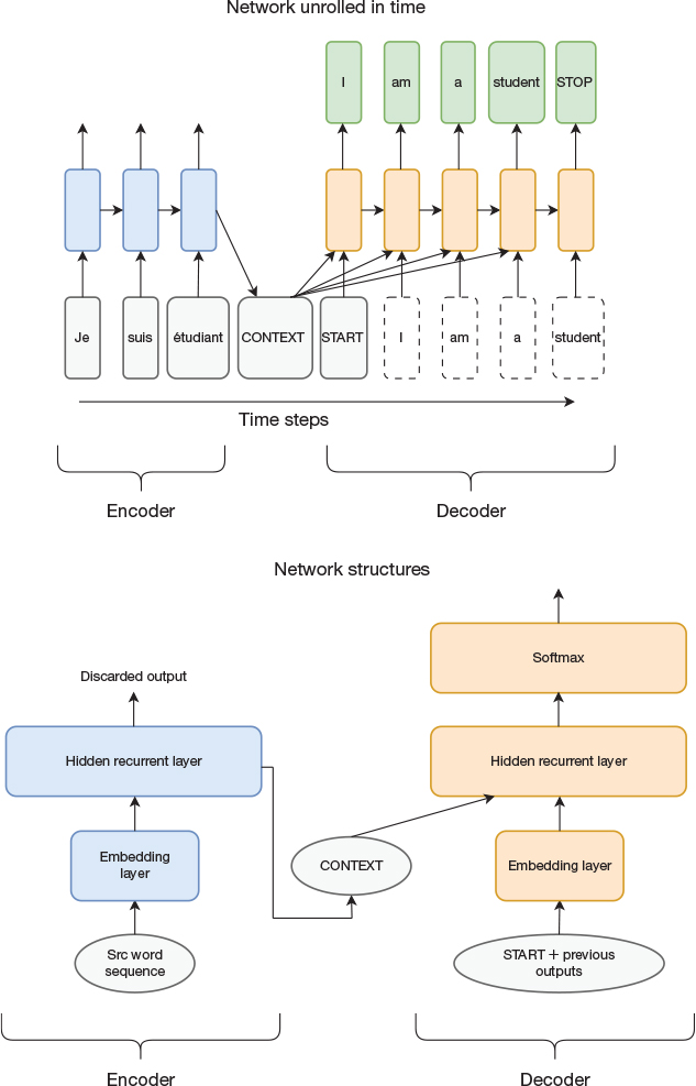
Figure 15-1 Alternative implementation of encoder-decoder architecture for neural machine translation. Top: Network unrolled in time. Bottom: The actual network structure (not unrolled).
This alternative sequence-to-sequence model can be found in a paper by Cho and colleagues (2014a), and we use it in this discussion simply because Bahdanau, Cho, and Bengio (2014) assumed that model as their baseline system when they added the attention mechanism to an NMT system. They observed that their model had a hard time dealing with long sentences and hypothesized that a reason was that the encoder was forced to encode the long sentence in a fixed-size vector. To resolve that problem, the authors modified their encoder architecture to instead read out the internal state at every timestep during the encoding process and store it for later access. This is illustrated in Figure 15-2. The top part of the figure shows the fixed-length encoding in a network without attention, using a vector length of 8. The bottom shows the attention case, where the encoding consists of one vector per input word.

Figure 15-2 Top: Fixed-length encoding in encoder-decoder network without attention. Bottom: Variable-length encoding in encoder-decoder network with attention.
An alternative way of connecting the encoder and decoder in a sequence-to-sequence network is to feed the encoder state as an input to the decoder for every timestep.
Although the figure shows it as one vector corresponding to each word, it is a little bit subtler than that. Each vector corresponds to the internal state of the decoder at the timestep for that word, but the encoding is influenced by both the current word and all historical words in the sentence.
The change to the encoder is trivial. Instead of discarding the internal state for all but the last timestep, we record the internal state for each timestep. This set of vectors is known as the source hidden state. It is also referred to as annotations or the more general term memory. We do not use those terms, but they are good to know when reading other publications on the topic.
The changes to the decoder are more involved. For each timestep, the attention-based decoder does the following:
1. Compute an alignment score for each state vector. This score determines how much attention to pay to that state vector during the current timestep. The details of the alignment score are described later in this chapter.
2. Use softmax to normalize the scores so they add up to 1. This vector of scores is known as the alignment vector and would consist of three values for the preceding example.
3. Multiply each state vector by its alignment score. Then add (elementwise) the resulting vectors together. This weighted sum (score is used as weight) results in a vector of the same dimension as in the network without attention. That is, in the example, it would be a single vector consisting of eight elements.
4. Use the resulting vector as an input to the decoder during this timestep. Just as in the network without attention, this vector is concatenated with the embedding from the previous timestep to form the overall input to the recurrent layer.
By examining the alignment scores for each timestep, it is possible to analyze how the model uses the attention mechanism during translation. This is illustrated in Figure 15-3. The three state vectors (one per encoder timestep) produced by the encoder are shown to the left. The four alignment vectors (one for each decoder timestep) are shown in the middle. For each decoder timestep, a decoder input is created by a weighted sum of the three encoder vectors. The scores in one of the alignment vectors are used as weights.

Figure 15-3 How encoder output state is combined with alignment vectors to create encoder input state for each timestep
For the preceding example, the decoder will keep its focus on je during the first timestep, which results in it outputting I. The color coding illustrates this (first decoder input is red, just like first encoder output). It will focus mainly on suis when outputting am. When outputting a, it focuses on both suis and étudiant (the input vector is green, which is a mix of blue and yellow). Finally, its focus is on étudiant when outputting student.
Bahdanau, Cho, and Bengio (2014) analyzed a more complex example:
French: L’ accord sur la zone économique européenne a été signé en août 1992.
English: The agreement on the European Economic Area was signed in August 1992.
Consider the words in bold. The word order is different in French than in English (zone corresponds to Area, and européenne corresponds to European). The authors show that for all three timesteps, when the decoder outputs European Economic Area, the alignment scores for all the three words zone économique européenne are high. That is, the decoder is paying attention to the neighboring words to arrive at a correct translation.
We now go through the attention mechanism for the decoder in more detail and, in particular, how to compute the alignment scores that result in this behavior. The architecture is outlined in Figure 15-4, where the upper part shows the workings of the network unrolled in time, with a focus on the second timestep for the decoder, and the lower part shows the network structures without unrolling.

Figure 15-4 Encoder-decoder architecture with attention
Starting with the unrolled view (top), we see that the intermediate representation consists of three pieces of state (one for each input timestep), each represented by a small white rectangle. As described previously in steps 2 and 3, we compute a weighted sum of these vectors to produce a single vector that is used as input to the recurrent layer in the decoder. The weights (also known as alignment scores or alignment vector) are adjustable and recomputed at each timestep. As you can see from the figure, the weights are controlled by the internal state of the decoder from the timestep before the current decoder timestep. That is, the decoder is responsible for computing the alignment scores.
The lower part of the figure shows a structural (not unrolled) view of the same network, where again it is apparent that, by adjusting the weights properly, the decoder itself controls how much of each encoder state vector to use as its input.
Computing the Alignment Vector
We now describe how to compute the alignment vector for each decoder timestep. An alignment vector consists of Te elements, where Te is the number of timesteps for the encoder. We need to compute Td such vectors, where Td is the number of timesteps for the decoder.
One can envision multiple ways of computing the alignment vector. We know that it needs to be of length Te. We also need to decide what input values to use to compute the vector. Finally, we need to decide what computation to apply to these input values to produce the scores.
One obvious candidate for input value is the decoder state because we want the decoder to dynamically be able to choose what parts of the input to focus on. We have already made this assumption in the high-level figures where the state outputs from the top recurrent layer in the decoder are used to control the weights in the attention mechanism (the weights in the high-level figures represent the alignment vector in the more detailed attention mechanism description). Another candidate that can be used as input values for this computation is the source hidden state. At first, this might seem a little bit hard to wrap your head around in that we will use the source hidden state to compute the alignment vector, which will then be used to determine what parts of the source hidden state will be visible to the decoder. However, this is not as strange as it seems. If you view the source hidden state as a memory, this means that we use the content of that memory to address what piece of the memory to read, a concept known as content addressable memory (CAM). We mention this for readers who already are familiar with CAM, but knowing details about CAM is not required to follow our remaining description of how to compute the alignment vector.
From a terminology perspective, in our example, the decoder state is used as a query. It is then used to match against a key, which in our case is the source hidden state. This selects the value to return, which in our case is also the source hidden state, but in other implementations, the key and value can be different from each other.
Now we just need to decide on the function that is used to match the query to the key. Given the topic of this book, it is not farfetched to use a neural network for this function and let the model learn the function itself. Figure 15-5 shows two potential implementations.
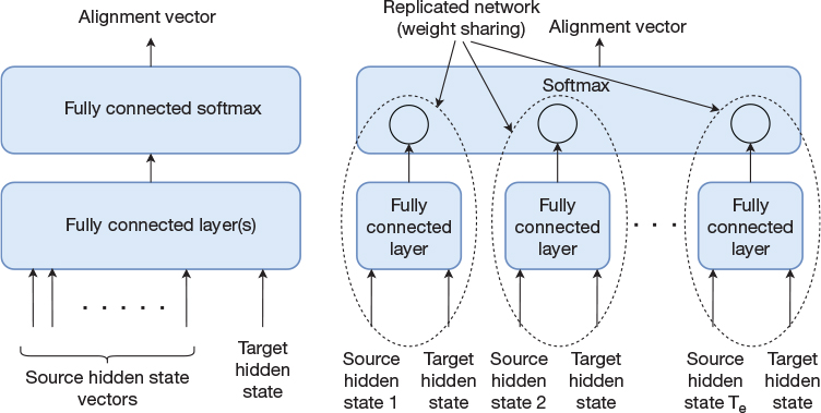
Figure 15-5 Two alternative implementations of the function that computes the alignment vector
The left part of the figure shows a fully connected feedforward network with an arbitrary number of layers, ending with a fully connected softmax layer that outputs the alignment vector. The softmax layer ensures that the sum of the elements in the alignment vector is 1.0. One drawback with the network in the left part of the figure is that we introduce restrictions on the source input length. More serious is that the leftmost network hardcodes the expected position of words in the source sentence, which can make it harder for the network to generalize. The rightmost architecture addresses this issue by having multiple instances of a two-layer network with weight sharing between the instances. As we have seen previously, weight sharing results in enabling the network to identify a specific pattern regardless of its position. Each instance of this fully connected network takes the target hidden state and one timestep of the source hidden state as inputs. The activation function for the first layer is tanh, and we use softmax in the output layer to ensure that the sum of the elements in the alignment vector results in 1.0. This architecture reflects the attention mechanism introduced by Bahdanau, Cho, and Bengio (2014).
Mathematical Notation and Variations on the Alignment Vector
Publications about attention mechanisms generally describe the attention function using linear algebra instead of drawing out networks as we have done. In this section, we first map the description and Figure 15-5 to mathematical equations. Once that is done, we present simplifications of the attention function, which can be done compactly using these equations.
The network starts with Te instances of a two-level network, where Te represents the number of encoder timesteps. The first layer uses tanh as an activation function. The second layer of each two-level network is a single neuron without an activation function (softmax is applied later). What we just described is represented by the networks in the dashed ovals in the figure, where the content of each oval implements a function known as a scoring function:
The target hidden state and one of the source hidden states are used as inputs to this scoring function. These two vectors are concatenated and multiplied by a matrix Wa after which the tanh function is applied. These operations correspond to the first fully connected layer. The resulting vector is then multiplied by a transposed version of vector va. This corresponds to the single neuron in the output layer in the dashed oval. We compute this scoring function for each encoder timestep. Each timestep results in a single value so, all in all, we get a vector with Te elements. We apply the softmax function to this vector to scale the values so the elements sum to 1. Each element of the output of the softmax operation is computed using the following formula:
In the formula, Te represents the number of encoder timesteps, and i is the index of the element that is computed. We organize the resulting elements into an alignment vector with one element for each encoder timestep:
There is nothing magical about the chosen scoring function. Bahdanau, Cho, and Bengio (2014) simply chose a two-level fully connected neural network to make it sufficiently complex to be able to learn a meaningful function yet simple enough to not be too computationally expensive. Luong, Pham, and Manning (2015) experimented with simplifying this scoring function and showed that the two simpler functions in Equation 15-1 also work well:
Equation 15-1 Simplifications of the scoring function
One natural question is what the two functions in Equation 15-1 represent in terms of neural networks. Starting with the dot product version, combined with the softmax function, this represents the network in the right part of Figure 15-5 but with the modification that there is no fully connected layer before the softmax layer. Further, the neurons in the softmax layer use the target hidden state vector as neuron weights, and the source hidden state vector are used as inputs to the network. The general version combined with the softmax function represents a first layer defined by Wa and with a linear activation function again followed by a softmax layer that uses the target hidden state vector as neuron weights. In reality, once we have started to think about these networks in terms of mathematical equations, we do not necessarily care about what a slight modification of an equation implies in terms of the network structure as long as it works well. Flipping things around, we can also analyze the mathematical equations to see if they can provide any insight into how the attention mechanism works. Looking at the dot product version, we know that the dot product of two vectors tends to be large if elements located in the same position in both vectors are of the same sign. Alternatively, consider the case where the vectors are produced by rectified linear units (ReLU) so that all elements are greater than or equal to zero. Then the dot product will be large if the vectors are similar to each other, in the sense that nonzero elements in both vectors are aligned with each other. In other words, the attention mechanism will tend to focus on timesteps where the encoder state is similar to the current decoder state. We can envision that this makes sense if the hidden states of the encoder and decoder somehow express the type of word that is currently being processed, such as if the current state can be used to determine whether the current word is the subject or the object in the sentence.
Attention in a Deeper Network
This description assumes a network with a single recurrent layer. Figure 15-6 shows a network architecture introduced by Luong, Pham, and Manning (2015) that applies attention to a deeper network. There are a couple of key differences compared to Figure 15-4. First, this network architecture is more similar to our original NMT in that we use the final encoder internal state to initialize the decoder internal state. Second, as opposed to Figure 15-4, we see that the encoder and decoder now have two or more recurrent layers. Luong, Pham, and Manning handled this by applying the attention mechanism only to the internal state of the topmost layer. Further, instead of using the context derived by the attention mechanism as input to a recurrent layer, this state is concatenated with the output of the top recurrent layer in the decoder and fed into a fully connected layer. The output of this fully connected layer is referred to as an attentional vector. This vector is fed back to the input of the first recurrent layer in the next timestep. In some sense, this makes the fully connected layer act as a recurrent layer as well and is key to making the attention mechanism work well. It enables the network to take into account what parts of the source sentence it has already attended to when deciding what parts of the source sentence to consider next. In the architecture in Figure 15-4, this explicit feedback loop was not needed because there is an implicit feedback loop given that the weighted state is fed to a recurrent layer instead of to a regular feedforward layer.

Figure 15-6 Alternative attention-based encoder-decoder architecture
A final key difference is that in Figure 15-6 the weighted sum is fed to a higher layer in the network instead of being fed back to the same layer that creates the state that controls the weights. This has the effect that the adjustable weights are now controlled by the state in the current decoder timestep instead of in the previous timestep. This might not be obvious at first when looking at the figure. When you consider how the data flows, you can see that in Figure 15-6 it is possible to compute the adjustable weights before using them, whereas in the Figure 15-4 the output of the adjustable weights is used to compute the vector that controls them. Hence, the vector that controls the weights must have been derived from a previous timestep.
Additional Considerations
In the attention mechanism we have described, the decoder creates a weighted sum of the vectors in the source hidden state. This is known as soft attention. An alternative is to instead let the decoder attend to only one out of the vectors in the source hidden state for each timestep. This is known as hard attention.
A benefit of computing a weighted sum is that the attention function is continuous and thereby differentiable. This enables the use of backpropagation for learning as opposed to when a discrete selection function is used.
In hard attention, the state from a single encoder timestep is selected to focus on each decoder timestep. In soft attention, a mixture (weighted sum) of the state from all encoder timesteps is used.
Finally, let us reflect on one of the restrictions that we now have applied to our sequence-to-sequence network. Before applying attention, the network could in theory accept an input sequence of unlimited length. However, the need for the attention mechanism to store the entire source hidden state, which grows linearly with the source sequence length, implies that we now have a limitation on the length of the input sequence. This might seem unfortunate at first, but it is of limited practical importance. Consider the fairly complex sentence that we gave as a rationale for the attention mechanism some paragraphs back. Few people would be able to read it once and then produce a good translation. In other words, the human brain has a hard time even remembering a sentence of such length and needs to rely on external storage (the paper or computer screen on which it is written) to create a good translation. In reality, the amount of storage needed to memorize the sentence is only 589 bytes in uncompressed form. With that background, having to reserve enough storage to keep track of the source hidden state seems reasonable.
This concludes our detailed description of the basic attention mechanism. One takeaway from this discussion is that attention is a general concept, and there are multiple potential ways to implement it. This may make you feel somewhat uneasy at first, in that it seems unclear that either one of the described implementations is the “right” way to do it. This reaction is similar to when first encountering the LSTM unit and the gated recurrent unit (GRU). In reality, there probably is not a single right way of applying these concepts. Different implementations express slightly different behavior and come with different efficiency levels in terms of how much computation is required to achieve a certain result.
Alternatives to Recurrent Networks
If we take a step back, a reasonable question is why we think that recurrent networks are required for our NMT. The starting point was that we wanted the ability to process variable sequence lengths for both the source and the destination sequences. The RNN-based encoder-decoder network was an elegant solution to this with a fixed-sized intermediate representation. However, to get good translations of long sentences, we then reintroduced some restrictions on the input sequence length and had the decoder access this intermediate state in a random-access fashion using attention. With that background, it is natural to explore whether we need an RNN to build our encoder or whether other network architectures are just as good or better. Another issue with the RNN-based implementation is that RNNs are inherently serial in nature. The computations cannot be parallelized as well as they can in other network architectures, leading to long training times. Kalchbrenner and colleagues (2016) and Gehring and colleagues (2017) studied alternative approaches that are based on convolutional networks with attention instead of recurrent networks.
A major breakthrough came with the introduction of the Transformer architecture (Vaswani et al., 2017). It uses neither recurrent layers nor convolutional layers. Instead, it is based on fully connected layers and two concepts known as self-attention (Lin, Doll, et al., 2017) and multi-head attention. A key benefit of the Transformer architecture is that it is parallel in nature. The computations for all input symbols (e.g., words in language translation) can be done in parallel with each other.
The Transformer is based on self-attention and multi-head attention.
The Transformer architecture has driven much of the progress in NLP since 2017. It has achieved record scores in language translation. It is also the basis for other important models. Two such models are Generative Pre-Training (GPT) and Bidirectional Encoder Representations from Transformers (BERT), which have achieved record scores on tasks within multiple NLP applications (Devlin et al., 2018; Radford et al., 2018). More details about GPT and BERT can be found in Appendix D.
GPT and BERT are language models based on the Transformer architecture.
The next couple of sections describe the details of self-attention and multi-head attention. We then move on to describe the overall Transformer architecture and how it can be used to build an encoder-decoder network for natural language translation without recurrent layers.
Self-Attention
In the attention mechanism we have studied so far, the decoder uses attention to direct focus to different parts of the intermediate state. Self-attention is different in that it is used to decide which part of the output from the preceding layer to focus on. This is shown in Figure 15-7, where self-attention is applied to the output of an embedding layer and is followed by a fully connected layer for each word. For each of these fully connected layers, the input will be a combination of all the words in the sentence, where the attention mechanism determines how heavily to weigh each individual word.
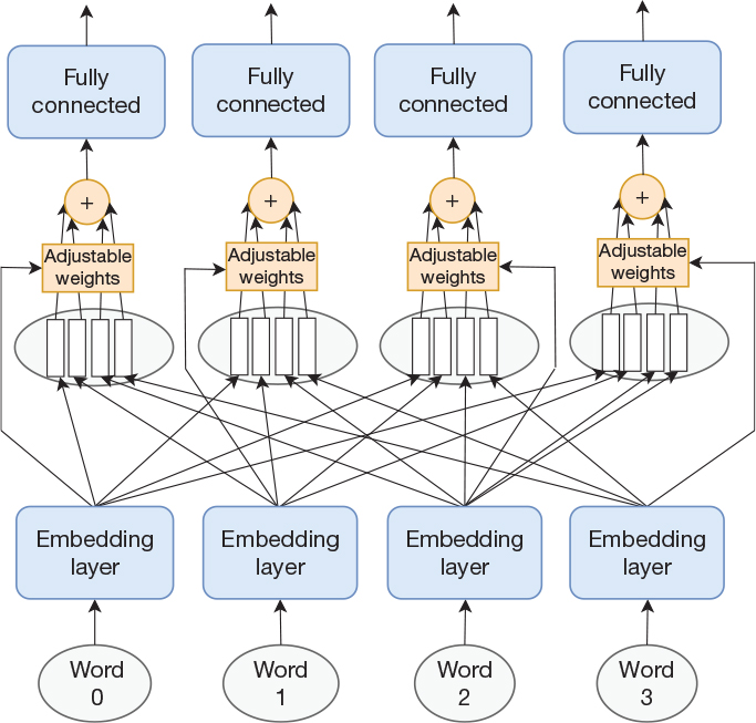
Figure 15-7 Embedding layer followed by a self-attention layer followed by a fully connected layer. The network employs weight sharing, so each word position uses the same weights.
Before diving into the details of the self-attention mechanism, it is worth pointing out how the architecture in the figure exposes parallelism. Although the figure contains multiple instances of embedding layers, attention mechanisms, and fully connected layers, they are all identical (weight sharing). Further, within a single layer, there are no dependencies between words. This enables an implementation to do the computations in parallel. Consider the inputs to the fully connected layers. We can arrange the four output vectors from the attention mechanisms into a matrix with four rows. The fully connected layer is represented by a matrix with one column per neuron. We can now compute the output for all four instances in parallel by a single matrix-matrix multiplication. We will see later how the self-attention mechanism exposes additional parallelism, but first we need to describe self-attention in more detail.
Earlier in this chapter, we described how the attention mechanism uses a scoring function to compute these weights. One of the inputs to this scoring function, the key, was the data value itself. The other input, the query (the horizontal arrows in Figure 15-7), came from the network that would consume the input (the decoder network). In the case of self-attention, the query comes from the previous layer, just as the value does.
The self-attention mechanism in the Transformer is slightly more complex than what is shown in the figure. Instead of directly using the inputs to the attention mechanism as key, query, and data, these three vectors are computed by three separate single-layer networks with linear activation functions. That is, the key is now different than the data value, and another side effect is that we can use a different width of key, query, and data than the original input. This is shown in Figure 15-8 for a single attention mechanism.
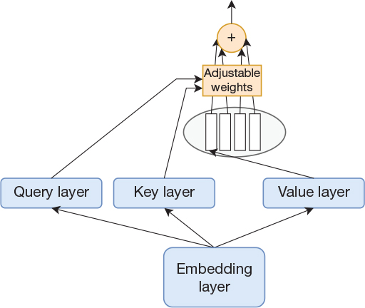
Figure 15-8 Attention mechanism with projection layers that modify the dimensions of the query, key, and value
It might seem confusing that we now have two arrows feeding into the rectangle with the adjustable weights. In the previous figures, we implicitly used the data values (the white rectangles) as both value and key, so we did not explicitly draw this arrow. That is, in reality, the attention mechanism did not change much despite the figure containing an additional arrow.
Multi-head Attention
We saw in the previous section how we can use self-attention to produce N output vectors from N input vectors, where N was the number of words that were input to the network. The self-attention mechanism ensured that all N input vectors could influence each output vector. We also introduced layers for the query, key, and value that enabled us to make the width of the output vector independent of the width of the input vector. The ability to decouple the input width from the output width is central in the multi-head attention concept.
Multi-head attention is as simple as having multiple attention mechanisms operating in parallel for each input vector. This is shown in Figure 15-9 for an example with two heads.
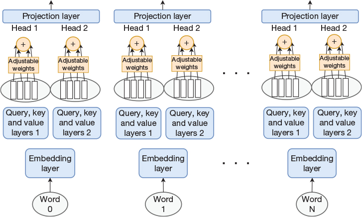
Figure 15-9 Embedding layer followed by multi-head self-attention layer. Each input word vector is processed by multiple heads. The output of all heads for a given word are then concatenated and run through a projection layer.
This figure implies that each input vector now results in two output vectors. That is, if the output width of a single head is the same as the input width, the output of the layer now has two times as many values as compared to the input to the layer. However, given the query, key, and value layers, we have the ability to size the output to any width. In addition, we have added a projection layer on the output. Its input is the concatenated output from the heads. All in all, this means that we have full flexibility in selecting the width of the attention heads as well as the overall output of the multi-head self-attention layer.
Just as for Figure 15-7, we assume weight sharing in Figure 15-9. The query layer for head 1 for word 0 is identical to the query layer for head 1 for all other words, and the same applies to the key and value layers. From an implementation perspective, this means that if we arrange our N input vectors to the self-attention layer into a matrix, computing the query vector for head 1 for all input vectors is equivalent to a single matrix-matrix multiplication. The same holds true for the key vector and the value vector. The number of heads is another level of parallelism, so in the end, the self-attention layer results in a large number of matrix multiplications that can be done in parallel.
The Transformer
As previously mentioned, the Transformer is an encoder-decoder architecture similar to what we have seen already, but it does not employ recurrent layers. We first describe the encoder, which starts with an embedding layer for each word, as we have seen in previous figures. The embedding layers are followed by a stack of six identical modules, where each module consists of a multi-head self-attention layer and a fully connected layer corresponding to each input word. In addition, each module employs skip connections and normalization, as shown in the left part of Figure 15-10, which illustrates a single instance of the six modules.
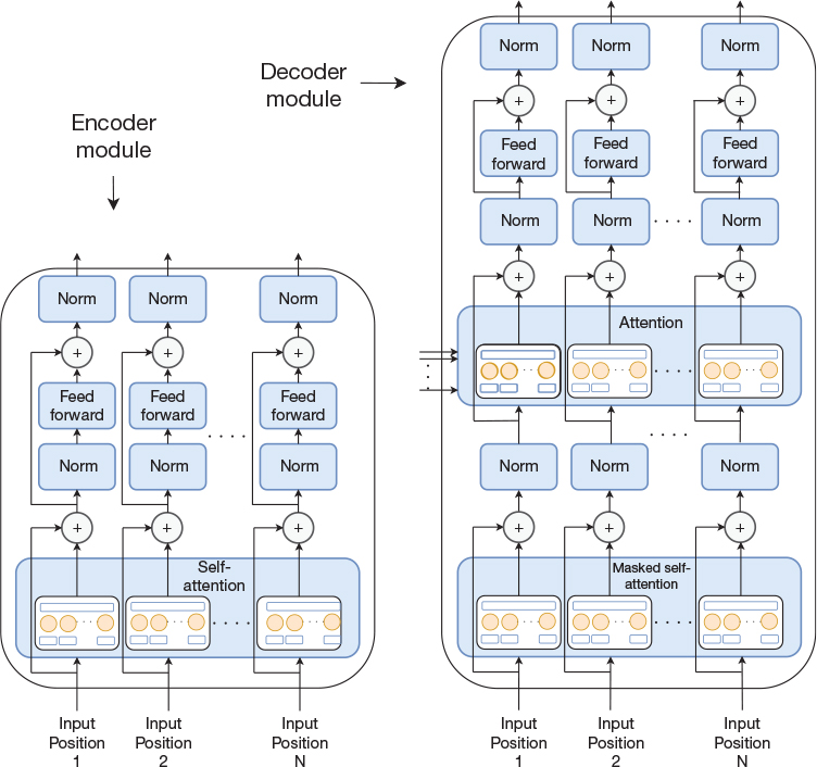
Figure 15-10 Left: Transformer encoder module consisting of multi-head self-attention, normalization, feedforward, and skip connections. The feedforward module consists of two layers. Right: Transformer decoder module. Similar to the encoder module but extended with a multi-head attention (not self-attention) in addition to the multi-head self-attention layer. The overall Transformer architecture consists of multiple encoder and decoder modules.
The network uses layer normalization (Ba, Kiros, and Hinton, 2016) as opposed to batch normalization that we have seen previously. Layer normalization has been shown to facilitate training just like batch normalization but is independent of the mini-batch size.
We stated that the Transformer does not use recurrent layers, but the decoder is still an autoregressive model. That is, it does generate the output one word at a time and still needs to feed each generated word back as an input to the decoder network in a serial fashion. Just as for the encoder, the decoder consists of six instances of a module, but this decoder module is slightly more complex than the encoder module. In particular, the multi-head self-attention mechanism includes a masking mechanism that prevents it from attending to future words, as they have not yet been generated. In addition, the decoder module contains another attention layer, which attends to the output from the encoder modules. That is, the decoder employs both self-attention and traditional attention to the intermediate state generated by the encoder. However, as opposed to our examples earlier in this chapter, in addition to using multi-head attention in the self-attention layers, the Transformer also uses multi-head attention in the attention layer that is applied to the intermediate state from the encoder. The decoder module is illustrated to the right in Figure 15-10.
Now that we have described the encoder module and the decoder module, we are ready to present the complete Transformer architecture. It is shown in Figure 15-11. The figure shows how the decoder attends to intermediate state produced by the encoder.
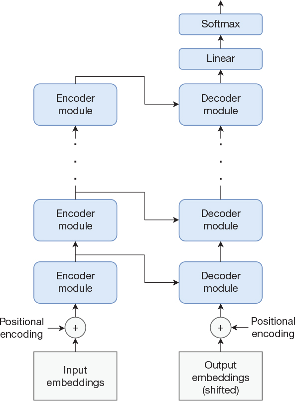
Figure 15-11 The transformer architecture
The figure contains one final detail that we have not yet described. If you consider how the overall Transformer architecture is laid out, it has no good way of taking word order into account. The words are not presented sequentially, as in a recurrent network, and the subnetworks that process each individual word all share weights. To address this issue, the Transformer architecture adds something called a positional encoding to each input embedding vector. The positional encoding is a vector with the same number of elements as the word embedding itself. This positional encoding vector is added (elementwise) to the word embedding, and the network can make use of it to infer the spatial relationship between words in the input sentence. This is illustrated in Figure 15-12, which shows an input sentence consisting of n words, where each word is represented by a word embedding with four elements.

Figure 15-12 Positional encodings are added to input embeddings to indicate word order. The figure assumes word embeddings with four elements. The sentence consists of n words. A positional encoding vector is added to the input embedding for each word to compute the resulting embedding that is fed to the network.
We need to compute one positional encoding vector corresponding to each input word. Clearly, the elements in the positional encoding vector should be influenced by the word’s position in the sentence. It also turns out to be beneficial if all elements in the positional encoding vector are not identical. That is, for a specific input word, we do not add the same value to each element in the word vector, but the value depends on the index in the word vector. The figure illustrates this by using different colors for the four elements in the positional encoding vector. If the index i of the element in the vector is even, the value of the element in the positional encoding vector is1
1. If you read the original paper (Vaswani et al., 2017), you will find that the equations are stated somewhat differently using 2i rather than i. This is not a typo. It results from the paper not using i to represent the index in the vector. Instead, it denotes the index by 2i for even indices and 2i+1 for odd indices.
where pos is the position of the word in the sentence, i is the index of the element in the vector, and d is the number of elements in the word embedding. If the index i of the element in the vector is odd, the value of the element is
From the formulas, we can see that for a given index i, the arguments to sin and cos are monotonically increasing from zero and upward as we move to later words in the sentence. It may not seem obvious why these positional encodings are the right ones to use. As with many other mechanisms, this is just one of many options. Architectures in Appendix D use another option, namely, to learn positional encodings during training.
Concluding Remarks on the Transformer
When the Transformer model was introduced, it produced better English-to-German and English-to-French translations than any previous models. Note that a Transformer-based translation network is still an example of an encoder-decoder architecture, just like the LSTM-based network in Chapter 14. However, the parallel nature of the encoder and decoder addresses the serialization problem presented by LSTM-based architectures.
The Transformer is useful not only for language translation tasks but also for NLP in general. As an example, in the programming example in Chapter 12, “Neural Language Models and Word Embeddings,” we implemented an LSTM-based language model. In contrast, the more recently published language models are based on components from the Transformer architecture. As we pointed out in Chapter 14, the decoder part of a translation network is basically a language model, which is initialized with the internal state of the encoder. A modified version of the Transformer decoder is used to implement the popular language model GPT, which is described in Appendix D. Another example, also described in Appendix D, is BERT, which is based on the encoder component from the Transformer architecture.
Earlier in this chapter, we stated that the Transformer uses neither recurrent layers nor convolutional layers. However, we also noted that the decoder component of the network is an autoregressive model and thereby does employ a feedback mechanism similar to recurrence. To be fair, this is more related to how the model is used and is not inherent in the model architecture. In fact, the BERT model is based solely on the Transformer encoder and is thereby completely free from such feedback connections. On the topic of convolutional layers, we note that although the Transformer does not explicitly use convolutions, it does make use of weight sharing similar to what convolutions do. Cordonnier, Loukas, and Jaggi (2020) studied how self-attention and convolutional layers relate to each other and showed that attention layers often learn to perform convolutions in practice. However, a key difference between self-attention and convolution is that the self-attention layer can attend to any position in the input, whereas convolutions can attend only to neighboring positions covered by the convolutional kernel.
To learn more about the Transformer, apart from reading the original paper, we recommend Alammar’s blog post about the Transformer (Alammar, 2018b). It also contains links to publicly available source code so you can get started with using the model. If you want to learn about more use cases of the Transformer architecture, consider reading about GPT, BERT, and RoBERTa in Appendix D now. Another option is to continue to Chapter 16, “One-to-Many Network for Image Captioning,” which describes how to build an attention-based model for image captioning.