Chapter 13
Word Embeddings from word2vec and GloVe
As previously mentioned, the evolution of neural language models and word embeddings are somewhat intertwined. Bengio and colleagues (2003) decided to use word embeddings in their neural language model, reasoning that it would help the language model to be effective. Collobert and Weston (2008) and Mikolov, Yih, and Zweig (2013) then discovered that the resulting word embeddings demonstrated noteworthy properties, which was also demonstrated by the programming example in Chapter 12, “Neural Language Models and Word Embeddings.” Mikolov, Chen, and colleagues (2013) explored whether word embeddings could be improved by making the properties of the embeddings the primary objective as opposed to just producing them as a byproduct in the process of trying to create a good language model. Their work resulted in the word2vec algorithm, which comes with a number of variations and is described in detail in this chapter.
Pennington, Socher, and Manning (2014) later devised a different algorithm, known as GloVe, aiming to produce even better word embeddings. As a programming example, we download the GloVe word embeddings and explore how these embeddings demonstrate semantic properties of the embedded words.
Using word2vec to Create Word Embeddings Without a Language Model
In Chapter 12, we discussed word embeddings as a byproduct of training a language model, with the goal to predict the next word based on a sequence of previous words. Intuitively, if the aim is not to create a language model but to create good embeddings, it seems silly to restrict ourselves to look only at the sequence of words preceding the word to predict. Just as in the example with bidirectional recurrent neural networks (RNNs), important relationships between words can be identified by also taking future word sequences into account. All the variations of word2vec do just that, and we soon look at how this is done.
Apart from using future words to train the word embeddings, the various word2vec variations also aim at reducing the computational complexity required to produce the embeddings. The primary rationale for this is that it enables training on a larger input dataset, which in itself should result in better embeddings. There are a number of optimizations that are employed by the different variations of word2vec, and we start with the ones that are fundamental to the algorithms.
One thing to note is that word2vec evolved gradually into the final word2vec algorithm from the insight that a language model can create word embeddings. This evolution included two techniques that were important steppingstones but that later were eliminated and are no longer used in the dominating version of the word2vec algorithm. The first of these techniques is hierarchical softmax, which had previously been developed to speed up neural language models (Morin and Bengio, 2005). The second of these techniques is known as the continuous-bag-of-words (CBOW) model, which was one of the two main versions of the word2vec algorithm (the other being the continuous skip-gram model) in the original word2vec publication. The focus of our description is on the final algorithm, which is based on the continuous skip-gram model. We describe hierarchical softmax and CBOW only at the level needed to understand the big picture.
Reducing Computational Complexity Compared to a Language Model
A key obstacle in producing word embeddings from neural language models was the computational complexity of training a language model with a large text corpus. To reduce this computational complexity, it is necessary to profile where time is spent in the neural language model.
Mikolov, Chen, and colleagues (2013) noted that a typical neural language model consists of the following layers:
A layer that computes an embedding—low complexity (lookup table)
One or more hidden layers or recurrent layers—high complexity (fully connected)
A softmax layer—high complexity (vocabulary size implies large number of nodes)
Prior work on reducing computational complexity of neural language models (Morin and Bengio, 2005) had shown that a technique known as hierarchical softmax could be used to reduce the complexity of the softmax layer. Therefore, the initial word2vec paper (Mikolov, Chen, et al., 2013) did not focus on that layer but simply assumed that hierarchical softmax was used. A follow-on paper (Mikolov, Sutskever, et al., 2013) removes the softmax layer from word2vec altogether (described later in the chapter), so for now, you can just assume that we are using a regular softmax layer and need not worry about the distinction between hierarchical softmax and regular softmax. It is also worth noting that computational complexity is less of a concern now than when the initial work on neural language models and word embeddings was done.
Learning about hierarchical softmax can make sense to understand the history of word2vec, and it might well come in handy in other settings as well. However, there is no need to learn it to understand the rest of this book.
The second optimization is to remove the hidden layer(s). Given what we know about deep learning (DL), removing layers will make the language model less powerful, but note that the embeddings are encoded in the first layer. If our objective is not to create a powerful language model, then it is far from clear that increasing the number of layers will result in higher-quality embeddings in the first layer.
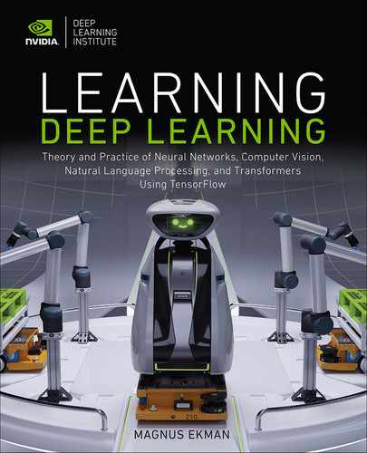
After these two changes, we have arrived at a model in which the first layer converts the inputs to word embeddings (i.e., it is an embedding layer) simply followed by a softmax (in reality, a hierarchical softmax) layer as the output layer. The only nonlinearity in the model is the softmax layer itself. These two modifications should address most of the computational complexity in the language model and thereby enable a larger training dataset. The model is illustrated in Figure 13-1.
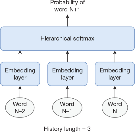
Figure 13-1 Simple model to create word embeddings. This model does not accurately represent the model from word2vec.
However, this is still not representative of what is used in the word2vec algorithm. The outlined model still has the limitation that it considers only historical words, so let us now move on to techniques that consider both historical and future words when training the embeddings.
Continuous Bag-of-Words Model
Extending our model to take future words into account is trivial. Instead of creating a training set from K consecutive words followed by the next word as the word to predict, we can select a word to predict and use a concatenation of the K preceding words and the K subsequent words as the input to the network. The most straightforward way to create our network would be to simply concatenate the embeddings corresponding to all the words. The input to the softmax layer would be 2×K×M, where 2×K is the number of words that we use as input and M is the embedding size for a single word. However, the way it is done in word2vec is to average the embeddings for the 2×K words and thereby produce a single embedding vector of size M. This architecture is shown in Figure 13-2, where K = 2.
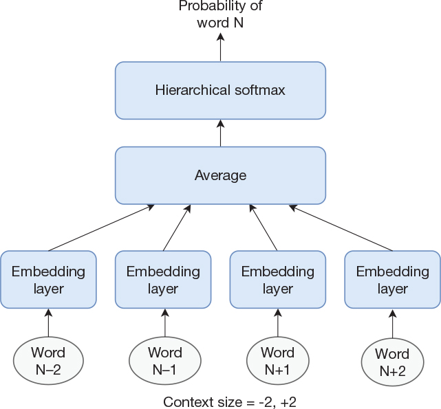
Figure 13-2 Architecture of the continuous bag-of-words model
Averaging the vectors has the effect that the order in which they are presented to the network does not matter, just as the order does not matter for a bag-of-words model. With that background, Mikolov, Chen, and colleagues (2013) named the model a continuous bag-of-words model, where the word continuous indicates that it is based on real-valued (i.e., continuous) word vectors. However, it is worth noting that the CBOW is not based on the entire document but on only the 2×K surrounding words.
The CBOW model was shown to outperform the embeddings created from an RNN-based language model in terms of how well it captures semantic structures in the dataset in addition to speeding up the training time significantly. However, the authors also discovered that a variation of the CBOW technique performed even better with respect to capturing semantics of the words. They named this variation the continuous skip-gram model, which is the model they later continued to optimize in favor of the CBOW model. The continuous skip-gram model is described next.
Continuous Skip-Gram Model
We have now described two major ways of creating embeddings. One is based on a model that uses historical words to predict a single word, and the other is based on a model that uses historical and future words to predict a single word. The continuous skip-gram model flips this around somewhat. Instead of predicting a single word based on its surrounding words (also known as the context), it tries to predict the surrounding words based on a single word. This might sound odd at first, but it results in the model becoming simpler. It takes a single word as its input and creates an embedding. This embedding is then fed to a fully connected softmax layer, which produces probabilities for each word in the vocabulary, but we now train it to output nonzero probabilities for multiple words (the words surrounding the input word) instead of just outputting a nonzero probability for a single word in the vocabulary. Figure 13-3 shows such a model.

Figure 13-3 Continuous skip-gram model
When discussing word2vec, context refers to the words surrounding the word in question. Note that when we discuss sequence-to-sequence networks in the next couple of chapters, the word context will have a different meaning.
Like CBOW, the model gets its name from a traditional model (skip-gram) but with the addition of continuous to again indicate that it deals with real-valued word vectors. A valid question is why this would work well, but we can use a similar line of reasoning as we did for why the language model would produce good embeddings. We have noted that words that have properties in common (e.g., they are synonyms or similar in some other way) often surround themselves with a similar set of words, as in our sentences “that is exactly what I mean” and “that is precisely what I mean.” If we train on both of these sentences, then our continuous skip-gram model is tasked with outputting a nonzero probability for the words that, is, what, I, and mean both when presented with exactly and when presented with precisely on its input. A simple way of achieving that is to produce embeddings in which those two words are close to each other in vector space. This explanation involves a fair amount of hand-waving, but remember that the model evolved on the basis of empirical studies. When you consider the history of how the models evolved, it is not hard to envision (although it was clearly still clever) how Mikolov, Chen, and colleagues (2013) experimented with different approaches and decided to try the continuous skip-gram once they had shown that the CBOW model worked well. Given that the continuous skip-gram model outperformed CBOW, they then continued to optimize the former, which is described next.
Although we say that “it is not hard to envision” that they came up with the continuous skip-gram model, it would not surprise us if they first tried a large number of other alternatives. After all, research is 10% inspiration and 90% perspiration, but that is often not clear when reading the published paper.
Optimized Continuous Skip-Gram Model to Further Reduce Computational Complexity
The original continuous skip-gram model used hierarchical softmax on its output, but in a subsequent paper, the algorithm was modified to make it even faster and simpler (Mikolov, Sutskever, et al., 2013). The overall observation was that both softmax and hierarchical softmax aim at computing correct probabilities for all words in the vocabulary, which is important for a language model, but as previously mentioned, the objective of word2vec is to create good word embeddings as opposed to a good language model. With that background, the algorithm was modified by replacing the softmax layer with a new mechanism named negative sampling. The observation was that instead of computing a true probability distribution across all the words in the vocabulary, it should be possible to produce good embeddings if we teach the network to just correctly identify the surrounding words, which are on the order of tens of words instead of tens of thousands of words. In addition, it is necessary to make sure that the network does not incorrectly produce high probabilities for words that are not part of the set of surrounding words.
We can achieve this in the following way. For each word K in the vocabulary, we maintain a single corresponding output neuron NK with a sigmoid activation function. For each training example X, we now serially train each of the neurons NX–2, NX–1, NX+1, NX+2 corresponding to the surrounding words (this example assumes that we considered four surrounding words). That is, we have converted the softmax problem into a series of classification problems. This is not sufficient, though. A naïve solution to this classification problem is for all output neurons to always output 1 because they are only sampled (trained) for the cases where their corresponding words are surrounding the input word. To get around this problem, we need to introduce some negative samples as well:
Given an input word, do the following:
1. Identify the output neurons corresponding to each surrounding word.
2. Train these neurons to output 1 when the network is presented with the input word.
3. Identify the output neurons corresponding to a number of random words that are not surrounding the input word.
4. Train these neurons to output 0 when the network is presented with the input word.
Table 13-1 illustrates this technique for the word sequence “that is exactly what I” with a context of four words (two before and two after) and using three negative samples per context word. Each training example (combination of input and output word) will train a separate output neuron.
Table 13-1 Training Examples for the Word Sequence “that is exactly what i” with Three Negative Samples per Context Word
INPUT WORD |
CONTEXT WORD |
OUTPUT WORD |
OUTPUT VALUE |
|---|---|---|---|
exactly |
N–2 |
that (actual context word) |
1.0 |
ball (random word) |
0.0 |
||
boat (random word) |
0.0 |
||
walk (random word) |
0.0 |
||
N–1 |
is (actual context word) |
1.0 |
|
blue (random word) |
0.0 |
||
bottle (random word) |
0.0 |
||
not (random word) |
0.0 |
||
N+1 |
what (actual context word) |
1.0 |
|
house (random word) |
0.0 |
||
deep (random word) |
0.0 |
||
computer (random word) |
0.0 |
||
N+2 |
i (actual context word) |
1.0 |
|
stupid (random word) |
0.0 |
||
airplane (random word) |
0.0 |
||
mitigate (random word) |
0.0 |
All in all, negative sampling further simplifies word2vec into an efficient algorithm, which has also been shown to produce good word embeddings.
Additional Thoughts on word2vec
Additional tweaks can be made to the algorithm as well, but we think that the preceding description captures the key points required to understand the big picture. Before moving on to the next topic, we provide some additional insights into the word2vec algorithm. We begin with a more detailed illustration of the network structure for readers who prefer visual descriptions and then move on to a matrix implementation for readers who prefer mathematical descriptions.
Figure 13-4 shows a network for training a word2vec model with a vocabulary of five words and an embedding size of three dimensions. The figure assumes that we are currently training based on a context word that is number four in the vocabulary (the other output neurons are ghosted).

Figure 13-4 The word2vec continuous skip-gram model
We present the input word to the network, which implies that one of the five inputs is of value 1 and all others are set to 0. Let us assume that the input word is number 0 in the vocabulary, so the input word 0 (Wd0) is set to 1 and all other inputs are set to 0. The embedding layer “computes” an embedding by multiplying all weights from node Wd0 by 1 and multiplying all other input weights by 0 (in reality, this is performed by indexing into a lookup table). We then compute the output of neuron y4 and ignore all others without any computation. After this forward pass, we do a backward pass and adjust the weights. Figure 13-4 highlights a noteworthy property. As previously described, the embedding layer contains K weights (denoted IWExy, where IWE refers to input word embedding) associated with each input word, where K is the size of the word vector. However, the figure shows that the output layer also contains K weights (denoted OWExy, where OWE refers to output word embedding) associated with each output word. By definition, the number of output nodes is the same as the number of input words. That is, the algorithm produces two embeddings for each word: one input embedding and one output embedding. In the original paper, the input embeddings were used, and the output embeddings were discarded, but Press and Wolf (2017) have shown that it can be beneficial to tie the input and output embeddings together using weight sharing.
In a model where the input and output weights are tied together, it is also possible to reason about how the embeddings for words in the same context relate to each other. Consider the mathematical operation used to compute the weighted sum for a single output neuron. It is the dot product of the word embedding for the input word and the word embedding for the output word, and we train the network to make this dot product get close to 1.0. The same holds true for all the output words in that same context. Now consider the condition needed for a dot product to result in a positive value. The dot product is computed by elementwise multiplication between the two vectors and then adding the results together. This sum tends to be positive if corresponding elements in both the vectors are nonzero and have the same sign (i.e., the vectors are similar). A straightforward way to achieve the training objective is to ensure that the word vectors for all words in the same context are similar to each other. Obviously, this does not guarantee that the produced word vectors express the desired properties, but it provides some further insight into why it is not entirely unexpected that the algorithm produces good word embeddings.
word2vec in Matrix Form
Another way of describing the mechanics of word2vec is to simply look at the mathematics that is performed. This description is influenced by one of the sections of the popular blog post “The Illustrated Word2vec” (Alammar, 2019). We start by creating two matrices, as shown in Figure 13-5. Both are of the same dimensions with N rows and M columns, where N is the number of words in the vocabulary and M is the desired embedding width. One matrix will be used for the central word (the input word), and the other matrix will be used for the surrounding words (the context).
Figure 13-5 Matrices with input and output embeddings
We now select a word (the central word) from our text as well as a number of words surrounding it. We look up the embedding for the central word from the input embeddings matrix (select a single row) and we look up the embeddings for the surrounding words from the output embeddings matrix. These are our positive samples (i.e., where the output value is 1 in the previously shown Table 13-1). We further randomly sample a number of additional embeddings from the output-embedding matrix. These are our negative samples (i.e., where the output value should be 0).
Now we simply compute the dot products between the selected input embedding and each of the selected output embeddings, apply the logistic sigmoid function to each of these dot products, and compare to the desired output value. We then adjust each of the selected embeddings using gradient descent, and then repeat this process for a different central word. In the end, the leftmost matrix in Figure 13-5 will contain our embeddings.
Wrapping Up word2vec
To wrap up the discussion about word2vec, according to our understanding, several people struggle with the mechanics of the algorithm and how it relates to bag-of-words and traditional skip-gram, as well as with why the algorithm produces good word embeddings. We hope that we have brought clarity to the mechanics of the algorithms. The relationship to bag-of-words and skip-grams is just that there are some aspects of some steps of the word2vec algorithms that are related to these traditional algorithms, and consequently, Mikolov, Chen, and colleagues (2013) decided to name them after these techniques, but we would like to emphasize that they are completely different beasts. The traditional skip-gram is a language model, and the bag-of-words is a way of summarizing a document, whereas the continuous bag-of-words and continuous skip-gram models in word2vec are algorithms that produce word embeddings. Finally, as to the question of why word2vec produces good word embeddings, we hope that we have provided some insight into why it makes sense, but as far as we understand it, it is more of a result of discoveries, trial-and-error, observations, and refinements than a top-down engineering effort.
We summarize our understanding of the evolution leading up to the word2vec algorithm in Figure 13-6. The first few steps are more about neural language models than word embeddings, but as described, language models played a critical part in the process of developing word embeddings. The figure also illustrates how word2vec was not a single step but a process of gradual refinements.
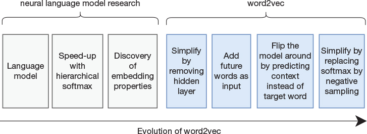
Figure 13-6 Evolution of neural language models into word2vec
The release of the word2vec implementation spawned considerable interest in word embedding research that has resulted in multiple alternative embedding schemes. One such scheme is the GloVe embeddings, which we now explore with a programming example.
Programming Example: Exploring Properties of GloVe Embeddings
About a year after word2vec was published, Pennington, Socher, and Manning (2014) published “GloVe: Global Vectors for Word Representation.” GloVe is an algorithm mathematically engineered to create well-behaved word embeddings. In particular, the goal is that the embeddings capture syntactic and semantic relationships between words. We do not describe the details of how GloVe works, as the mathematics/statistics needed to understand it is more than we want to require from readers of this book. However, we strongly recommend that anyone who wants to get serious about word embedding research (as opposed to just using word embeddings) acquire the necessary skills to understand the GloVe paper. The paper also provides additional information about why word2vec produces sane embeddings. The embeddings are available for download and are contained in a text file in which each line represents a word embedding. The first element is the word itself followed by the vector elements separated by blank spaces.
Code Snippet 13-1 contains two import statements and a function to read the embeddings. The function simply opens the file and reads it line by line. It splits each line into its elements. It extracts the first element, which represents the word itself, and then creates a vector from the remaining elements and inserts the word and the corresponding vector into a dictionary, which serves as the return value of the function.
Code Snippet 13-1 Loading GloVe Embeddings from File
import numpy as np
import scipy.spatial

# Read embeddings from file.
def read_embeddings():
    FILE_NAME = '../data/glove.6B.100d.txt'
    embeddings = {}
    file = open(FILE_NAME, 'r', encoding='utf-8')
    for line in file:
        values = line.split()
        word = values[0]
        vector = np.asarray(values[1:],
                            dtype='float32')
        embeddings[word] = vector
    file.close()
    print('Read %s embeddings.' % len(embeddings))
    return embeddings
Code Snippet 13-2 implements a function that computes the cosine distance between a specific embedding and all other embeddings. It then prints the n closest ones. This is similar to what was done in Chapter 12, but we are using cosine distance instead of Euclidean distance to demonstrate how to do that. Euclidean distance would also have worked fine, but the results would sometimes be different because the GloVe vectors are not normalized.
Code Snippet 13-2 Function to Identify and Print the Three Words That Are Closest in Vector Space, Using Cosine Distance
def print_n_closest(embeddings, vec0, n):
    word_distances = {}
    for (word, vec1) in embeddings.items():
        distance = scipy.spatial.distance.cosine(
            vec1, vec0)
        word_distances[distance] = word
    # Print words sorted by distance.
    for distance in sorted(word_distances.keys())[:n]:
        word = word_distances[distance]
        print(word + ': %6.3f' % distance)
Using these two functions, we can now retrieve word embeddings for arbitrary words and print out words that have similar embeddings. This is shown in Code Snippet 13-3, where we first read call read_embeddings() and then retrieve the embeddings for hello, precisely, and dog and call print_n_closest() on each of them.
Code Snippet 13-3 Printing the Three Closest Words to hello, precisely, and dog
embeddings = read_embeddings()

lookup_word = 'hello'
print('
Words closest to ' + lookup_word)
print_n_closest(embeddings,
                embeddings[lookup_word], 3)

lookup_word = 'precisely'
print('
Words closest to ' + lookup_word)
print_n_closest(embeddings,
                embeddings[lookup_word], 3)

lookup_word = 'dog'
print('
Words closest to ' + lookup_word)
print_n_closest(embeddings,
                embeddings[lookup_word], 3)
The resulting printouts follow. We see that the vocabulary consists of 400,000 words, and as expected, the closest word to each lookup word is the lookup word itself (there is zero distance between hello and hello). The other two words close to hello are goodbye and hey. The two words close to precisely are exactly and accurately, and the two words close to dog are cat and dogs. Overall, this demonstrates that the GloVe embeddings do capture semantics of the words.
Read 400000 embeddings.

Words closest to hello
hello:  0.000
goodbye:  0.209
hey:  0.283

Words closest to precisely
precisely:  0.000
exactly:  0.147
accurately:  0.293
Words closest to dog
dog:  0.000
cat:  0.120
dogs:  0.166
Using NumPy, it is also trivial to combine multiple vectors using vector arithmetic and then print out words that are similar to the resulting vector. This is demonstrated in Code Snippet 13-4, which first prints the words closest to the word vector for king and then prints the words closest to the vector resulting from computing (king – man + woman).
Code Snippet 13-4 Example of Word Vector Arithmetic
lookup_word = 'king'
print('
Words closest to ' + lookup_word)
print_n_closest(embeddings,
                embeddings[lookup_word], 3)

lookup_word = '(king - man + woman)'
print('
Words closest to ' + lookup_word)
vec = embeddings['king'] - embeddings[
    'man'] + embeddings['woman']
print_n_closest(embeddings, vec, 3)
It yields the following output:
Words closest to king
king:  0.000
prince:  0.232
queen:  0.249

Words closest to (king - man + woman)
king:  0.145
queen:  0.217
monarch:  0.307
We can see that the closest word to king (ignoring king itself) is prince, followed by queen. We also see that the closest word to (king – man + woman) is still king, but the second closest is queen; that is, the calculations resulted in a vector that is more on the female side, since queen is now closer than prince. Without diminishing the impact of the king/queen discovery, we recognize that the example provides some insight into how the (king – man + woman) property could be observed in embeddings resulting from a relatively simple model. Given that king and queen are closely related, they were likely close to each other from the beginning, and not much tweaking was needed to go from king to queen. For example, from the printouts, we can see that the distance to queen only changed from 0.249 (distance between queen and king) to 0.217 (distance between queen and the vector after arithmetic).
A possibly more impressive example is shown in Code Snippet 13-5, where we first print the words closest to sweden and madrid and then print the words closest to the result from the computation (madrid – spain + sweden).
Code Snippet 13-5 Vector Arithmetic on Countries and Capital Cities
lookup_word = 'sweden'
print('
Words closest to ' + lookup_word)
print_n_closest(embeddings,
                embeddings[lookup_word], 3)

lookup_word = 'madrid'
print('
Words closest to ' + lookup_word)
print_n_closest(embeddings,
                embeddings[lookup_word], 3)

lookup_word = '(madrid - spain + sweden)'
print('
Words closest to ' + lookup_word)
vec = embeddings['madrid'] - embeddings[
    'spain'] + embeddings['sweden']
print_n_closest(embeddings, vec, 3)
As you can see in the following output, the words closest to Sweden are the neighboring countries Denmark and Norway. Similarly, the words closest to Madrid are Barcelona and Valencia, two other significant Spanish cities. Now, removing Spain from Madrid (its capital) and instead adding Sweden results in the Swedish capital city of Stockholm, which seemingly came out of nowhere as opposed to the king/queen example where queen was already closely related to king.
Words closest to sweden
sweden:  0.000
denmark:  0.138
norway:  0.193

Words closest to madrid
madrid:  0.000
barcelona:  0.157
valencia:  0.197

Words closest to (madrid - spain + sweden)
stockholm:  0.271
sweden:  0.300
copenhagen:  0.305
In reality, it turns out that if we expand the list of words close to madrid and sweden, then stockholm does show up as number 18 on the sweden list (and 377 on the madrid list), but we still find it impressive how the equation correctly identifies it as the top 1.
Concluding Remarks on word2vec and GloVe
In these past two chapters, we have seen that it is possible to learn word embeddings jointly with a DL model or learn the word embeddings in isolation. Algorithms such as word2vec and GloVe are not DL algorithms, although word2vec is inspired by, and to some extent evolved from, a neural language model. Still, the embeddings produced from these algorithms are useful when applying DL models to natural language.
A valid question is whether it is best to use prelearned embeddings in a transfer learning setting or to learn the embeddings jointly with the DL model, and the answer is that it is application dependent. There are cases in which it is useful to use pretrained embeddings that are derived from a large dataset, especially if your dataset on the end task is not that big. In other cases, it is better to learn the embeddings jointly with the model. One example would be a use case where the pretrained embeddings do not capture use case–specific relationships. Another one is if you are working with natural language translation to a rare language and you simply do not have access to pretrained embeddings.
Since GloVe was published, there have been additional improvements in the space of word embeddings. They have been extended with capabilities to handle words that were not present in the training vocabulary. They have also been extended to handle cases where a single word can have two different meanings depending on the context in which it is used. We describe more details about these types of embeddings in Appendix C. If you are very interested in word embeddings, consider reading it now. We recommend that most readers just continue reading the book in order. Chapter 14, “Sequence-to-Sequence Networks and Natural Language Translation,” uses word embeddings and other concepts we have discussed to build a network for natural language translation.
We have not brought up the topic of science fiction movies for a few chapters, so we feel that it is time to do another farfetched analogy. When watching the 2016 movie Arrival, where Amy Adams plays a linguist who is asked to try to learn an alien language, we think that it would have been very cool if they had slipped in a reference to word2vec. For example, when trying to persuade Adams’s character to take on the case, they could have said, “We have already run word2vec on the aliens’ Wikipedia database, and it didn’t uncover any compositional relationships but just some weird temporal relationships both forward and backward.”
Perhaps the reason this was not done is that it is one of the cases where science was ahead of fiction?!