
The ROS image pipeline is run with the image_proc package. It provides all the conversion utilities to obtain monochrome and color images from the RAW images acquired from the camera. In the case of FireWire cameras, which may use a Bayer pattern to code the images (actually in the sensor itself), it debayers them to obtain the color images. Once you have calibrated the camera, the image pipeline takes the CameraInfo messages, which contain that information, and rectifies the images. Here, rectification means to un-distort the images, so it takes the coefficients of the distortion model to correct the radial and tangential distortion.
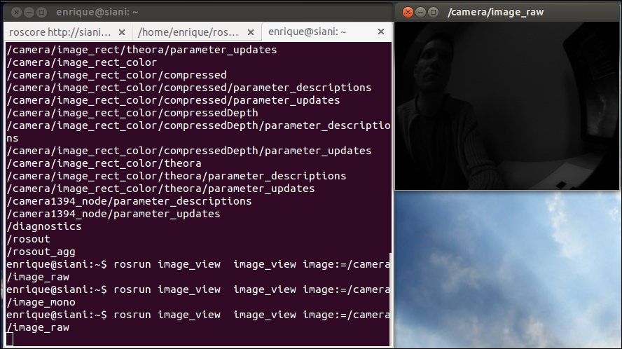
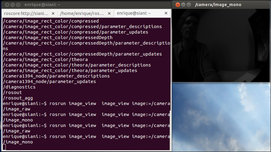
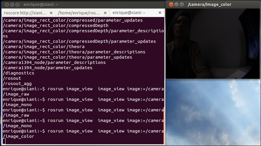
As a result, you will see more topics for your camera in its namespace. In the following screenshots, you can see the image_raw, image_mono, and image_color topics, which display the RAW, monochrome, and color images, respectively:
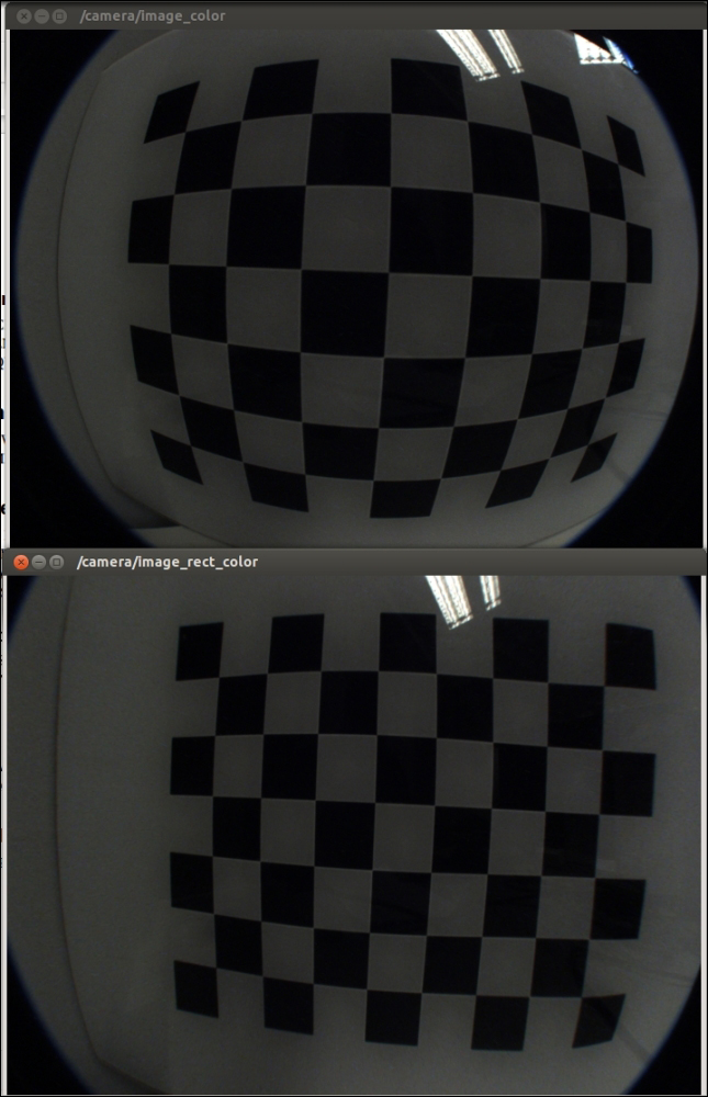
The rectified images are provided in monochrome and color in the image_rect and image_rect_color topics. In the following image, we compare the uncalibrated, distorted RAW images with the rectified ones. You can see the correction because the pattern shown in the screenshots has straight lines only in the rectified images, particularly in areas far from the center (principle point) of the image (sensor):
You can see all the topics available with rostopic list or rqt_graph, which include the image_transport topics as well.
You can view the image_raw topic of a monocular camera directly with the following command:
$ roslaunch chapter5_tutorials camera.launch view:=true
It can be changed to see other topics, but for these cameras, the RAW images are already in color. However, in order to see the rectified ones, use image_rect_color with image_view or rqt_image_view, or change the launch file. The image_proc node is used to make all these topics available. The following code shows this:
<node ns="$(arg camera)" pkg="image_proc" type="image_proc" name="image_proc"/>
In the case of stereo cameras, we have the same for the left-hand side and right-hand side cameras. However, there are specific visualization tools for them because we can use the left-hand side and right-hand side images to compute and see the disparity image. An algorithm uses stereo calibration and the texture of both images to estimate the depth of each pixel, which is the disparity image. To obtain good results, we must tune the algorithm that computes such an image. In the next screenshot, we see the left-hand side, right-hand side, and disparity images as well as rqt_reconfiguire for stereo_image_proc, which is the node that builds the image pipeline for stereo images; in the launch file, we only need the following lines:
<node ns="$(arg camera)" pkg="stereo_image_proc" type="stereo_image_proc"
    name="stereo_image_proc" output="screen">
  <rosparam file="$(arg params_disparity)"/>
</node>
It requires the disparity parameters, which can be set with rqt_reconfigure as shown in the following screenshot and saved with rosparam dump /stereo/stereo_image_proc:
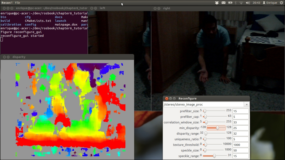
We have good values for the environment used in this book's demonstration in the config/camera_stereo/disparity.yaml parameters file. This is shown in the following code:
{correlation_window_size: 33, disparity_range: 32, min_disparity: 25, prefilter_cap: 5,
  prefilter_size: 15, speckle_range: 15, speckle_size: 50, texture_threshold: 1000,
  uniqueness_ratio: 5.0}
However, these parameters depend a lot on the calibration quality and the environment. You should adjust it to your experiments. It takes time and it is quite tricky, but you can follow the next guidelines. Basically, you start by setting a disparity_range value that makes enough blobs appear. You also have to set min_disparity, so you see areas covering the whole range of depths (from red to blue/purple). Then, you can fine-tune the result, setting speckle_size, to remove small, noisy blobs. Also, modify uniqueness_ratio and texture_threshold to have larger blobs. The correlation_window_size is also important since it affects the detection of initial blobs.
If it becomes very difficult to obtain good results, you might have to recalibrate or use better cameras for your environment and lighting conditions. You can also try it in another environment or with more light. It is important that you have texture in the environment; for example, from a flat, white wall, you cannot find any disparity. Also, depending on the baseline, you cannot retrieve depth information very close to the camera. For stereo navigation, it is better to have a large baseline, say 12 cm or more. We use it here because, later, we will try visual odometry. However, with this setup, we only have depth information one meter apart from the cameras. With a smaller baseline, on the contrary, we can obtain depth information from closer objects. This is bad for navigation because we lose resolution far away, but it is good for perception and grasping.
As far as calibration problems go, you can check your calibration results with the cameracheck.py node, which is integrated in both the monocular and stereo camera launch files:
$ roslaunch chapter5_tutorials camera.launch view:=true check:=true
$ roslaunch chapter5_tutorials camera_stereo.launch view:=true check:=true
For the monocular camera, our calibration yields this RMS error (see more in calibration/camera/cameracheck-stdout.log):
Linearity RMS Error: 1.319 Pixels      Reprojection RMS Error: 1.278 Pixels
Linearity RMS Error: 1.542 Pixels      Reprojection RMS Error: 1.368 Pixels
Linearity RMS Error: 1.437 Pixels      Reprojection RMS Error: 1.112 Pixels
Linearity RMS Error: 1.455 Pixels      Reprojection RMS Error: 1.035 Pixels
Linearity RMS Error: 2.210 Pixels      Reprojection RMS Error: 1.584 Pixels
Linearity RMS Error: 2.604 Pixels      Reprojection RMS Error: 2.286 Pixels
Linearity RMS Error: 0.611 Pixels      Reprojection RMS Error: 0.349 Pixels
For the stereo camera, we have epipolar error and the estimation of the cell size of the calibration pattern (see more in calibration/camera_stereo/cameracheck-stdout.log):
epipolar error: 0.738753 pixels   dimension: 0.033301 m
epipolar error: 1.145886 pixels   dimension: 0.033356 m
epipolar error: 1.810118 pixels   dimension: 0.033636 m
epipolar error: 2.071419 pixels   dimension: 0.033772 m
epipolar error: 2.193602 pixels   dimension: 0.033635 m
epipolar error: 2.822543 pixels   dimension: 0.033535 m
To obtain these results, you only have to show the calibration pattern to the camera/s; that is the reason why we also pass view:=true to the launch files. An RMS error greater than 2 pixels is quite large; we have something around it, but remember that these are very low-cost cameras. Something below a 1 pixel error is desirable. For the stereo pair, the epipolar error should also be lower than 1 pixel; in our case, it is still quite large (usually greater than 3 pixels), but we still can do many things. Indeed, the disparity image is just a representation of the depth of each pixel shown with the stereo_view node. We also have a 3D point cloud that can be visualized texturized with rviz. We will see this in the following demonstrations, doing visual odometry.