6

Diving Deep with Table Calculations

Table calculations are one of the most powerful features in Tableau. They enable solutions that really couldn’t be achieved any other way (short of writing a custom application or complex custom SQL scripts!). The features include the following:

• They make it possible to use data that isn’t structured well and still get quick results without waiting for someone to fix the data at the source.
• They make it possible to compare and perform secondary aggregations and work across values within a visualization.
• They open incredible possibilities for analysis and creative approaches to solving problems, highlighting insights, or improving the user experience.

Table calculations range in complexity, from incredibly easy to create (a couple of clicks) to extremely complex (requiring an understanding of addressing, partitioning, and data densification, for example). We’ll start off simple and move toward complexity in this chapter. The goal is to gain a solid foundation in creating and using table calculations, understanding how they work, and looking at some examples of how they can be used. We’ll consider these topics:

• An overview of table calculations
• Quick table calculations
• Relative versus fixed
• Scope and direction
• Addressing and partitioning
• Custom table calculations
• Practical examples

The examples in this chapter will return to the sample Superstore data that we used in the first chapter. To follow along with the examples, use the Chapter 06 Starter.twbx workbook.

An overview of table calculations

Table calculations are different from all other calculations in Tableau. Row-level, aggregate calculations, and level of detail (LOD) expressions, which we explored in the previous chapters, are performed as part of the query to the data source. If you were to examine the queries sent to the data source by Tableau, you’d find the code for your calculations translated into whatever implementation of SQL the data source used.

Table calculations, on the other hand, are performed after the initial query. Here’s a diagram that demonstrates how aggregated results are stored in Tableau’s cache:

Figure 6.1: Table calculations are computed in Tableau’s cache of aggregated data

Table calculations are performed on the aggregate table of data in Tableau’s cache right before the data visualization is rendered. As we’ll see, this is important to understand for multiple reasons, including the following:

• Aggregation: Table calculations operate on aggregate data. You cannot reference a field in a table calculation without referencing the field as an aggregate.
• Filtering: Regular filters will be applied before table calculations. This means that table calculations will only be applied to data returned from the source to the cache. You’ll need to avoid filtering any data necessary for the table calculation.
• Table calculation filtering (sometimes called late filtering): Table calculations used as filters will be applied after the aggregate results are returned from the data source. The order is important: row-level and aggregate filters are applied first, the aggregate data is returned to the cache, and then the table calculation is applied as a filter that effectively hides data from the view. This allows some creative approaches to solving certain kinds of problems that we’ll consider in some of the examples later in the chapter.
• Performance: If you are using a live connection to an enterprise database server, then row-level and aggregate-level calculations will be taking advantage of enterprise-level hardware. Table calculations are performed in the cache, which means they will be performed on whatever machine is running Tableau.

You will not likely need to be concerned if your table calculations are operating on a dozen or even hundreds of rows of aggregate data, or if you anticipate publishing to a powerful Tableau server. However, if you are getting back hundreds of thousands of rows of aggregate data on your local machine, then you’ll need to consider the performance of your table calculations. At the same time, there are cases where table calculations might be used to avoid an expensive filter or calculation at the source.

With this overview of table calculations in mind, let’s jump into understanding some options for creating table calculations.

Creating and editing table calculations

There are several ways to create table calculations in Tableau, including:

• Using the drop-down menu for any active field used as a numeric aggregate in the view, selecting Quick Table Calculation and then the desired calculation type
• Using the drop-down menu for any active field that is used as a numeric aggregate in the view, selecting Add Table Calculation, then selecting the calculation type and adjusting any desired settings
• Creating a calculated field and using one or more table calculation functions to write your own custom table calculations

The first two options create a quick table calculation, which can be edited or removed using the drop-down menu on the field and by selecting Edit Table Calculation... or Clear Table Calculation. The third option creates a calculated field, which can be edited or deleted like any other calculated field.

A field on a shelf in the view that is using a table calculation, or which is a calculated field using table calculation functions, will have a delta symbol icon () visible, as follows.

Following is a snippet of an active field without a table calculation:

Figure 6.2: An active field without a table calculation applied

Following is the active field with a table calculation:

Figure 6.3: An active field with a table calculation applied includes the delta symbol

Most of the examples in this chapter will utilize text tables/cross-tab reports as these most closely match the actual aggregate table in the cache. This makes it easier to see how the table calculations are working.

Table calculations can be used in any type of visualization. However, when building a view that uses table calculations, especially more complex ones, try using a table with all dimensions on the Rows shelf and then adding table calculations as discrete values on Rows to the right of the dimensions. Once you have all the table calculations working as desired, you can rearrange the fields in the view to give you the appropriate visualization. This approach approximates the way table calculations are computed in the aggregate table in Tableau’s cache and allows you to think through how the various dimensions and aggregations work together and impact your calculations.

We’ll now move from the concept of creating table calculations to some examples.

Quick table calculations

Quick table calculations are predefined table calculations that can be applied to fields used as measures in the view. These calculations include common and useful calculations such as Running Total, Difference, Percent Difference, Percent of Total, Rank, Percentile, Moving Average, YTD Total (year-to-date total), Compound Growth Rate, Year over Year Growth, and YTD Growth. You’ll find applicable options on the drop-down list on a field used as a measure in the view, as shown in the following screenshot:

Figure 6.4: Using the dropdown, you can create a quick table calculation from an aggregate field in the view

Consider the following example using the sample Superstore Sales data:

Figure 6.5: The first SUM(Sales) field is a normal aggregate. The second has a quick table calculation of Running Total applied

Here, Sales over time is shown. Sales has been placed on the Rows shelf twice and the second SUM(Sales) field has had the running total quick table calculation applied. Using the quick table calculation meant it was unnecessary to write any code.

You can actually see the code that the quick table calculation uses by double-clicking the table calculation field in the view. This turns it into an ad hoc calculation. You can also drag an active field with a quick table calculation applied to the data pane, which will turn it into a calculated field that can be reused in other views.

The following table demonstrates some of the quick table calculations:

Figure 6.6: Sales in the first column is simply the SUM(Sales). The three additional columns show various table calculations applied (Running Sum, Difference, Rank)

Fundamental table calculation concepts

Although it is quite easy to create quick table calculations, it is essential to understand some fundamental concepts. We’ll take a look at these next, starting with the difference between relative and fixed table calculations.

Relative versus fixed

We’ll look at the details shortly, but first, it is important to understand that table calculations may be computed in one of the following two ways:

• Relative: The table calculation will be computed relative to the layout of the table. They might move across or down the table. Rearranging dimensions in a way that changes the table will change the table calculation results. As we’ll see, the key for relative table calculations is scope and direction. When you set a table calculation to use a relative computation, it will continue to use the same relative scope and direction, even if you rearrange the view.

  The term relative here is different from Relative To that appears in the UI for some quick table calculations.

• Fixed: The table calculation will be computed using one or more dimensions. Rearranging those dimensions in the view will not change the computation of the table calculation. Here, the scope and direction remain fixed to one or more dimensions, no matter where they are moved within the view. When we talk about fixed table calculations, we’ll focus on the concepts of partitioning and addressing.

You can see these concepts in the user interface. The following is the Table Calculation editor that appears when you select Edit Table Calculation from the menu of a table calculation field:

Figure 6.7: The Edit Table Calculation UI demonstrates the difference between Relative and Fixed table calculations

We’ll explore the options and terms in more detail, but for now, notice the options that relate to specifying a table calculation that is computed relative to rows and columns, and options that specify a table calculation that is computed fixed to certain dimensions in the view.

Next, we’ll look at scope and direction, which describe how relative table calculations operate.

Scope and direction

Scope and direction are terms that describe how a table calculation is computed relative to the table. Specifically, scope and direction refer to the following:

• Scope: The scope defines the boundaries within which a given table calculation can reference other values.
• Direction: The direction defines how the table calculation moves within the scope.

You’ve already seen table calculations being calculated in Table (across) (the running sum of sales over time in Figure 6.5) and Table (down) (in Figure 6.6). In these cases, the scope was the entire table and the direction was either across or down. For example, the running total calculation ran across the entire table, adding subsequent values as it moved from left to right.

To define the scope and direction for a table calculation, use the drop-down menu for the field in the view and select Compute Using. You will get a list of options that vary slightly depending on the location of dimensions in the view. The first of the options listed allows you to define the scope and direction relative to the table. After the option for Cell, you will see a list of dimensions present in the view. We’ll look at those in the next section.

The options for scope and direction relative to the table are as follows:

• Scope options: Table, pane, and cells
• Direction options: Down, across, down then across, across then down

In order to understand these options, consider the following example:

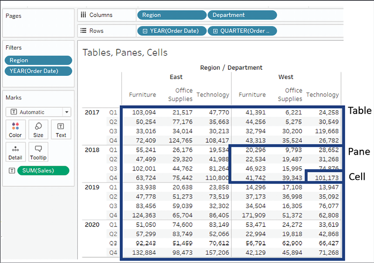
Figure 6.8: The difference between table, pane, and cell in the view

When it comes to the scope of table calculations, Tableau makes the following distinctions:

• The table is the entire set of aggregate data.
• The pane is a smaller section of the entire table. Technically, it is defined by the penultimate level of the table; that is, the next-to-last dimension on the Rows and/or Columns shelf defines the pane. In the preceding screenshot, you can see that the intersection of Year on rows and Region on columns defines the panes (one of eight is highlighted in the view).
• The cell is defined by the lowest level of the table. In this view, the intersection of one Department within a Region and one Quarter within a Year is a single cell (one of 96 is highlighted in the view).

The bounded areas in the preceding screenshot are defined by the scope. Scope (and, as we’ll see, also partition) defines windows within the data that contain various table calculations. Window functions, such as WINDOW_SUM() in particular, work within the scope of these windows.

In order to see how scope and direction work together, let’s work through a few examples. We’ll start by creating our own custom table calculations. Create a new calculated field named Index containing the code Index().

Index() is a table calculation function that has an initial value of 1 and increments by one as it moves in a given direction and within a given scope. There are many practical uses for Index(), but we’ll use it here because it is easy to see how it is moving for a given scope and direction.

Create the table as shown in Figure 6.8, with YEAR(Order Date) and QUARTER(Order Date) on Rows and Region and Department on Columns. Instead of placing Sales in the view, add the newly created Index field to the Text shelf. Then, experiment using the drop-down menu on the Index field and select Compute Using to cycle through various scope and direction combinations. In the following examples, we’ve only kept the East and West regions and two years, 2015 and 2016:

• Table (across): This is Tableau’s default when there are columns in the table. Notice in the following how Index increments across the entire table:

Figure 6.9: Table (across)

• Table (down): When using table (down), Index increments down the entire table:

Figure 6.10: Table (down)

• Table (across then down): This increments Index across the table, then steps down, continues to increment across, and repeats for the entire table:

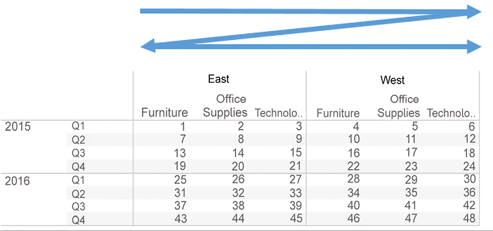
Figure 6.11: Table (across then down)

• Pane (across): This defines a boundary for Index and causes it to increment across until it reaches the pane boundary, at which point the indexing restarts:

Figure 6.12: Pane (across)

• Pane (down): This defines a boundary for Index and causes it to increment down until it reaches the pane boundary, at which point the indexing restarts:

Figure 6.13: Pane (down)

• Pane (across then down): This allows Index to increment across the pane and continue by stepping down. The pane defines the boundary here:

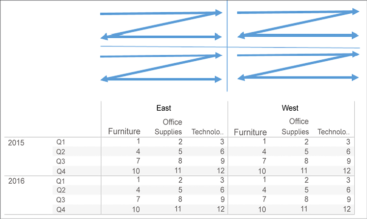
Figure 6.14: Pane (across then down)

You may use scope and direction with any table calculation. Consider how a running total or percentage difference would be calculated using the same movement and boundaries shown here. Keep experimenting with different options until you feel comfortable with how scope and direction work.

Scope and direction operate relative to the table, so you can rearrange fields, and the calculation will continue to work in the same scope and direction. For example, you could swap Year of Order Date with Department and still see Index calculated according to the scope and direction you defined.

Next, we’ll take a look at the corresponding concept for table calculations that are fixed to certain dimensions.

Addressing and partitioning

Addressing and partitioning are very similar to scope and direction but are most often used to describe how table calculations are computed with absolute reference to certain fields in the view. With addressing and partitioning, you define which dimensions in the view define the addressing (direction) and all others define the partitioning (scope).

Using addressing and partitioning gives you much finer control because your table calculations are no longer relative to the table layout, and you have many more options for fine-tuning the scope, direction, and order of the calculations.

To begin to understand how this works, let’s consider a simple example. Using the preceding view, select Edit table calculation from the drop-down menu of the Index field on Text. In the resulting dialog box, check Department under Specific Dimensions.

The result of selecting Department is as follows:

Figure 6.15: Setting the table calculation to Compute Using Specific Dimensions uses addressing and partitioning

You’ll notice that Tableau is computing Index along (in the direction of) the checked dimension, Department. In other words, you have used Department for addressing, so each new department increments the index. All other unchecked dimensions in the view are implicitly used for partitioning; that is, they define the scope or boundaries at which the index function must restart. As we saw with scope, these boundaries are sometimes referred to as a window.

The preceding view looks identical to what you would see if you set Index to compute using Pane (across). However, there is a major difference. When you use Pane (across), Index is always computed across the pane, even if you rearrange the dimensions in the view, remove some, or add others.

But when you compute using a dimension for addressing, the table calculation will always compute using that dimension. Removing that dimension will break the table calculation (the field will turn red with an exclamation mark) and you’ll need to edit the table calculation via the drop-down menu to adjust the settings. If you rearrange dimensions in the view, Index will continue to be computed along the Department dimension.

Here, for example, is the result of clicking the Swap Rows and Columns button in the toolbar:

Figure 6.16: Swapping Rows and Columns does not change how this table calculation was computed as it is fixed to the dimensions rather than the table layout

Notice that Index continues to be computed along Department even though the entire orientation of the table has changed. To complete the following examples, we’ll undo the swap of rows and columns to return our table to its original orientation.

Let’s consider a few other examples of what happens when you add additional dimensions. For example, if you check Quarter of Order Date, you’ll see Tableau highlight a partition defined by Region and Year of Order Date, with Index incrementing by the addressing fields of Quarter of Order Date and then Department:

Figure 6.17: Adding dimensions alters the table calculation’s behavior. One of the resulting partitions is highlighted

If you were to select Department and Year of Order Date as the addressing of Index, you’d see a single partition defined by Region and Quarter of Order Date, like this:

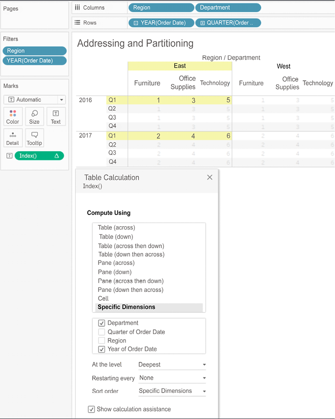
Figure 6.18: Changing the checked dimensions alters the table calculation’s behavior. One of the resulting partitions is highlighted

You’ll notice, in this view, that Index increments for every combination of Year of Order Date and Department within the partition of Quarter of Order Date and Region.

These are a few of the other things to consider when working with addressing and partitioning:

• You can specify the sort order. For example, if you wanted Index to increment according to the value of the sum of sales, you could use the drop-down list at the bottom of the table calculation editor to define a custom sort based on the sum of sales.
• The At the Level option in the edit table calculation dialog box allows you to specify a level at which the table calculations are performed. Most of the time, you’ll leave this set at Deepest (which is the same as setting it to the bottom-most dimension), but occasionally, you might want to set it at a different level if you need to keep certain dimensions from defining the partition but need the table calculation to be applied at a higher level. You can also reorder the dimensions by dragging and dropping within the checkbox list of Specific Dimensions.
• The Restarting Every option effectively makes the selected field, and all dimensions in the addressing above that selected field, part of the partition, but allows you to maintain the fine-tuning of the ordering.
• Dimensions are the only kinds of fields that can be used in addressing; however, a discrete (blue) measure can be used to partition table calculations. To enable this, use the drop-down menu on the field and uncheck Ignore in Table Calculations.

Take some time to experiment with various options and become comfortable with how addressing and partitioning work. Next, we’ll look at how to write our own custom table calculations.

Custom table calculations

Before we move on to some practical examples, let’s briefly discuss how to write your own table calculations, instead of using quick table calculations. You can see a list of available table calculation functions by creating a new calculation and selecting Table Calculation from the drop-down list under Functions.

For each of the examples, we’ll set Compute Using | Category. This means that Department will be the partition.

You can think of table calculations broken down into several categories. The following table calculations can be combined and even nested just like other functions.

Meta table functions

These are the functions that give you information about partitioning and addressing. These functions also include Index, First, Last, and Size:

• Index gives an increment as it moves along the addressing within the partition
• First gives the offset from the first row in the partition, so the first row in each partition is 0, the next row is -1, then -2, and so on
• Last gives the offset to the last row in the partition, so the last row in each partition is 0, the next-to-last row is 1, then 2, and so on
• Size gives the size of the partition

The following screenshot illustrates the various functions:

Figure 6.19: Meta table calculations

Index, First, and Last are all affected by scope/partition and direction/addressing, while Size will give the same result at each address of the partition, no matter what direction is specified.

Lookup and previous value

The first of these two functions gives you the ability to reference values in other rows, while the second gives you the ability to carry forward values.

Notice from the following screenshot that direction is very important for these two functions:

Figure 6.20: Lookup and Previous_Value functions (though Previous_Value includes some additional logic described below)

Both calculations are computed using the addressing of Category (so Department is the partition).

Here, we’ve used the code Lookup(ATTR([Category]), -1), which looks up the value of the category in the row offset by -1 from the current one. The first row in each partition gets a NULL result from the lookup (because there isn’t a row before it).

For Previous_Value, we used this code:

Previous_Value("") + "," + ATTR([Category]) 

Notice that in the first row of each partition, there is no previous value, so Previous_Value() simply returned what we specified as the default: an empty string. This was then concatenated together with a comma and the category in that row, giving us the value Bookcases.

IF LEN(Previous_Value("")) == 0 
THEN ATTR([Category])
ELSE Previous_Value("") + "," + ATTR([Category])
END

In the second row, Bookcases is the previous value, which gets concatenated with a comma and the category in that row, giving us the value Bookcases, Chairs & Chairmats, which becomes the previous value in the next row. The pattern continues throughout the partition and then restarts in the partition defined by the Office Supplies department.

Running functions

These functions run along direction/addressing and include Running_Avg(), Running_Count(), Running_Sum(), Running_Min(), and Running_Max(), as follows:

Figure 6.21: Running Functions

Notice that Running_Sum(SUM[Sales])) continues to add the sum of sales to a running total for every row in the partition. Running_Min(SUM[Sales])) keeps the value of the sum of sales if it is the smallest value it has encountered so far as it moves along the rows of the partition.

Window functions

These functions operate across all rows in the partition at once and essentially aggregate the aggregates. They include Window_Sum, Window_Avg, Window_Max, and Window_Min, among others, as shown in the following screenshot:

Figure 6.22: Examples of Window functions

Window_Sum(SUM([Sales]) adds up the sums of sales within the entire window (in this case, for all categories within the department). Window_Max(SUM([Sales]) returns the maximum sum of sales within the window.

You may pass optional parameters to window functions to further limit the scope of the window. The window will always be limited to, at most, the partition.

Rank functions

These functions provide various ways to rank based on aggregate values. There are multiple variations of rank, which allow you to decide how to deal with ties (equal values) and how dense the ranking should be, as shown in the following screenshot:

Figure 6.23: Examples of rank functions

The Rank(SUM([Sales]) calculation returns the rank of the sum of sales for categories within the department.

Script functions

These functions allow integration with the R analytics platform or Python, either of which can incorporate simple or complex scripts for everything from advanced statistics to predictive modeling. We’ll consider various examples of this functionality in Chapter 13, Integrating Advanced Features: Extensions, Scripts, and AI.

The Total function

The Total function deserves its own category because it functions a little differently from the others. Unlike the other functions, which work on the aggregate table in the cache, Total will re-query the underlying source for all the source data rows that make up a given partition. In most cases, this will yield the same result as a window function.

For example, Total(SUM([Sales])) gives the same result as Window_Sum(SUM([Sales])), but Total(AVG([Sales])) will almost certainly give a different result from Window_AVG(SUM([Sales])) because Total is giving you the actual average of underlying rows, while the Window function is averaging the sums, as can be seen here:

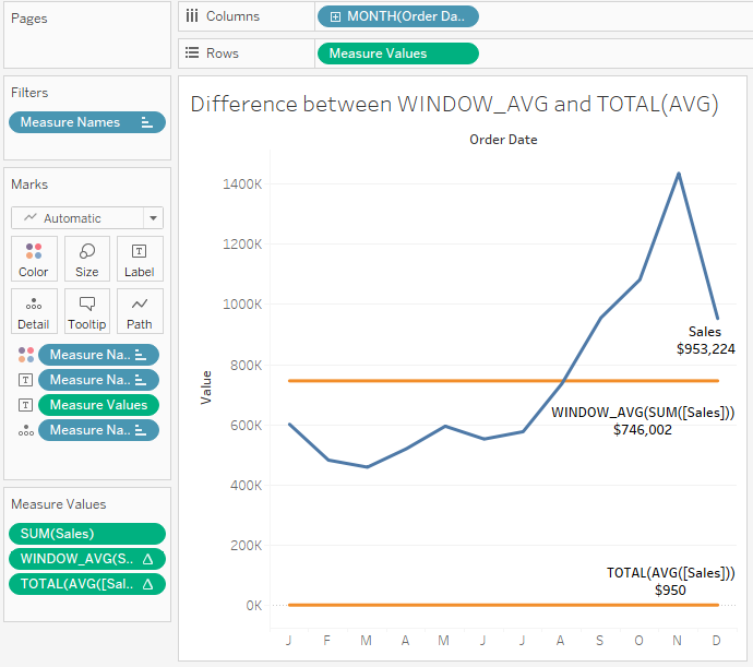
Figure 6.24: The difference between WINDOW_AVG() and TOTAL(AVG)

As you can see, WINDOW_AVG() gives you the average of the sums shown by the Sales line. TOTAL(AVG()) gives the overall total average of the underlying data set (in other words, the average sales line is $950).

In this section, we have looked at a number of table calculation functions. These will give you the building blocks to solve all kinds of practical problems and answer a great many questions. From ranking to year-over-year comparisons, you now have a foundation for success. Let’s now move on to some practical examples.

Practical examples

Having looked at some of the essential concepts of table calculations, let’s consider some practical examples. We’ll look at several examples, although the practical use of table calculations is nearly endless. You can do everything from running sums and analyzing year-over-year growth to viewing percentage differences between categories, and much more.

Year over year growth

Often, you may want to compare year over year values. How much has our customer base grown over the last year? How did sales in each quarter compare to sales in the same quarter last year? These types of questions can be answered using Year over Year Growth.

Tableau exposes Year over Year Growth as one option in the quick table calculations. Here, for example, is a view that demonstrates Sales by Quarter, along with the percentage difference in sales for a quarter compared with the previous year:

Figure 6.25: Year over year growth of Sales

The second Sum(Sales) field has had the Year over Year Growth quick table calculation applied (and the Mark type changed to bar). You’ll notice the >4 nulls indicator in the lower-right corner, alerting you to the fact that there are at least four null values (which makes sense as there is no 2016 with which to compare quarters in 2017).

If you filtered out 2017, the nulls that would appear in 2018 as table calculations can only operate on values present in the aggregated data in the cache. Any regular filters applied to the data are applied at the source and the excluded data never makes it to the cache.

As easy as it is to build a view like this example, take care because Tableau assumes each year in the view has the same number of quarters. For example, if the data for Q1 in 2017 was not present or filtered out, then the resulting view would not necessarily represent what you want. Consider the following, for example:

Figure 6.26: Year over year growth of Sales—but it doesn’t work with Q1 missing in the first year

The problem here is that Tableau is calculating the quick table calculation using the addressing of Year and Quarter and an At the Level of value of Year of Order Date. This works assuming all quarters are present. However, here, the first quarter in 2018 is matched with the first quarter present in 2017, which is really Q2. To solve this, you would need to edit the table calculation to only use Year for addressing. Quarter then becomes the partition and thus, comparisons are done for the correct quarter.

An additional issue arises for consideration: what if you don’t want to show 2017 in the view? Filtering it out will cause issues for 2018. In this case, we’ll look at table calculation filtering, or late filtering, later in this section. Another potential way to remove 2017 but keep access to its data values is to right-click the 2017 header in the view and select Hide.

Hide is a special command that simply keeps Tableau from rendering data, even when it is present in the cache. If you later decide you want to show 2017 after hiding it, you can use the menu for the YEAR(Order Date) field and select Show Hidden Data. Alternately, you can use the menu to select Analysis | Reveal Hidden Data.

You may also wish to hide the null indicator in the view. You can do this by right-clicking the indicator and selecting Hide Indicator. Clicking the indicator will reveal options to filter the data or display it as a default value (typically, 0).

Year over year growth (or any period over another) is a common analytical question that table calculations allow you to answer. Next, let’s consider another example of table calculations in practice.

Dynamic titles with totals

You’ve likely noticed the titles that are displayed for every view. There are also captions that are not shown unless you specifically turn them on (to do this, select Worksheet | Show Caption from the menu).

By default, the title displays the sheet name and captions are hidden, but you can show and modify them. At times, you might want to display totals that help your end users understand the broad context or immediately grasp the magnitude.

Here, for example, is a view that allows the user to select one or more regions and then see Sales per State in each Region:

Figure 6.27: Sales per State for two regions

It might be useful to show a changing number of states in the title as the user selects different regions. You might first think to use an aggregation on State, such as Count Distinct. However, if you try showing that in the title, you will always see the value 1. Why? Because the view level of detail is State and the distinct count of states per state is 1!

However, there are some options with table calculations that let you further aggregate aggregates. Or, you might think of determining the number of values in the table based on the size of the window. In fact, here are several possibilities:

• To get the total distinct count: TOTAL(COUNTD([State]))
• To get the sum within the window: WINDOW_SUM(SUM(1))
• To get the size of the window: SIZE()

You may recall that a window is defined as the boundaries determined by scope or partition. Whichever we choose, we want to define the window as the entire table. Either a relative computation of Table (down) or a fixed computation using all of the dimensions would accomplish this. Here is a view that illustrates a dynamic title and all three options in the caption:

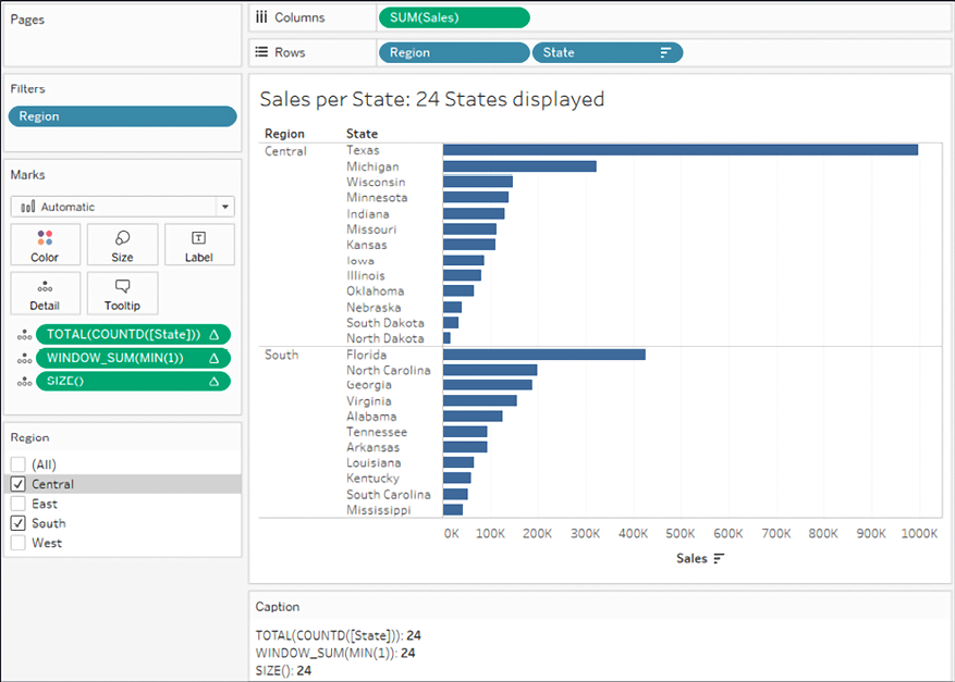
Figure 6.28: Various table calculations could be employed to achieve the total in the title

This example illustrated how you might use various table calculations to work at higher levels of detail, specifically counting all the states in the view. This technique will enable you to solve various analytical questions as you use Tableau. Let’s now turn our attention to another technique that helps solve quite a few problems.

Table calculation filtering (late filtering)

Let’s say you’ve built a view that allows you to see the percentage of total sales for each department. You have already used a quick table calculation on the Sales field to give you the percent of the total. You’ve also used Department as a filter. But this presents a problem.

Since table calculations are performed after the aggregate data is returned to the cache, the filter on Department has already been evaluated at the data source and the aggregate rows don’t include any departments excluded by the filter. Thus, the percent of the total will always add up to 100%; that is, it is the percentage of the filtered total, as shown in the following screenshot:

Figure 6.29: When Office Supplies is filtered out, the percentage table calculation adds up to 100% for the departments remaining in the view

What if you wanted to see the percentage of total sales for all departments, even if you want to exclude some from the display? One option is to use a table calculation as a filter.

You might create a calculated field called Department (table calc filter) with the code LOOKUP(ATTR([Department]), 0). The Lookup() function makes this a table calculation, while ATTR() treats Department as an aggregation. The second argument, 0, tells the lookup function not to look backward or forward. Thus, the calculation returns all values for Department, but as a table calculation result.

When you place that table calculation on the Filters shelf instead of the Department dimension, then the filter is not applied at the source. Instead, all the aggregate data is still stored in the cache and the table calculation filter merely hides it from the view. Other table calculations, such as Percent of Total, will still operate on all the data in the cache.

In this case, that allows Percent of Total to be calculated for all departments, even though the table calculation filter is hiding one or more, as shown in the following screenshot:

Figure 6.30: When a table calculation filter is used, all the aggregate data is available in the cache for the % of Total Sales to be calculated for all departments

You might have noticed the ATTR function used. Remember that table calculations require aggregate arguments. ATTR (which is short for attribute) is a special aggregation that returns the value of a field if there is only a single value of that field present for a given level of detail or a * if there is more than one value.

To understand this, experiment with a view having both Department and Category on rows. Using the drop-down menu on the active field in the view, change Category to Attribute. It will display as * because there is more than one category for each department. Then, undo and change Department to Attribute. This will display the department name because there is only one department per category.

In this example, we’ve seen how to effectively use table calculations as filters when we need other table calculations to operate on all the data in the cache.

Summary

We’ve covered a lot of concepts surrounding table calculations in this chapter. You now have a foundation for using the simplicity of quick table calculations and leveraging the power of advanced table calculations. We’ve looked at the concepts of scope and direction as they apply to table calculations that operate relative to the row and column layout of the view. We’ve also considered the related concepts of addressing and partitioning as they relate to table calculations that have computations fixed to certain dimensions.

The practical examples we’ve covered barely scratch the surface of what is possible, but should give you an idea of what can be achieved. The kinds of problems that can be solved and the diversity of questions that can be answered are almost limitless.

We’ll turn our attention to some lighter topics in the next couple of chapters, looking at formatting and design, but we’ll certainly see another table calculation or two before we’re finished!

Join our community on Discord

Join our community’s Discord space for discussions with the author and other readers: https://packt.link/ips2H